Estimating Network Link Characteristics using Packet-Pair Dispersion: A Discrete Time Queueing Theoretic View
Abstract
Packet-dispersion based measurement tools insert pairs of probe packets with a known separation into the network for transmission over a unicast path or a multicast tree. Samples of the separation between the probe pairs at the destination(s) are observed. Heuristic techniques are then used by these tools to estimate the path characteristics from the observations. In this paper we present a queueing theoretic setting for packet-dispersion based probing. Analogous to network tomography, we develop techniques to estimate the parameters of the arrival process to the individual links from the samples of the output separations, i.e., from the end-to-end measurements.
The links are modeled as independent discrete time queues with i.i.d. arrivals. We first obtain an algorithm to obtain the (joint) distribution of the separation between the probes at the destination(s) for a given distribution of the spacing at the input. The parameter estimates of the arrival process are obtained as the minimizer of a cost function between the empirical and calculated distributions. We also carry out extensive simulations and numerical experiments to study the performance of the estimation algorithm under the fairly ‘harsh’ conditions of non stationarity of the arrival process. We find that the estimations work fairly well for two queues in series and for multicast.
Keywords: Network tomography, packet-pair measurements, discrete time queues, packet-pair tomography, multicast queues.
1 Introduction and Background
Network tomography is the estimation of detailed statistics of performance parameters from aggregate or end-to-end measurements of some measurable quantity. The term was first coined in [1], where the problem of estimating flow volumes from link volumes was analyzed. This is also called the traffic matrix estimation problem and has been extensively studied in the transportation literature, for which, an excellent survey is available in [2]. The traffic estimation problem is now being addressed by the networking community ([3, 4, 5, 6, 7]. Another network tomography problem is that of estimating link delay statistics from the samples of end-to-end delays experienced by multicast packets [8, 9]. Much of the work in this area has been in estimating the link or segment delay distributions from the end-to-end measurements. See [10] for a fairly comprehensive survey of both delay and traffic estimation tomography problems and solutions related to networking.
The bandwidth on a network path has also been of significant interest and a number of tools have been developed for its estimation. Two kinds of bandwidth related metrics are often estimated. The bottleneck bandwidth is the maximum transfer rate that could be achieved over a path and is essentially the minimum of the transmission rates on the links in the path. The available bandwidth is the portion of the bottleneck bandwidth not used by competing traffic and depends on the traffic load at the inputs to the links.
Many tools have been developed to measure the bottleneck and available bandwidths. To the best of our knowledge, all these tools are based on either ‘packet-pair’ or ‘packet-dispersion’ techniques. The packet-pair technique was first described in [11] to measure the bottleneck bandwidth on a path where the links are rate-servers. In this technique two back-to-back packets of equal length are transmitted by the source. It can be shown that the ratio of the probe packet length to the separation between them at the receiver is the service rate for the packet at the bottleneck link on the path. This idea has been used to develop many tools, e.g., pathchar [12] and clink [13], that measure the bottleneck capacity of a network path. Inspired by the packet-pair technique, the packet-dispersion, also called packet-spacing, technique has been developed to measure the available bandwidth of an Internet path [14, 15, 16, 17, 18]. In this technique, a source transmits a number of probe packets with a predetermined separation, say The samples of the separation at the receiver, say are then used to estimate the available bandwidth on the path. pathload [14] and pathChirp [15] are some examples of tools that use the packet-spacing technique to measure the available bandwidth. See [16] for an excellent survey of the different packet-spacing techniques used in the measurement tools and [17] for an experimental comparison of the tools. A non cooperative version that does not require a measurement-enabled receiver is described in [18].
Packet-pair and packet-dispersion techniques have an important advantage in that they do not require the sender and the receiver to be synchronized in time. This makes them important in practice. However, the tools that employ these techniques are based on informal arguments. There have been excellent statistical studies based on experiments on packet-pair techniques (e.g., [19, 20]). Recently, there have been a few theoretical models developed for packet dispersion based bandwidth probing techniques [21, 22, 23, 24, 25, 26, 27]. In [21, 22] it is shown that the output dispersion of probe pair samples the sum of three correlated random processes that are derived from the traffic arrival process. The asymptotics of these and the probing process are also analysed. The measurement methods of some bandwidth estimation tools are then related to the analytical models developed. These results are then extended to multihop paths in [23]. In [24], the network is assumed to be a time-invariant, min-plus system that has an unknown service curve. This service curve estimation method is developed for different probing techniques.
While the above works provide interesting theoretical insights into the probing process, our work is more closely related to that of [27, 25, 26]. In [27], a probe train is assumed and the actual delay of each of the probe packets is assumed to be known at the output of the path. The delay sequence is assumed to form a Markov chain whose transition probability matrix is estimated. An inversion is defined to estimate the characteristics of the arrival process from the transition probabilities of the delay Markov chain. In [25], the bottleneck link is modeled as an M/D/1 queue, and the expected dispersion is calculated using the transient analysis. The method of moments is then used to estimate the arrival rate. A similar method is followed in [26] where the more general M/G/1 queue is considered and Takacs’ integro-differential equation is used to obtain the distribution of the dispersion.
In this paper we develop techniques to estimate the parameters of the arrival process distribution on the individual links on a path or a multicast tree from packet-dispersion samples in a queuing theoretic setting. Packet-pair probes with predetermined separation between them are injected at a source. These probe packets traverse discrete-time queues with i.i.d. packet arrivals on a path or in a multicast tree. Samples of the separation between the probe packets at the output nodes of the path or the multicast tree are used to estimate the parameters of the arrival process distribution at the individual links. The approach is as follows. First, for a single queue and for a given separation between the probes at the input, we derive the conditional distribution of the separation between the probes at the output of the queue in terms of the distribution of the arrival process to the discrete time queue. The key intermediate result here is the joint distribution of the number arrivals to the queue and the number of departures from the queue between the slots in which the probes are injected. Then the output separation is obtained for any given distribution of the input separation. Since the input separation distribution is known, (we assume it to be fixed) this is applied recursively on the path to obtain the separation distribution at the outputs. The parameter estimator is the minimizer of a suitable distance function between the empirical and the theoretical distributions of the output separations.
We first develop our results by assuming that the probe packets are served after all the packets that arrive in their slot, i.e., the probe packets have the least priority among the packets that arrive in their slot. Extension to the case of the probe packet having the same priority (or any arbitrary fixed priority) as the other packets that arrive in the slot will be along the same lines and is also presented. We present numerical results only for the first case, i.e., when the probes have lowest priority.
Our modeling assumption is similar to that of [27] in that we also consider discrete time queues. While [27] considers the delay process of the probe sequence, we consider the dispersion of the packet pair. The inversion methods are also different. While we consider a general i.i.d. arrival process for the discrete time queeu, [25] considers an M/D/1 queue and obtains approximations, [26] considers an M/G/1 queue.
The rest of the paper is organized as follows. In the next section, we describe the problem setting and the notation that we will be using in the paper. In Section 3 we consider a single pair of probes that are injected into a stationary discrete-time queue and develop an algorithm for computing the distribution of the separation between a pair of probes at the output of a single queue when the distribution of the separation at the input of the queue and also the arrival process distribution are known. In Section 4, we consider sending the probes over a multi-link path and over a multicast tree and obtain the distribution of the output separation(s) between the probes at their outputs. In Section 5 we describe the method to estimate the parameters of the arrival process at the queues. The numerical evaluation of the estimates for the case of Poisson arrivals are discussed in detail in Section 6. In Section 7, we describe a generalization and an extension to the basic theory developed in Section 3. In particular, we outline the method for computing the output separation distribution when the probes have equal priority with the packets arriving in the same slot. We conclude with a discussion in Section 8 where we explore connections with an earlier theoretical study of packet-dispersion techniques. We also contrast our results with delay-tomography results.
2 Notation and Preliminaries

We first describe the notation used in this paper. For pedagogical purposes, we consider a packet queuing system. In this section we will consider a single-server queue with infinite buffers and FCFS service discipline. The service time of each packet is equal to the slot length. The convention will be as follows. Packet arrivals to the queue in slot will occur at the beginning of the slot and the departures will occur at the end of the slot. Thus arrivals in a slot will be available for departure in the slot. We observe the queue at the beginning of a slot, just after the arrival instant. Let denote the number of packets that arrive in slot the number of departures in slot and the number of packets in the queue when the queue is observed at the beginning of the slot. This convention is shown in Figure 1. Of course, can only be or Further, for will denote the cumulative arrivals in the interval and will denote the cumulative departures in the interval In particular, and Note that is a function of and will denote the number of departures in slots that the same arrival sequence would cause with Observe that this makes independent of the distribution of and a function of only The work-conserving, FCFS service discipline will be applied at the granularity of the batch of packets that arrive in a slot and the packets in a batch will be queued in a random order. The queue evolution equation as per the above convention will be
| (1) |
In the rest of this paper we assume that the arrival sequence is i.i.d. and let Recall that if then the queue length process is stationary and the moment generating function of the stationary queue length distribution is given by
where is the moment generating function of In fact can be obtained using the following recursion.
3 Passage of a Probe Pair through a Discrete Time Queue
In this section we consider injecting a single probe pair into a stationary queue and derive the distribution of the output separation, as a function of the input separation, and the parameters of the packet arrival process For a given distribution of the input separation, the distribution of is obtained as
| (3) |
Let us consider a queue in steady state. Consider two probe packets, denoted by and inserted into the discrete time queue in slots and respectively. Since we are considering stationary queues, without loss of generality, we can relabel the slots in this manner. These probe packets are enqueued along with the other packets that arrive in their respective slots and are available for transmission in the same slot in which they arrive. In this section, we assume that the probe packets have the least priority among the packets that arrive in their slot.
Let and denote the departure slots for the first and the second probe respectively. Let denote the dispersion of the probe packets at the output of the queue. Clearly,
| (4) |
is the packet-dispersion. In the above, does not include probe packet and is the number of packets in the queue at the beginning of slot not including Also, does not include while includes the possible departure of Note that since the queue has packets (including ) in slot Observe that the separation between the probes at the output of the queue, is affected by the arrivals and departures between the arrivals of and , i.e., by and Thus, to obtain the conditional distribution of the output separation, given the input separation, we need to obtain the joint distribution of the number of arrivals and departures between the two probe pairs. Computation of this joint distribution is the key to the computation of the distribution of the output separation.
From Eqn. 4, for a given , say the distribution of the output separation can be expressed as
| (5) |
for . Since we are assuming that we are probing a stationary queue, the first probe packet will see the queue in steady state. We can then obtain the joint distribution of and as
| (6) |
We can see that and are independent of each other, but is dependent on both and on the finite sequence We make the reasonable assumption that the distribution of is known since it can be derived from the distribution of , albeit as a function of its parameters. Hence, to obtain the distribution of we first need to obtain the joint distribution of and conditioned on i.e., the joint distribution of and This is derived in the following subsection.
3.1 Joint Distribution of and
In this section we first obtain a recursion on for the joint distribution of and and then, for arbitrary express the joint distribution of and in terms of the joint distribution of and We thus begin with the case of From our notation, this means that when the first probe packet is injected into the queue in slot it is the only packet in the queue. Since there is the probe packet to be transmitted in slot Thus we have the following base equations for the joint distribution.
Now, for arbitrary we can write the following one-step recursion which also spells out the kind of recursion we seek.
| (8) |
For ease of exposition, define
We now consider three cases.
- 1.
If or then This is because, for there to be departures in slots the number of departures in slots , denoted by should be either or
- 2.
If , then there has to be a departure in slot Since this is possible if, and only if, because only then will the total number of arrivals in slots including be greater than or equal to Hence, for and for is a sure event and requires that packets have to arrive in slot giving us
- 3.
For there should be no departure in slot Since has departed in slot Hence the total number of departures in slots i.e., should be the same as Therefore, for Thus for only will yield a non zero when the number of arrivals in slot is i.e., for and we have
Combining the above three cases, we can rewrite the recursion in Eqn. 8 for the joint distribution of and as
| (9) |
We obtain the joint distribution and by a suitable transformation of the joint distribution of and derived above. To obtain we consider the following cases. Clearly, this probability is zero if (the number of departures is greater than the number of slots) and for
- 1.
The number of departures in slots is less than the number of slots, i.e., We consider two sub cases.
- (a)
Clearly, is not possible because in that case, the number of departures including the probe packet would have been at least Therefore, for
- (b)
For the event
is the same as the event
and so
Thus, for we get
- (a)
- 2.
If , then there is a departure in every slot in We once again consider two sub cases.
- (a)
If then the event
is the same as the union of the disjoint events
for Hence, for this case, we can write
- (b)
If the queue starts with packets, then there will be a departure in every slot and is a sure event and so for this case .
- (a)
Summarizing the above, we have the following transformation.
| (10) |
Once the joint distribution of and is found using the joint distribution of and the joint distribution of and can be found from Eqn. 6.
The infinite summations in Eqns. 6 and 3 will need to be truncated in practice. Let and respectively denote the truncation limits. Also, in Eqn. 5 we need to limit the range of the output separation for which we will compute the probabilities. Let be this limit. The algorithm for computing the distribution of the output separation is summarized in Fig. 2. The recursion in step 3b of Fig. 2 is computationally the most intensive part of the algorithm. It can be shown that this step requires
additions and multiplications.
- 1.
Input: Arrival distribution Input separation distribution - 2.
Obtain using the following equations.
- 3.
Obtain the joint distribution of for each using the following equations.
- (a)
Base Equations
- (b)
Recursions
- (c)
Transformations
- (a)
- 4.
Obtain the joint distribution of by using the following equations.
- 5.
Obtain the output separation distribution for a given input separation, say
- 6.
Obtain the distribution of the output separation for a given input separation distribution.
4 Passage of a Probe Pair through a Network of Independent Queues
We now characterize the output separation between the probes as they pass through multiple queues. Since we are able to express the distribution of the output separation of the probe pair in terms of the distributions of the input separation and the arrival process distribution, we can obtain the distribution of the output separation at the output of a path of independent queues fairly easily.

We first consider the case when the probe pair passes through a path consisting of independent queues as shown in Figure 3. The probe packets leaving queue are placed in queue after an arbitrary but fixed delay. Since the delays are fixed, the separation between the probe pairs at the input to queue is the same as that at the output of queue . (Generalization to variable delay is presented in Section 7.) Let be the separation at the input to queue 1 and the separation between the probe pairs at the output of queue with
For let denote the i.i.d. arrival sequence into queue the distribution of and the stationary distribution of the queue occupancy at the beginning of a slot. Probe packets and are injected into queue 1 in slots and respectively with a known distribution of The distribution of is obtained from the recursive relation
| (11) |
The distribution of can be obtained by repeated use of the algorithm in the previous section from the distribution of . Notice that, if then has the same distribution as
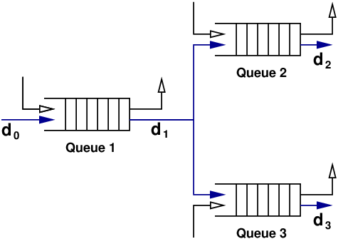
The second case that is of interest is when the probe pairs traverse a multicast tree of independent queues. Figure 4 shows an example of a three-node tree. Here copies of the probe packet are made at the output of Queue 1 and the copies are simultaneously placed in queues 2 and 3 after arbitrary but fixed delays on each of the links. As with the case of a path, since the delays are fixed, the separation between the probe pairs at the input to queues 2 and 3 is the same as that at the output of queue 1. We are interested in the joint distribution of the separation at the output of both queues 2 and 3, and respectively. This joint distribution is given by
| (12) |
The last equality follows because conditional on and are independent. The individual conditional probabilities can be obtained as before.
The above ideas can be extended to compute the joint distribution of the separation at the leaves of an arbitrary tree rooted at the node which introduces the probe pairs into the network.
5 Estimating the Arrival Process Parameters
The algorithm developed for computing the distribution of the output separation between the probes can, in principle, be used to estimate the traffic parameters in the network provided the parameters are identifiable from the distribution. However, often the parameters may not be identifiable from the distribution, i.e., the same distribution may be resulted from two different sets of traffic parameters. For instanct, consider a series of two queues with independent Poisson traffic with means and . The output separation has the same distribution for and . We performed some simulation experiments to judge the viability of using this distribution for traffic parameter estimation. However, these simulations use ideal settings like independent Poisson traffic arrivals to different queues which are usually not strictly satisfied by practical networks, and as a result, should be taken only as proof of concept. They do not guarantee that the method will work in practical networks.
Consider a rooted tree of independent queues. Probe pairs are introduced into this network at the root of the tree with unit separation. While the theory allows for an arbitrary but known distribution of the input separation, we choose a fixed input separation of one slot. This minimizes the computational requirements.
The separation between the probe pairs at the output of the leaves is observed. We assume that there is no loss of probe pairs in the network. We also assume that the link delays, i.e., the delay between the output of a queue and the input to the next queue on a path is arbitrary but fixed.
For let be the arrival sequence of packets into queue For queue is an i.i.d. sequence and further, the sequences for the different queues are independent. Let be the vector of parameters of the distribution of and let us define Our goal is to estimate by observing only the separation of the probes at the output of the leaves of the paths. Let denote these leaf nodes and the separation of the probe pairs at the output of these queues.
We send a sequence of probe pairs and corresponding to every probe pair we obtain an observation of the vector From these observations we can obtain the empirical distribution of denoted by . We probe with a very low rate, i.e., the interval between the probe pairs is made very large so that the probing load is negligible. This allows us to assume that the stationary distribution of the occupancy of queue is governed only by the distribution of and is a function of only Further, we assume that the first packet of every probe pair, packet , ‘sees’ each of the queues in steady state. This allows us to express the distribution of as a function of only We then use the results of the previous sections to compute the analytical distribution for a given value of Let denote a suitably defined distance between and The estimate of the parameter vector can be obtained as
i.e., is obtained as the minimizer of the distance between the empirical and the analytical distributions of the separation vector.
A well known measure of the distance between two distributions is the Kullback-Leibler (KL) distance. The KL distance between the empirical and the analytical distributions for a given is defined as
It can be shown that the minimizer of is the maximum-likelihood estimate of Alternatively, we could use the squared Euclidean distance, as the measure of the distance between the two distributions. The squared Euclidean distance between the empirical and the analytical distributions for a given is given by
A simplistic way to obtain is as follows. The analytical distribution is computed and stored for all the values of the parameter vector over a suitably discretized grid on the feasible range of . We obtain the empirical distribution from a sufficiently large number of probes. The minimizer of is then obtained by an exhaustive search over the grid. To find a reasonably accurate estimate, the exhaustive search will require a very fine grid and consequently a large number of distribution calculations. Rather than an exhaustive search, we can also use an optimization method to reach the minimum of
As we had mentioned earlier, for the case of one queue, if we fix then will have the same distribution as and estimating the parameters of is straightforward. We will not pursue that any more. The case of a two-queue path has interesting numerical properties and we explore them in detail in the next section. This will give us an insight into the difficulties of probing paths that have multiple bottlenecks. We expand upon this in Section 7. We will also see that the estimation quality when probing a multicast tree is significantly better.
6 Numerical Results
In this section we present some numerical results obtained as follows. Different paths and multicast trees of independent discrete-time queues are simulated. The probe packets are injected into the system at very low probing rate. The passage of the probes through the different queues are simulated and the output separation obtained for each probe. We do not simulate lost probes although it is easy to see that they do not affect the algorithm. Although our results are applicable for all distributions of the arrival process, we report our results for the case when the packet arrivals form an i.i.d. Poisson sequence. Since Poisson is a one-parameter distribution, it is easier to discuss the issues in the estimation of
We first consider a two-queue path. Let and be the arrival rates of packets to queues 1 and 2 respectively. Probe pairs are generated according to a Poisson process. We obtain the empirical distribution from slots of simulation time. Table 1 shows the estimates that minimize the squared Euclidean distance and KL distance between the empirical distribution and the calculated distribution for different true values of and and for two probing rates. Notice that both the distance measures give comparable precision in almost all cases. Since the squared Euclidean distance is computationally simpler than the KL distance, the rest of the numerical results are based on the squared Euclidean distance.
| True | inter | Estimates in 3 different executions | |||||
|---|---|---|---|---|---|---|---|
| values | probe | Euclidean cost based | KL distance based | ||||
| mean | |||||||
| (0.9, 0.8) | 1000 | ||||||
| ” | 200 | ||||||
| (0.5, 0.6) | 1000 | ||||||
| ” | 200 | ||||||
| (0.7, 0.4) | 1000 | ||||||
| ” | 200 | ||||||
| (0.2, 0.3) | 1000 | ||||||
| ” | 200 | ||||||
The exhaustive search method has the drawback that it is primarily a one time estimation and not an adaptive one. An alternative is to reach the optimum value by a suitable optimization algorithm, for example, a steepest descent algorithm. This may not however give the best estimate if the distance function has a local minima. We performed an extensive numerical investigation of the nature of the cost function for the two-queue case. However, the cost function was seen to be non-convex. The level sets of the Euclidian cost function as shown in Fig. 6 are clearly not convex. This may present some problem in convergence of an optimization technique. However, the limited numerical simulations performed by us gave reasonably good performance under ideal setup.


Fig. 5 shows the plot of a typical Euclidean cost function for an empirical distribution obtained from simulation with . The minima is at . However, notice that the function shows a distinct valley along a line with an extremely low slope along it. The existence of the valley is more clear from the contour plot of the cost function shown in Fig. 6. The steepest descent method will result in a very slow convergence due to zig-zagging along the valley.
Our main simulation involves an iterative stochastic gradient based online estimation. We divide the probe sequence into equal sized blocks and compute the ‘instantaneous’ empirical distribution of for every block. In our simulations we have used a block size of 500. Let be the instantaneous empirical distribution obtained from the -the block of probes. The overall empirical distribution after the -th iteration, is updated using the exponential update rule
| (13) |
Here is a constant between and . We used in all our simulations. For each , we then update our estimate of based on the current empirical distribution . We use the steepest descent algorithm for one iteration for each and update the estimate of as
where denotes the length of a vector and is the step size. We used an adaptive step size so that whenever a particular step increases the distance, the step size is decreased and whenever the gradient is more than a threshold, the step size is increased. The increase and decrease of the step size is not done if it is respectively above or below some thresholds. If the arrival process is non stationary, this scheme allows us to track slowly varying Our simulations will study the effectiveness of such tracking.


We first consider the two-queue path. and are varied linearly with time and a step change is also simultaneously introduced. Fig. 7 plots the true values of and and the estimates as functions of time. For the estimation, the initial estimates are taken as From these plots we see that the steepest descent algorithm converges and tracks the true values reasonably well even when there is step change. It is instructive to study the evolution of the estimate. Fig. 8 shows the evolution of the estimate pair A close look at the figure reveals that initially as well as when the parameters change suddenly, the estimates go to the nearest point on the new valley and then zig-zags along the valley towards the true values.

We next consider the three-queue multicast tree of Fig. 4. As with the two-queue case, the true values of are varied linearly and also a step change is introduced. In Fig. 9 we plot , and as functions of time along with the true values. Observe that these estimates are far superior to those for the two-queue path. This is because here we have the empirical joint distribution of the output separations at two leaf nodes of the network and this gives much more information about the arrivals to the queues.
The slow convergence of the adaptive estimation due to the valley in the Euclidean cost function that we saw for the two-queue path is expected to be even more pronounced for a three-queue path. In fact, in our simulations, the estimates did not converge to the true values even after slots of simulation time. We conjecture that there will be a valley along a two dimensional manifold.

We have seen that in a multicast network, having multiple outputs through different paths helps improve the quality of the estimation. However two or more queues in series makes for slow convergence of the estimates. To investigate the interplay of these two we carried out the estimation for a four-queue multicast tree shown in Fig. 10. The plots of the estimates and the true values of the arrival means are shown in Fig. 11. As expected, we observed faster convergence for this network. However, the queues 2 and 4 are in series in this network. The estimates of and can be seen to be worse than the estimates for the two-queue path. This is possibly because of the error in the estimate of (this misleads the estimation of and with an incorrect distribution of the probe separation at the input of queue 2) and also because the probe pairs entering queue 2 are not separated by a fixed one slot. Hence, the convergence of the estimates of and is not as fast as that of and .

In the adaptive estimation, we need to consider two performance criteria. If the arrivals are stationary, we need to minimize the error in the estimate. However, if the arrivals are non-stationary, we would like the estimates to track the true values closely. Achieving these objectives is governed by the choices of the various parameters of the estimation algorithm. In the rest of this section we will discuss the role of these parameters. The performance of the estimation was seen to be quite sensitive to the selection of the parameters, and quite a bit of tuning was necessary to get the performance shown in the figures.
Choice of block length and : The parameter (in Eqn. 13) and the number of probe pairs in a block dictate how fast the empirical distribution tracks the true distribution of the output separations. However, there is a trade-off between tracking the true distribution for non-stationary arrivals and the variance of the empirical distribution under stationary arrivals. Increasing or decreasing the block size enables the empirical distribution to track the actual distribution faster but increases the variance of the empirical distribution under stationary arrivals. This reflects in tracking the true value faster but in the components of having larger variance under stationary arrivals.
The step size also plays a role in the convergence rate and the tracking ability of the estimation. A larger enables faster tracking but results in larger variance of the estimates under stationary arrivals.
How well to track the minima of : In our simulations, we have used one iteration of steepest descent for each . Alternatively we could use an exhaustive search to obtain the minima of As a second alternative, we may execute many iterations of steepest descent for each . This may involve a fixed number of iterations or termination based on a specified condition. A larger number of iterations for each will enable to be nearer the minima of the current cost function Hence, a larger number of iterations for each will result in the estimate tracking the minima of more closely. Although this results in better tracking, it makes the estimate more tuned to the current empirical distribution and as a result more sensitive to the variation of the current empirical distribution under stationary arrivals.
Alternative Optimization Methods: The valley in the cost function makes the convergence of steepest descent algorithm very slow due to the typical zig-zag path followed by this algorithm. Other optimization algorithms like conjugate gradient or Newton’s algorithm may also be tried to overcome the problem.
Method of Moments Based Estimation: A common method in parameter estimation is the method of moments. A similar approach can be considered here. We can compute a few moments of the calculated and the empirical distribution and try to match them by varying the parameters. In the absence of closed form expressions for the moments, we may again need to estimate by minimizing a suitable cost function between the calculated moments and the moments from the empirical distributions. However, since we do not have a way of calculating the moments directly without calculating the distributions first, this method presents little attraction, especially since we can expect to lose some information in working only with some moments instead of the distributions themselves. Indeed, the results obtained by using the squared Euclidean distance between the vectors of the first ten moments of the calculated and the empirical distributions gave no promising results. It is also to be noted that computation of higher order moments is computationally intensive and needs numerical caution in dealing with large numbers.
Probing rate: Finally, we remark on the probing rate. A higher probing rate gives us more samples and hence a quicker convergence for stationary arrivals and a better ability to track fast changing arrival processes. However, the probing process makes the aggregate arrival process, including the probe packets, non Poisson and disturbs the estimate because the calculated distribution will not be correct. Further, the samples may not be independent if the probes are closely spaced. To minimize the effect, the mean probe arrivals should be small. In our simulations, the times at which probes are inserted were generated according to a Poisson process of rate
7 An Extension and a Generalization
In this section we consider an extension and a generalization to the algorithms presented in Sections 3 and 4. First, we relax the assumption that the probe packet has the least priority within its batch. We will see that this essentially involves extension of the joint distribution of and of Section 3.1 to include packets that arrive in the same slot as the probes but may be queued after the probe packet. We then present a generalization in which we allow the transfer delays in the network to be random rather than fixed but arbitrary.
7.1 Generalization to Equal Priority for the probes
In our discussions earlier, we assumed that the probe packets have the lowest priority among the packets that arrive in the slot. We now consider the case when all the packets that arrive in a slot have the same priority and the position of the probe packets within the batch may have a distribution.

For convenience, we redefine the notation and let be the number of packets in the queue at the beginning of slot but before the arrival of the packets in slot . This new notation is shown in Figure 12. Under this notation the queue evolution described by Eqn. 1 changes to
| (14) |
Note that according to this definition the stationary distribution of would be different from that given in Eqn. . The probability generating function for the stationary distribution would be
and the recursion for the probabilities will be
For a probe packet arriving into the queue in slot define (resp. ) to be the number of packets from those that arrived in slot that are queued before (resp. after) the probe packet. Thus Also, for probe packets arriving in slots and define,
As before, we assume that the probe packets and enter the queue in slots and respectively. They depart in slots and . Along the lines of Eqn. 4 we obtain the output separation of the probe packets as follows.
| (15) | |||||
For any to obtain the distribution of the output separation, we thus need to know the joint distribution of and
The distribution of and is derived from the distribution of as
Following the procedure in obtaining the recursion in Section 4 we begin by defining to be the number of departures in slots when and
As before, we begin by assuming and compute the joint distribution of and The base equation will be
Here is an empty summation and we define it to be 0. We first obtain the recursion for the joint distribution of and and then the joint distribution of and Following the arguments of Section 3, we obtain the following recursions.
| (17) | |||
| (18) |
where is the Kronecker delta function. If and then, following the arguments in the development of Eqn. 10, the joint distribution of and would be obtained in exactly the same manner as Eqn. 10, except that would be replaced by . Thus we will have
| (19) |
Of the packets that arrive in slot , if are queued after then we need that many fewer arrivals in Hence, we have
| (20) |
Finally, we can uncondition on and as
| (21) |
The output separation of the probes can now be obtained following the same method as in Section 3.
7.2 Random Delays on the Links
In deriving the distribution of the output separation, in Eqns. 11 and 12, we assumed that the transfer delays from the output of a queue to the input of the next queue on the path is arbitrary but fixed. We can relax this requirement as follows.
Consider the series of queues of Figure 3 first. In going from the output of queue to the input of queue , let be delayed by slots and by slots. Let be the probe separation at the output of queue The probe separation at the input to queue is It is reasonable to assume that the order of the probes is maintained in the transfer from to . Hence and cannot be independent. If the conditional distribution of given is known then Eqn. 11 can be generalized as

Along similar lines, we can generalize for random transfer delays on the multicast tree. The schematic is shown in Fig. 13. Eqn. 12 can be generalized as
There are many uses for this generalization. If the transmission rates on the links are different, then the separation is compressed or expanded depending on whether the downstream link has a higher or lower data rate respectively. The conditional distribution of the separation can be obtained by knowing the two transmission rates.
A second use is in tomography of paths with many links with one or two of them being ‘bottleneck links.’ Consider a -queue path. Let links and be the bottleneck links. The delays from the source to the input of link , from the output of to input of and from the output of to the destination can have simple models. For example, let and with link being lightly loaded. We can assume that over link 2, each of the probes and will see at most one cross traffic packet independently. Let be the probability of this event. Then we can see that, if the input separation is greater than 1, the separation increases by 1 if only is sees a cross traffic packet, while it shrinks by 1 if only sees such a packet. If the input separation is 1, then the output separation will also be 1 if neither does not see a cross traffic packet. We can then use
Here link 2 is playing the role of the random delay element.
8 Discussion and Conclusion
We conclude with a discussion on the connection with some earlier results on the analysis of packet-dispersion based probing and also on network delay tomography.
We first explore the connection of this work with that in [21, 22]. A theoretical analysis of packet pair probing of a single bottleneck path is carried out in [21]. A continuous time model is used and the key result is Theorem 2. This theorem states that for a probe pair inserted into the queue at time with input separation and probe packet length the output separation is given by
| (22) |
where
- •
is the capacity of the bottleneck link,
- •
is the work (sum of the service times of the packets) that enters the queue in and
- •
is the unused capacity of the server in the interval
Thus the output separation is a sample of a linear combination of three interdependent random processes. This theorem essentially implies that obtaining the joint law of these processes is the key to the use of packet pair probing.
We can interpret Eqn. 22 for the discrete time queues that we consider as follows. Note that The first term is the number of packets entering the queue between the enqueuing of the two probe packets and the third term is the number of idle slots between the enqueuing of the two probe packets. Thus we can rewrite Eqn. 22 as follows.
The last equality is true because the number of departures in slots can never be greater than This is nothing but Eqn. 4!
Eqn. 22 essentially says that the output separation of a packet pair is a function of the work entering the queue between the probe arrivals and the amount of work done in this interval. These two quantities are dependent and one needs their joint distribution for finding the distribution of The key difficulty in developing the analytical model for packet pair probing is to obtain this joint distribution, and we believe, that is a key contribution of this paper.
It is interesting to contrast our problem setting with delay tomography of, for example, [8, 9], since both estimate how the individual links will affect the traffic flowing, albeit, in different forms. An important assumption in the development of network-delay tomography is that the end-to-end delays of the individual packets can be measured. This requires that the sources and the destinations be suitably time synchronized. This is clearly not an easy task. In fact, the packet-pair techniques were developed to avoid this problem. Furthermore, much of the delay-tomography results were developed assuming that the probes are multicast packets. This means that when there are links in series, the estimation is for the delay across the series and not on the individual links.
Finally, we remark that the primary objective in this paper is to develop an analytical framework for ‘capacity tomogrpahy’ and not develop a practical tool.
References
- [1] Y. Vardi, “Network tomography: Estimating source-destination traffic intensities from link data,” Journal of the American Statistical Association, vol. 91, pp. 365–377, March 1996.
- [2] T. Abramsson, “Estimation of origin-destinaion matrices using traffic counts—a literature survey,” Tech. Rep. IR-98-021, International Insitute of Applied Systems Analysis, May 1998.
- [3] Y. Zhang, M. Roughan, C. Lund, and D. Donoho, “An information-theoretic approach to traffic matrix estimation,” in Proceedings of ACM SIGCOMM, Kalsruhe, Germany, August 25–29 2003.
- [4] Y. Zhang, M. Roughan, N. Duffield, and A. Greenberg, “Fast accurate computation of large-scale ip traffic matrices from link loads,” in Proceedings of ACM SIGMETRICS, 2003.
- [5] A. Medina, N. Taft, K. Salamatian, S. Bhattacharyya, and C. Diot, “Traffic matrices estimation: Existing techniques and new directions,” in Proceedings of ACM SIGCOMM, 2003.
- [6] A. Lakhina, K. Papagiannaki, M. Crovella, C. Diot, E. D. Kolaczyk, and N. Taft, “Structural analysis of network traffic flows,” in Proceedings of ACM SIGMETRICS, 2004.
- [7] K. Papagiannaki, N. Taft, and A. Lakhina, “A distributed approach to measure ip traffic matrices,” in Internet Measurement Conference (IMC) ’04, Taormina, Sicily, Italy., October 25–27 2004.
- [8] M. J. Coates and R. Nowak, “Network tomography for internal delay estimation,” in Proceedings of IEEE International Conference on Acoustics, Speech, and Signal Processing, 2001.
- [9] Y. Tsang, M. J. Coates, and R. Nowak, “Passive network tomography using em algorithms,” in Proceedings of IEEE International Conference on Acoustics, Speech, and Signal Processing, May 2001.
- [10] R. Castro, M. J. Coates, G. Liang, R. Nowak, and B. Yu, “Internet tomography: Recent developments,” Statistical Science, vol. 19, no. 3, pp. 499–517, 2004.
- [11] S. Keshav, “A control-theoretic approach to flow control,” ACM SIGCOMM Computer Communication Review, vol. 21, no. 4, pp. 3–15, September 1991.
- [12] V. Jacobson, “Pathchar: A tool to infer characteristics of internet paths,” April 1997.
- [13] A. B. Downey, “Using pathchar to estimate internet link characteristics,” in Proceedings of ACM SIGCOMM, September 1999, pp. 222–223.
- [14] M. Jain and C. Dovrolis, “End-to-end available bandwidth: Measurement methodology, dynamics, and relation with tcp throughput,” in Proceedings of ACM SIGCOMM, August 2002, pp. 295–308.
- [15] V. J. Ribeiro, R. H. Riedi, R. G. Baraniuk, J. Navratil, and L. Cottrell, “pathChirp: Efficient available bandwidth estimation for network paths,” in Proceedings of Passive and Active Measurement Workshop, 2003.
- [16] R. Prasad, C. Dovrolis, M. Murray, and k. claffy, “Bandwidth estimation: metrics, measurement techniques, and tools,,” IEEE Network, vol. 17, no. 6, pp. 27–35, November–December 2003.
- [17] J. Strauss, D. Katabi, and F. Kaashoek, “A measurement study of available bandwidth estimation tools,” in Proceedings of the 3rd ACM SIGCOMM conference on Internet measurement, Miami Beach, FL, USA, 2003, pp. 39–44.
- [18] S. Chakraborty, B. Walia, and D. Manjunath, “Non cooperative path characterisation using packet spacing techniques,” in Proceedings of IEEE Conference on High Performance Switching and Routing (HPSR), Hong Kong PRChina, May 2005.
- [19] C. Dovrolis, P. Ramanathan, and D. Moore, “What do packet dispersion techniques measure?,” in Proceedings of the IEEE INFOCOM, Anchorage, AK, USA, April 2001, pp. 905–914.
- [20] A. Pasztor, Accurate Active Measurement in the Internet and its Application, Ph.D. thesis, Department of Electrical and Electronic Engineering, The University of Melbourne, February 2003.
- [21] X. Liu, K. Ravindran, and D. Loguinov, “What signals do packet-pair dispersions carry?,” in Proceedings of the IEEE INFOCOM, March 2005, pp. 281–292.
- [22] X. Liu, K. Ravindran, and D. Loguinov, “A queuing-theoretic foundation of available bandwidth estimation: Single-hop analysis,” IEEE/ACM Transactions on Networking, vol. 15, no. 4, pp. 918–931, August 2007.
- [23] X. Liu, K. Ravindran, and D. Loguinov, “A stochastic foundation of available bandwidth estimation: Multi-hop analysis,” IEEE/ACM Transactions on Networking, vol. 16, no. 1, pp. 130–143, February 2008.
- [24] J. Liebeherr, M. Fidler, and S. Valaee, “A min-plus system interpretation of bandwidth estimation,” in Proceedings of IEEE Infocom, 6–12 May 2007, pp. 1127–1135.
- [25] K. J. Park, H. Lim, and C. H. Choi, “Stochastic analysis of packet pair probing for network bandwidth estimation,” Computer Networks, vol. 50, pp. 1901–1915, 2006.
- [26] P. Haga, K. Diriczi, G. Vattay, and I. Csabai, “Understanding packet pair dispersion beyond the fluid model: The key role of traffic granularity,” in Proceedings of IEEE Infocom, 2006.
- [27] S. Machiraju, D. Veitch, F. Baccelli, and J. Bolot, “Adding definition to active probing,” ACM Computer Communication Review, vol. 37, no. 2, pp. 19–28, April 2007.