August 24, 2026
Photoemission “experiments” on holographic superconductors
Abstract
We study the effects of a superconducting condensate on holographic Fermi surfaces. With a suitable coupling between the fermion and the condensate, there are stable quasiparticles with a gap. We find some similarities with the phenomenology of the cuprates: in systems whose normal state is a non-Fermi liquid with no stable quasiparticles, a stable quasiparticle peak appears in the condensed phase.
I Introduction
The problem of what happens when a large number of interacting fermions get together remains interesting despite many decades of work. The sign problem obstructs a numerical solution, leaving us to do experiments or theorize. The metallic states of such systems that are well-understood theoretically are Fermi liquids. The basic assumption of this theory is that the states of the interacting system can be usefully put in correspondence with those of a collection of the same number of free fermions; in particular this means that the low-lying excitations of the system are long-lived quasiparticles.
This assumption fails in many strongly-correlated materials. Quite a bit of effort has been made to understand what replaces the Fermi liquid theory in the absence of stable quasiparticles [1, 2, 3, 4, 5, 6, 7, 8, 9, 10, 11, 12, 13, 14]. We believe that it is fair to say that it would be valuable to have a non-perturbative description of such a state of matter. Inspired by work of Sung-Sik Lee [15], a class of non-Fermi liquids was recently found [16, 17] (see also [18, 19]) using holographic duality [20]. This allows us to study observables of the strongly-coupled system using simple gravity calculations. For a review of these techniques in the present context, see [21, 22, 23, 24].
The analysis of [16, 17] applied to CFTs with a gravity dual, a conserved current, and a charged fermionic operator. Depending on the charge and dimension of the operator, it is possible to find Fermi liquid behavior, in the sense that the spectral function exhibits stable quasiparticles, or non-Fermi liquid behavior. At the boundary between these behaviors, one finds a marginal Fermi liquid, which arises as a phenomenological model [25] of the strange metal phase of the cuprate superconductors (the resistive state at temperatures larger than the critical temperature for superconductivity, at a doping level which maximizes ). In this case, the contribution of such a Fermi surface to the resistivity also has the linear temperature dependence observed in the strange metal [26].
The calculation of the fermion spectral functions was done by solving the Dirac equation in a charged black hole background. The extremal Anti-de Sitter (AdS) Reissner-Nordstrom black hole (hereafter referred to as ‘RN’), which represents the groundstate of the simple system studied in [16, 17], has a ‘residual’ zero-temperature entropy. This degeneracy is exact in the classical limit; at finite one expects it to be lifted to a large low-lying density of states. It is likely that the non Fermi liquid behavior does not depend on the large low-energy density of states: the small-frequency behavior depended on the existence of the IR CFT, not on the large central charge of the IR CFT.
A closely related question regards the stability of the extremal black hole geometry. It is a stable solution of the Einstein-Maxwell theory. However, many known string vacua which UV-complete this model contain charged boson fields which at finite density and low temperature will exhibit the holographic superconductor instability [27, 28]. Conveniently, the physical systems to which we would like to apply these models also generically exhibit a superconducting instability (e.g. [29, 30]): the limit of most known non-Fermi liquids is under a superconducting dome11 1 Other possible groundstates for holographic finite-density systems, for example resulting from the presence of neutral bulk scalars, have been explored recently in [31, 32, 33]. . The calculations in the RN black hole provide a model for the “normal” state above the superconducting .
As discussed in the last section of [17], this raises the following very natural question: what happens to the holographic Fermi surface in the presence of superconductivity? One might expect to see a gap in the spectral weight, and we will see below that this is realized. Unlike the fermion two-point function calculation, here there are some choices for the bulk action. In addition to choosing the self-couplings of the bulk scalar , one must decide how to couple the scalars to the bulk spinor field . It is always possible to include a coupling. In duals of matrix-like theories, where the spinor field is dual to an operator of the form , it is natural to include a scalar with twice the charge of , dual to the operator [34]. Its dimension at strong coupling is not determined by this information. In this case, a (as it turns out, much more interesting) coupling of the schematic form is permitted by gauge invariance. We will specify the spinor structure of the coupling below.
The effect of this coupling is to pair up modes at the Fermi surface, in a manner extremely similar to the Bogoliubov-deGennes understanding of charge excitations of a BCS superconductor.
Interestingly, if the mass-to-charge ratio of bulk scalars is large enough, they do not condense [35], and we pause here to comment on this case. This in itself is an interesting phenomenon which does not happen at weak coupling, and should be explored further. It means that the criteria for a string vacuum which exhibits the Fermi surfaces described in [16, 17], but not the superconducting instability, are reminiscent of those required of a string vacuum which could be that of our universe: one doesn’t want light scalar fields. In the latter context, a large machinery [36] has been developed to meet the stated goal, and similar techniques will be useful here. In such a case, the calculation of [16, 17] is valid to very low temperatures. One effect which cuts this off is the following22 2 We thank Nabil Iqbal for an instructive conversation on this point.. In the RN black hole background, there is a finite density of fermions in the bulk [26]. There is a Fermi surface (in the sense that the bulk-to-bulk fermion spectral density has a nonanalyticity at ). There are interactions between these bulk fermions mediated by fluctuations of the metric and gauge field. The Coulomb force is naively always stronger [37], but can be screened. This leaves behind the interactions by gravity, which are universally attractive. There is some similarity with phonons. Of course, these interactions are suppressed by powers of (where in units of the radius). This may lead to BCS pairing with an energy scale
| (1) |
where is the density of states at the bulk Fermi surface, and is the strength of the attractive interaction. This is a very small temperature. This is exactly the scale of the splitting between the degenerate groundstates over which the RN black hole averages which is to be expected at finite . Nevertheless, this is one way in which the RN black hole groundstate of the system studied in [16, 17] is unstable, without the addition of extra scalar degrees of freedom.
In this paper, we will probe (a few examples of) holographic superconducting groundstates with fermionic operators. The retarded Green’s functions we compute may be compared with data from angle-resolved photoemission experiments on cuprate superconductors [39, 38]. In these experiments, a high-energy photon knocks an electron out of the sample, which is then detected. Knowing the energy and momentum of the incident photon and measuring the energy and momentum of the detected electron allows one to infer that the sample has an electronic excitation specified by their difference; the intensity of the signal is proportional to the density of such states, (at least in the sudden approximation, which is believed to be valid for the relevant photon frequencies). Actual photoemission experiments have the limitation that they can only kick electrons out of occupied states, and hence can only measure an intensity , where is the Fermi factor, which at zero temperature vanishes for above the chemical potential. We do not have this limitation.
Lest the reader get the wrong idea, we emphasize here several features of our calculations which differ from the experimental situation in any strongly-correlated electron system. Perhaps most glaringly, as in previous work, the Fermi surfaces we discuss in this paper are round. There is no lattice in our system. At short distances, our theory approaches a relativistic conformal field theory; the UV conformal symmetry is broken explicitly by finite chemical potential (we will also comment on the effects of a small temperature). Also, our superconducting order parameter has -wave symmetry, and so there are no nodes at which the gap goes to zero. It would be very interesting to improve upon this situation.
Above the superconducting critical temperature , one usually has gapless excitations at . When one cools the superconductor below , the locus generally remains the surface of minimum gap, i.e. the locus in momentum space where the gap in the fermion spectral density is smallest. This is not precisely the case here. This is because in general the holographic superconducting condensate also affects the geometry outside the horizon region, i.e. UV physics, and changes the effective Schrödinger potential determining value of at which the Dirac bound state occurs. The difference between without the condensate and the surface of minimum gap will be small in the examples we study, which have small compared to , and are therefore close to the RN geometry as we review below.
[40] appeared as this paper was being completed. The crucial Majorana coupling is not included there. Related work will appear in [41, 42].
I.1 Why the Majorana coupling is important
We focus here on the case of odd (the number of spacetime dimensions of the boundary field theory), where a single Dirac spinor in the bulk describes a single Dirac spinor operator in the boundary theory. In the case of even , we will need to couple together two bulk Dirac fields.
The bulk action we consider for the fermion is
| (2) | |||||
| (3) |
is the scalar field whose condensation spontaneous breaks the symmetry. is the charge conjugation matrix, which we specify below, and is the chirality matrix, . The derivative contains the coupling to both the spin connection and the gauge field . We will occasionally refer to the coupling to the scalar in (2) as a ‘Majorana coupling’ because is like a Majorana mass term. One reason for the necessity of the antisymmetric charge conjugation operator between the fermion fields in this term is that the simpler-looking object is zero because the components are grassmann-valued.
As we will describe, the coupling is also possible, but does not accomplish the desired effect. The coupling with the arises in descriptions of fermionic excitations of color superconductors [43]. In that context, the chirality matrix is required by parity conservation; since there is a bilinear of the same quarks to which it is coupling, the intrinsic parity of the quarks cancels out.
One could worry that the perturbations of the scalar field will mix (in the sense that one will source the other) with the fermion equations of motion. This does not happen in the computation of two-point functions because of fermion number conservation.
We pause here to note the instructive similarity between (2) and the action governing electrons in a BCS -wave superconductor
| (4) | |||
where are spin indices, , and is measured from the chemical potential. This similarity is instructive because it explains why other couplings between the spinor and the condensate do not automatically produce a gap.
The basis of modes which diagonalizes such an action is the Nambu-Gork’ov basis:
| (5) |
note that and do not have spin indices. The Green’s function which results from this mixing is
| (6) |
This function has two poles for each ; they approach as approaches the Fermi surface. Each has a minimum real part of order . The residues of these two poles, however, varies with : at large negative , the weight is mostly in the pole with and the excitations is mostly a hole. As moves through , the weight is transferred to the other pole, and the excitation is mostly an electron. Without such a mixing between positive and negative frequencies, the Green’s function would have only one pole, which would be forced to cross as goes from to , and there could not be a gap. This continuity argument assumes that in the absence of the condensate, the dispersion is monotonic.
II Review of groundstates of holographic superconductors
Consider the action
| (7) |
We will work in units where the AdS radius is unity. For , the Reissner-Nordstrom AdS solution is unstable at low temperature to forming scalar hair. The extremal limit of these hairy black holes was found in [44]33 3 Groundstates of holographic superconductors, including other forms of the scalar potential, were also studied in [45]. Our analysis should apply to those whose IR region is ; we leave the other cases for future work. . Unlike the extreme Reissner-Nordstrom black hole, the area of the horizon goes to zero in this limit. The detailed behavior near the horizon depends on and , but for , the solution has Poincare symmetry near the horizon. This has an important consequence. Consider solutions of the Dirac equation with dependence. If is timelike in the near horizon region, then one can impose the usual ingoing wave boundary condition to compute the retarded Green’s function . Since the boundary condition is complex, the Green’s function is complex, and hence Im is nonzero indicating a continuous spectrum of states. However, if is spacelike, the solutions are exponentially growing or damped. Normalizablility requires the exponentially damped solution. This is a real boundary condition, and so the solutions will be real and Im . This is qualitatively different from the extreme Reissner-Nordstrom AdS whose near horizon geometry is . In that case, there is a continuous spectrum for all .
The light cone in the near horizon region will not have the same speed of light as the asymptotic geometry. One can show that as one approaches where the RN solution becomes stable, the speed of light in the IR CFT, (not to be confused with the central charge of the infrared CFT), goes to zero (see FIG. 1). This means that in momentum space, the light cone opens up so all momenta are effectively timelike, and the spectrum continuously matches onto the RNAdS case.

In more detail, the static, plane symmetric solutions take the form:
| (8) |
| (9) |
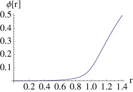
For , the zero temperature solution not only has Poincare symmetry but approaches near the horizon, and is just a Poincare horizon. The leading order corrections can be found analytically and depend on a parameter which is a function of , but stays small (). Explicitly,
| (10) | |||
| (11) | |||
| (12) |
where
| (13) |
| (14) |
Although the curvature remains finite, derivatives of the curvature diverge at unless . FIG. 2 shows the solution for and for a choice of which is close to the value where Reissner-Nordstrom AdS is stable. One sees that dips down and has a local minimum at a value . As , vanishes at this local minimum which becomes the horizon of the extremal Reissner-Nordstrom AdS black hole.
For ( and ), the zero temperature solution near the horizon is
| (15) |
| (16) |
where
| (17) |
and is adjusted to satisfy the boundary condition at infinity. The near horizon metric is (after rescaling )
| (18) |
One clearly sees the Poincare symmetry (but not the conformal symmetry) in this case. There is a rather mild null curvature singularity at .

III Dirac equation
The Dirac action is
| (19) |
where we are using the conventions of [46]. The coupling could be replaced by a more general function of . We will set for now except to discuss its effects briefly below.
As discussed in section I.1 if the charge of the scalar is such that then we can add to this
| (20) |
where the charge conjugation matrix is
| (21) |
This term is essentially a Majorana mass term. There are two terms because there are two Majorana spinors in the bulk (or Weyl spinors) and these can have independent masses.
In the case of odd numbers of bulk dimensions, there is no and this term does not exist. This matches the fact that in odd numbers of bulk dimensions, a single Dirac spinor in the bulk describes a chiral fermion operator in the boundary theory [47]; such a fermion cannot be paired with itself in a rotation-invariant way. The analogous coupling in odd bulk dimensions requires two Dirac fermions. That this is possible can be seen by dimensionally reducing a theory with an even number of bulk dimensions on a circle. We will not discuss this in detail here.
Now we study the Dirac equation in more detail. It turns out that the same simplification that appeared in the RN background occurs for the more general metric (8). Very briefly, the form of the spin connection
| (22) |
implies that
| (23) |
so we can rescale and remove the spin connection completely. The new action is
| (24) |
where with no appearance of the spin connection.
The Dirac equation following from is
| (25) |
Expand this into Fourier modes with :
| (26) |
To get any further we must specify a basis of Dirac matrices. We focus on , that is, a dimensional bulk. We choose a basis of bulk Gamma matrices as in [17],
| (28) | |||||
such that and which fixes the charge conjugation matrix to be . This basis has the features that (with and ) the Dirac equation is completely real.
We will now split the 4-component spinors into two 2-component spinors where the index is the Dirac index of the boundary theory. Then
| (29) | |||
| (30) |
where44 4 The frequency is measured from the chemical potential.
| (31) |
We see that the term mixes with (and with ) - this is the mixing that will most interest us, because for the RN background these two fields have coincident Fermi surfaces (at ). Setting (30) becomes
| (32) |
where
| (33) |
are the bulk analogs of the Nambu-Gork’ov spinor.55 5 The index on is the boundary theory Dirac index. For the rest of this section (III) for simplicity of the discussion we will concentrate mostly on one of these: . In section (IV) we will give results for . We see explicitly from (32) that for a general black hole background in the absence of mixing () the spectrum of compared to the spectrum of is a reflection about the axis. This is crucial for generically generating gapped states for non-zero .
We have set both to make the analysis easier and because turning on both and implies that some discrete symmetry of the boundary theory is broken.
For completeness, we record the Dirac equation with . In this case, the mixing would be between and with the equation being
| (34) |
where . Because the differential operators in the diagonal entries above are evaluated with opposite , the two mixed components will not have coincident spectra at (see Figure 5 of [17] to see this in the RN background). As such there will only be eigenvalue repulsion if there is some accidental eigenvalue crossing, and this will generically occur away from . This should be contrasted with the mixing discussed above.
III.1 Boundary conditions
As reviewed in section 2, many of the solutions found in [44] have an emergent Poincare symmetry in the deep IR, and some even have emergent conformal symmetry. For now we will mainly consider the latter case in which the solution approaches near the horizon. To determine the IR boundary conditions for the spinor appropriate for the retarded Green’s function, we consider the Dirac equation in the far IR region, where the metric is just pure with no electric field and zero chemical potential:
| (35) |
The speed of light in the dual IR CFT is . The most relevant terms in the Dirac equation close to the Poincare horizon are , with
| (36) |
Very generally, the off-diagonal terms are subdominant, by arguments given in [44] in the discussion of the Schrödinger potential for the optical conductivity: the relative magnitude of the off-diagonal term to the terms appearing in (36) is which must generally vanish on the horizon.
Because of the diagonal form of (36), we can construct a basis of ingoing solutions by considering and separately. As is familiar from zero-temperature , the character of the boundary conditions depends on the sign of . To begin with we will work outside the light cone where is spacelike. Here the behavior of the solutions is normalizable and non-normalizable. We will pick the one which is normalizable at :
| (37) | |||
| (38) | |||
| (39) |
is an eigenvector of the matrix in (36). This now allows us to formulate the general incoming boundary conditions in order to compute retarded correlators. We simply use the prescription to define how to continue the branch cuts in (37) to timelike . That is, we take .
For the other component we can simply take in (37),
| (40) | |||
| (41) | |||
| (42) |
and again for timelike in (40) we continue 66 6 Beware the following confusion: because there is a complex conjugation on , one might expect this to switch the sign of the . This is not the case because we should think of analytically continuing ; this procedure preserves the incoming boundary conditions. In the absence of the mixing, the two solutions of the Dirac equation (32) for specified by the IR behavior compute the Green’s functions for the two boundary fermion operators, and .
Now we consider the boundary conditions at the boundary of the UV . This will tell us how to read off the field theory correlators. The mixing term is again subdominant at the UV boundary, so that the asymptotic behavior is the same as usual:
| (43) |
and similarly for . The boundary retarded Green’s function is: 77 7 The minus signs appearing in front of come from the fact that is the source for where the minus sign is from anti-commuting this (Grassman valued) source in the boundary theory action so that it is in the correct order and the action is real.
| (44) |
The definition of the Green’s functions appearing above is:
| (45) |
Note that the spectral densities (which should be positive by unitarity) are and .
More generally including the analysis for the above matrix (44) will fit into the Lorentz covariant correlator which is a matrix (recall that this is for ):
| (46) |
where and where the boundary theory charge conjugation matrix can be shown to be . Note that all the entries in this matrix will be non-zero if both are turned on.
III.2 Evolution equation
It turns out there is a super nice way to package the above linear differential equation into a non-linear evolution equation, in the spirit of the evolution equations considered in [48] and used in [47, 16]. This is useful for identifying the Fermi surfaces numerically, because although the spinor components vary greatly with , their ratios, which appear in the evolution equation, remain order one.
Define the following matrices:
| (47) | |||||
| (49) |
Then one can write the following evolution equation:
| (50) | |||
The boundary conditions on this matrix at the IR horizon and the UV boundary become respectively:
| (51) | |||||
| (52) |
Note that when the evolution equation preserves the diagonal form of the initial condition in the IR.
This method runs into difficulty if becomes non-invertible at finite ; this happens for the multi-node boundstates associated with secondary Fermi surfaces.
IV Results: Bound states outside the emergent light cone
IV.1 No mixing
We start by looking at so there is no mixing. We will concentrate on the field (from which we can reflect about to generate . ) Note that we are now switching relative to the discussion of the previous section - all results in this section will be for the Nambu Gork’ov spinor . The reason being the primary Fermi surface in the RN background (the one with largest ) makes its appearance in the Green’s function for [17]. We are interested in understanding the fate of this primary Fermi surface in the condensed phase.
Now since the initial conditions are real for spacelike and the Dirac equation for in the absence of mixing is real, the spectral functions should be zero outside the emergent IR lightcone. This is true up to delta functions which can appear because the real part of the Green’s function has a pole which becomes a delta function in the imaginary part thanks to Kramers-Kronig. These are bound states of the Dirac equation since they are normalizable at the IR horizon and at the UV boundary. They will represent infinitely long lived fermion states in the field theory.
For now we will look for these states in a small set of the zero temperature hairy black holes constructed in [44] and reviewed above. We will concentrate on the case with zero scalar potential energy () with general charge for the scalar. In this case and the speed of light in the IR CFT can be found numerically, see FIG. 1.
The fermion charge88 8 There is a factor of two difference in the normalization of the charges for both scalars and spinors in [16] (LMV) compared to [44] (HR) – they are related by . We will work with the normalization throughout. will be constrained by gauge invariance to be , so that the term can be added later. The mass of the fermion is a priori independent of the mass of the scalar. We work with for numerical convenience. It will be interesting to look at small charges close to the critical charge where the critical temperature and . For the RN black hole is stable, and as can be seen from FIG. 2, the superconducting groundstate approaches the RN solution. In this limit the spectral densities should look more and more similar to the ones of the RN black hole, which we have a good handle on. Indeed, for reference, we know that there is a Fermi surface in the RN black hole for and when with IR scaling exponent .
FIG. 3 shows the location of these states for different in these zero temperature superconducting backgrounds.

IV.2 Mixing
The stable gapless () excitations we have found in FIG. 3 seem rather surprising in a strongly coupled theory. We now demonstrate that turning on (and keeping ) the stable excitations studied above develop a gap. The reason for this can be simply understood by the general arguments of eigenvalue repulsion. Since the positive frequency modes mix with the negative frequency modes (at the same ) the repulsion occurs when .
More carefully, we can study the Dirac equation with mixing. Because the initial conditions (37) and (40) for spacelike are real one might expect that again the spectral functions are zero except for delta functions. This is a little subtle because the Dirac equation (32) is real except for the term. However it turns out that despite this, the spectral functions are still zero. We can see this in two ways. Firstly, the spectral functions are the difference in the retarded and advanced Green’s functions (this is more general than the imaginary part of the retarded function). For spacelike these two Green’s functions are calculated with the same Dirac equation and the same initial conditions (the difference comes from the prescription when going to .) Hence here and the spectral function is zero except for on bound states.
Secondly, the evolution equation (50) for spacelike preserves the following form of the Green’s function matrix (recall we have switched relative to (50) ):
| (53) |
Hence the spectral densities for are zero. The phase of is arbitrary since we can change it by rephasing the operator , hence it cannot matter for the spectral density of .
To find the bound state in this situation we should look for places where at the boundary. Note that for so indeed this is a well defined problem. This delta function will appear in all spectral densities. The residue however will be different in each component. We concentrate on because this is what should be accessible to photoemission “experiments”. The results are given in FIG. 4 and FIG. 5.


We can learn something from perturbation theory in . The splitting is determined by the eigenvalues of the matrix
| (54) |
where
| (55) |
( was defined in [17], appendix C) and
| (56) |
where denotes the boundstate wavefunction in the basis Thinking of the Dirac equation as a Schrödinger problem, this matrix is the perturbation Hamiltonian in the degenerate subspace.
The fact that at , the up and down boundstates are the same implies that and ); the eigenvalues of are therefore
| (57) |
Looking for low-energy boundstates with fixed then requires these eigenvalues to vanish, which occurs when , i.e. when .
IV.3 Luttinger-like behavior near the lightcone
To understand what’s happening at , we consider the Schrödinger form of the wave equation, where the role of the energy eigenvalue is played by . For simplicity (and because the pictures are nicer) we draw the potentials for the case of a charged scalar probe (not to be confused with the charged scalar which is condensing.) For further details, see Appendix B of [17].


The physics of the IR lightcone is visible in FIG. 6. In the RN background (right plot), turning on any nonzero frequency opens up a bottomless pit in the effective potential leading into the region where the tortoise coordinate . Therefore, in the RN groundstate there are no infinitely-stable quasiparticles with nonzero frequency. On the other hand, in the superconducting groundstate, the limiting value of the effective potential as is . Therefore, there is a threshold frequency below which the IR limit of the Schrödinger potential remains above the boundstate energy. More precisely, there will be a normalizable bound state close to the boundary as long as the energy () is less than the limiting value . Beyond this the bound state enters the light-cone and is no longer a stable quasi particle.
The fact that we see a stable particle below the continuum is qualitatively what one expects for systems with a gap . For energies , one excites a single quasiparticle which is stable since there is nothing for it to decay into. Only at energies above does one start to see a continuum.
The spectral density near the lightcone, and in particular the width of the quasiparticle after it enters the lightcone can be computed by matching between the regions in UV and IR as in [17, 44]. The size of the overlap region is controlled by the quantity which should be small in units of the chemical potential. In the notation of [17], the result for the Green’s function is of the form
| (58) |
where are real99 9 They are only real if we take which we can do without loss of generality. data associated with the UV region, and is the IR CFT Green’s function to be discussed below. If there is mixing between positive and negative frequency modes then are matrices in the basis of the Nambu-Gork’ov spinor. They are smooth (analytic) functions of so the leading non analytic behavior in is from . For purposes of exposition we will describe the results for a probe scalar field in parallel to that of the spinor. We will leave details of the spinor calculation to Appendix A.
For a probe scalar, the IR CFT Green’s function is
| (59) |
The quantities are related to the IR CFT scaling dimension of the boundary operator by , and are determined by studying the behavior of the field at the UV boundary of the IR region in (35). They are given by
| (60) |
where (the subscript is for ‘condensed’ and is intended to distinguish this object from the analogous IR CFT scaling dimension in the region of RN [17]). Notice that the IR CFT scaling dimension depends on the coupling .
For the probe spinor the IR CFT Green’s function appearing in (58) is
| (61) |
For the spinor case the relation between and is,
| (62) |
see Appendix A for more details.
We can extract two interesting statements from these calculations. From the form of (58) (and in particular the reality of ) we learn that at generic (but small so that this matching applies),
| (63) |
The dependence of on has the following consequence. In the last plot of FIG. 4, one can see that the coupling to the condensate is also suppressing the incoherent spectral weight inside the lightcone. This is because the IR CFT dimension is becoming large as we make large.
Finally, if we look near a quasiparticle pole, which close to the light-cone occurs when , we see that the imaginary part of the location of the pole is determined by the IR CFT Green’s function. This determines the width of the resonance as it enters the lightcone. The result is that the width behaves as
| (64) |
for the scalar and spinor respectively, which can be compared to the behavior in FIG. 4.1010 10 Actually we need to be more careful for the case (for the spinor.) Here (64) should be replaced by, .
We emphasize that there are two mechanisms which suppress the spectral weight: one sets it exactly zero (except for delta functions) outside the light cone. This is a property of IR behavior of the background geometry. The other mechanism suppresses the weight independently of the momentum (this is a numerical observation visible from the dashed blue lines in FIG. 5), and depends on the scalar-spinor coupling. This mechanism generates the gap for the quasiparticle peak, and can be understood in terms of the dependence of the effective IR scaling dimension of the fermion operator on as in the previous discussion. The latter mechanism also affects physics at whereas the lightcone mechanism does not.
V Discussion
We should make a few remarks about the effects of other possible couplings between the bulk spinor and scalar. The coupling
| (65) |
is possible whatever the charge of the spinor and scalar. By the argument given in section I.1, the Green’s function for the system with near should have only one pole (whose location may however be dramatically affected by the couplings ), and the effects of the interaction (65) cannot be interpreted as mixing of particle and hole states. As the coupling is varied, it is easy to be fooled into thinking that there is a gap even when there is not, when looking at energy distribution curves because the Fermi momentum moves with .
As observed first in [41] increasing the mass of the effective field in the IR (which can be achieved by either including the above coupling or changing the UV mass: ) can lead to poles which never reach the axis and may be interpreted as gapped. This mechanism for removing low-energy spectral weight (which happens because increasing pushes up the effective Schrödinger potential for the Dirac equation) is qualitatively different from the mixing described in the previous sections. It is analogous to adding a relativistic mass to particles and anti-particles in a relativistic field theory at non-zero chemical potential. The gap in this situation is around and does not generically produce a gap at . This should be compared to the gap from the coupling which is like adding a mass to particles and holes (absence of particles) about the Fermi surface at .
It was shown in [44] that the zero temperature superconductors we have studied here do not have a hard gap in the optical conductivity: The real part of the conductivity remains nonzero (although typically exponentially small) at low frequency and . Despite this fact, one might have wondered whether such a hard gap in the conductivity exists for the fermionic probes that we study in this paper. The existence of a non-zero spectral weight around the origin of FIG. 4 suggests that this is not the case; however, to see this effect in the conductivity it would be necessary compute a correction as in [26].
It would be interesting to understand better what property of the boundary theory is reflected by the presence of the coupling, which is required to produce an actual gap in the fermion response. One clue is that its presence specifies the ‘intrinsic parity’ of the dual operator, i.e. the dual operator acquires an interesting phase under a parity transformation. Realizing string vacua where this coupling is nonzero would probably be valuable.
So far we have considered the fermion spectral function at zero temperature. FIG 7 shows what happens as one raises the temperature. The temperatures shown are much less than . As , the condensate goes to zero, so its coupling to the fermions goes to zero and the gap disappears. Actually, the thermal broadening of the peak makes the gap disappear at about . In the opposite limit, as , the width of the peak vanishes rapidly. It appears to vanish faster than a power law, but the general temperature dependence deserves further investigation.

We close with a few comparisons with real phenomena. Here we make a simple observation which follows from the sharpness of the peaks in the ‘no man’s land’ regime (i.e. outside the IR light cone). This regime is induced by the superconducting order. This means that if we start at high temperature in the normal phase with some Fermi surface without stable quasiparticles (like say a marginal Fermi liquid case, in the notation of [17]), and cool into the superconducting phase, sharp quasiparticle peaks appear, at least for not too big. This matches a mysterious piece of cuprate phenomenology: in the normal phase, photoemission experiments show no stable quasiparticle peak, but a coherent peak emerges in the superconducting phase (see e.g. figure 47 of the review [50]). From the gravity point of view, this is happening because the scalar condensate is removing the region which was responsible for the finite lifetime of the holographic quasiparticles [17]: this is the gravity statement that the condensate is lifting the many gapless excitations into which the quasiparticle could decay. The mechanism for the stability of these excitations is very similar to the recent holographic explanation [51] of the critical velocity in a (holographic) superfluid below which there is no drag, and above which energy is dissipated by the creation of IR unparticles.
This similarity can be made more precise. In a BCS superfluid, the decay of the quasiparticles can be mediated by emission of a Goldstone boson (this mode is eaten in a superconductor, and the following effect is absent). It can happen that this decay is kinematically forbidden: the decay cannot happen if the group velocity of the quasiparticle is larger than the speed of sound (see appendix B of [52]). In our system, the quasiparticles develop a finite lifetime when they can decay into the modes of the IR CFT dual to the IR region. These modes are distinct from the Goldstone mode (which is apparently hidden by powers of ), but the effect is the same.
The energy distribution curves ( at fixed ) shown in FIG. 5 exhibit another feature in common with ARPES measurements on the cuprates, namely the so-called ‘peak-dip-hump’ structure: in addition to the quasiparticle peak, one sees a broad maximum at larger . This is a consequence of the IR lightcone. Over-ambitiously, if this were the correct interpretation, the location of the hump would give a measurement of the speed of light of the quantum critical theory.
Acknowledgements
We thank Nabil Iqbal and Hong Liu for collaboration on related matters. We thank S. Hartnoll, S. Kachru, A. Ludwig, M. Mulligan, Y. Nishida, S. Sachdev, T. Senthil, B. Swingle, A. Yarom, W. Zwerger and many of the participants of the “Quantum Criticality and the AdS/CFT Correspondence” miniprogram at the KITP for useful discussions. Work supported in part by funds provided by the U.S. Department of Energy (D.O.E.) under cooperative research agreement DE-FG0205ER41360. The research was supported in part by the National Science Foundation under Grant No. NSF PHY05-51164 and the UCSB Physics Department. G. H. and M. R. were supported in part by NSF grant PHY-0855415.
Appendix A Spinor in the IR region
The Dirac equation in the IR region including the mixing term is
| (66) |
Now to solve this we employ the following basis rotation . Then the Dirac equation takes the form:
| (67) | |||
| (68) |
where
| (69) |
We can now block diagonalize this equation into two independent Dirac equations. We make the following basis rotation:
| (70) |
Here,
| (71) | |||
| (72) | |||
| (73) |
where determines the conformal dimension of the spinor in the IR region. These Dirac equations are then exactly that of a spinor in with mass . The (two) general incoming solutions can be found, and at the boundary of this IR , a basis for these solutions behaves like
| (74) |
| (75) |
where the IR Green’s function for a spinor is
| (76) |
References
- [1] T. Holstein, R. E. Norton and P. Pincus, “de Haas-van Alphen Effect and the Specific Heat of an Electron Gas,” Phys. Rev. B 8, 2649 (1973).
- [2] M. Y. Reizer, “Relativistic effects in the electron density of states, specific heat, and the electron spectrum of normal metals,” Phys. Rev. B 40, 11571 (1989).
- [3] G. Baym, H. Monien, C. J. Pethick, and D. G. Ravenhall, “Transverse interactions and transport in relativistic quark-gluon and electromagnetic plasmas,” Phys. Rev. Lett. 64 (1990) 1867.
- [4] J. Polchinski, “Low-energy dynamics of the spinon gauge system,” Nucl. Phys. B 422, 617 (1994) arXiv:cond-mat/9303037.
- [5] C. Nayak and F. Wilczek, “Non-Fermi liquid fixed point in (2+1)-dimensions,” Nucl. Phys. B 417, 359 (1994) arXiv:cond-mat/9312086, “Renormalization group approach to low temperature properties of a non-Fermi liquid metal,” Nucl. Phys. B 430, 534 (1994) arXiv:cond-mat/9408016.
- [6] B. I. Halperin, P. A. Lee and N. Read, “Theory of the half filled Landau level,” Phys. Rev. B 47, 7312 (1993).
- [7] B. L. Altshuler, L. B. Ioffe and A. J. Millis, “On the low energy properties of fermions with singular interactions,” arXiv:cond-mat/9406024.
- [8] T. Schafer and K. Schwenzer, “Non-Fermi liquid effects in QCD at high density,” Phys. Rev. D 70, 054007 (2004) arXiv:hep-ph/0405053.
- [9] D. Boyanovsky and H. J. de Vega, “Non-Fermi liquid aspects of cold and dense QED and QCD: Equilibrium and non-equilibrium,” Phys. Rev. D 63, 034016 (2001) arXiv:hep-ph/0009172;
- [10] S. S. Lee, “Low energy effective theory of Fermi surface coupled with U(1) gauge field in 2+1 dimensions,” arXiv:0905.4532 [cond-mat.str-el].
- [11] P. A. Lee and N. Nagaosa, “Gauge theory of the normal state of high-Tc superconductors,” Phys. Rev. B 46, 5621 (1992).
- [12] Y. B. Kim, A. Furusaki, P. A. Lee, and X-G. Wen, “Gauge-invariant response functions of fermions coupled to a gauge field,” Phys. Rev. B 50, 17917 (1994); Y. B. Kim, P. A. Lee, and X-G. Wen, “Quantum Boltzmann equation of composite fermions interacting with a gauge field” Phys. Rev. B 52, 17275 (1995).
- [13] V. Oganesyan, S. Kivelson, E. Fradkin, “Quantum Theory of a Nematic Fermi Fluid,” Phys. Rev. B 64, 195109 (2001), arXiv:cond-mat/0102093v2 [cond-mat.str-el].
- [14] C. P. Nave and P. A. Lee, “Transport properties of a spinon Fermi surface coupled to a U(1) gauge field,” Phys. Rev. B 76, 235124 (2007).
- [15] S. S. Lee, “A Non-Fermi Liquid from a Charged Black Hole: A Critical Fermi Ball,” arXiv:0809.3402 [hep-th].
- [16] H. Liu, J. McGreevy and D. Vegh, “Non-Fermi Liquids from Holography,” arXiv:0903.2477 [hep-th].
- [17] T. Faulkner, H. Liu, J. McGreevy and D. Vegh, “Emergent Quantum Criticality, Fermi Surfaces, and Ad,” arXiv:0907.2694 [hep-th].
- [18] M. Cubrovic, J. Zaanen and K. Schalm, “Fermions and the AdS/CFT correspondence: quantum phase transitions and the emergent Fermi-liquid,” arXiv:0904.1993 [hep-th].
- [19] S. J. Rey, “String Theory on Thin Semiconductors,” Progress of Theoretical Physics Supplement No. 177 (2009) pp. 128-142; arXiv:0911.5295 [hep-th].
- [20] J. M. Maldacena, “The large N limit of superconformal field theories and supergravity,” Adv. Theor. Math. Phys. 2, 231 (1998); [arXiv:hep-th/9711200]; E. Witten, “Anti-de Sitter space, thermal phase transition, and confinement in gauge theories,” ibid. 505 (1998); [arXiv:hep-th/9803131]; S. S. Gubser, I. R. Klebanov and A. M. Polyakov, “Gauge theory correlators from non-critical string theory,” Phys. Lett. B 428, 105 (1998). [arXiv:hep-th/9802109].
- [21] S. Sachdev and M. Mueller, “Quantum Criticality and Black Holes,” arXiv:0810.3005 [cond-mat.str-el].
- [22] S. A. Hartnoll, “Lectures on Holographic Methods for Condensed Matter Physics,” arXiv:0903.3246 [hep-th].
- [23] C. P. Herzog, “Lectures on Holographic Superfluidity and Superconductivity,” J. Phys. A 42 (2009) 343001 [arXiv:0904.1975 [hep-th]].
- [24] J. McGreevy, “Holographic Duality with a View Toward Many-Body Physics,” arXiv:0909.0518 [hep-th].
- [25] C. M. Varma, P. B. Littlewood, S. Schmitt-Rink, E. Abrahams and A. E. Ruckenstein, “Phenomenology of the normal state of Cu-O high-temperature superconductors,” Phys. Rev. Lett. 63, 1996 (1989).
- [26] T. Faulkner, N. Iqbal, H. Liu, J. McGreevy and D. Vegh, “Transport by Holographic non-Fermi Liquids” to appear.
- [27] S. S. Gubser, “Breaking an Abelian gauge symmetry near a black hole horizon,” Phys. Rev. D 78, 065034 (2008) [arXiv:0801.2977 [hep-th]].
- [28] S. A. Hartnoll, C. P. Herzog and G. T. Horowitz, “Building a Holographic Superconductor,” Phys. Rev. Lett. 101, 031601 (2008) [arXiv:0803.3295 [hep-th]], “Holographic Superconductors,” JHEP 0812, 015 (2008) [arXiv:0810.1563 [hep-th]];
- [29] J. G. Bednorz and K. A. Müller, ”Possible high Tc superconductivity in the Ba-La-Cu-O system,” Z. Physik, B 64 (1), 189Ð193.
- [30] P. Gegenwart, Q. Si and F. Steglich, “Quantum criticality in heavy-fermion metals,” Nature Physics 4, 186 (2008).
- [31] C. P. Herzog, I. R. Klebanov, S. S. Pufu and T. Tesileanu, “Emergent Quantum Near-Criticality from Baryonic Black Branes,” arXiv:0911.0400 [hep-th].
- [32] S. S. Gubser and F. D. Rocha, “Peculiar Properties of a Charged Dilatonic Black Hole in ,” arXiv:0911.2898 [hep-th].
- [33] K. Goldstein, S. Kachru, S. Prakash and S. P. Trivedi, “Holography of Charged Dilaton Black Holes,” arXiv:0911.3586 [hep-th].
- [34] This argument for the genericity of charge- bosons is due to Shamit Kachru.
- [35] F. Denef and S. A. Hartnoll, “Landscape of superconducting membranes,” Phys. Rev. D 79, 126008 (2009) [arXiv:0901.1160 [hep-th]].
- [36] E. Silverstein, “TASI/PiTP/ISS lectures on moduli and microphysics,” arXiv:hep-th/0405068; F. Denef, M. R. Douglas and S. Kachru, “Physics of string flux compactifications,” Ann. Rev. Nucl. Part. Sci. 57, 119 (2007) [arXiv:hep-th/0701050]; M. R. Douglas and S. Kachru, “Flux compactification,” Rev. Mod. Phys. 79, 733 (2007) [arXiv:hep-th/0610102]; M. Grana, “Flux compactifications in string theory: A comprehensive review,” Phys. Rept. 423, 91 (2006) [arXiv:hep-th/0509003]; F. Denef, “Les Houches Lectures on Constructing String Vacua,” arXiv:0803.1194 [hep-th].
- [37] N. Arkani-Hamed, L. Motl, A. Nicolis and C. Vafa, “The String Landscape, Black Holes and Gravity as the Weakest Force,” JHEP 0706 (2007) 060 [arXiv:hep-th/0601001].
- [38] X. J. Zhou, T. Cuk, T. Devereaux, N. Nagaosa, Z.-X. Shen, “Angle-Resolved Photoemission Spectroscopy on Electronic Structure and Electron-Phonon Coupling in Cuprate Superconductors,” Handbook of High-Temperature Superconductivity: Theory and Experiment, edited by J. R. Schrieffer, (Springer, 2007), Page 87-144, [arXiv:cond-mat/0604284].
- [39] J. C. Campuzano, M. R. Norman and M. Randeria, “Photoemission in the High Tc Superconductors,” in Handbook of Physics: Physics of Conventional and Unconventional Superconductors, edited by K. H. Bennemann and J. B. Ketterson, (Springer Verlag, 2004); [arXiv:cond-mat/0209476].
- [40] J. W. Chen, Y. J. Kao and W. Y. Wen, “Peak-Dip-Hump from Holographic Superconductivity,” arXiv:0911.2821 [hep-th].
- [41] S. S. Gubser, F. D. Rocha and P. Talavera, “Normalizable Fermion Modes in a Holographic Superconductor,” arXiv:0911.3632 [hep-th].
- [42] A. Adams, to appear.
- [43] M. G. Alford, A. Schmitt, K. Rajagopal and T. Schafer, “Color Superconductivity in Dense Quark Matter,” Rev. Mod. Phys. 80 (2008) 1455 [arXiv:0709.4635 [hep-ph]].
- [44] G. T. Horowitz and M. M. Roberts, “Zero Temperature Limit of Holographic Superconductors,” JHEP 0911 (2009) 015 [arXiv:0908.3677 [hep-th]].
- [45] S. S. Gubser and A. Nellore, “Ground States of Holographic Superconductors,” arXiv:0908.1972 [hep-th].
- [46] J. Polchinski, String Theory, Vol. 2, Appendix B.
- [47] N. Iqbal and H. Liu, “Real-Time Response in AdS/CFT with Application to Spinors,” Fortsch. Phys. 57 (2009) 367 [arXiv:0903.2596 [hep-th]].
- [48] N. Iqbal and H. Liu, “Universality of the Hydrodynamic Limit in AdS/CFT and the Membrane Paradigm,” Phys. Rev. D 79 (2009) 025023 [arXiv:0809.3808 [hep-th]].
- [49] F. Denef, S. A. Hartnoll and S. Sachdev, “Quantum Oscillations and Black Hole Ringing,” arXiv:0908.1788 [hep-th]; “Black Hole Determinants and Quasinormal Modes,” arXiv:0908.2657 [hep-th].
- [50] A. Damascelli, Z. Hussain, Z.-X. Shen, “Angle-resolved photoemission studies of the cuprate superconductors,” Rev. Mod. Phys. 75, 473 - 541 (2003).
- [51] S. S. Gubser and A. Yarom, “Pointlike Probes of Superstring-Theoretic Superfluids,” arXiv:0908.1392 [hep-th].
- [52] R. Haussmann, M. Punk, W. Zwerger, “Spectral Functions and rf Response of Ultracold Fermionic Atoms,” to appear in Phys. Rev. A, arXiv:0904.1333v2 [cond-mat.quant-gas].