,,
Statistics of leaders and lead changes in growing networks
Abstract
We investigate various aspects of the statistics of leaders in growing network models defined by stochastic attachment rules. The leader is the node with highest degree at a given time (or the node which reached that degree first if there are co-leaders). This comprehensive study includes the full distribution of the degree of the leader, its identity, the number of co-leaders, as well as several observables characterizing the whole history of lead changes: number of lead changes, number of distinct leaders, lead persistence probability. We successively consider the following network models: uniform attachment, linear attachment (the Barabási-Albert model), and generalized preferential attachment with initial attractiveness.
pacs
64.60.aq, 05.40.–a, 89.75.Hc, 89.75.–k1 Introduction
One of the most salient features of complex networks [1, 2, 3, 4] is their scalefreeness: they usually exhibit a broad degree distribution falling off as a power law:
| (1.1) |
with , so that the mean degree is finite. Growing networks with preferential attachment, such as the Barabási-Albert model [5], brought a natural explanation for the ubiquity of the observed scalefreeness. These model systems also provide a playground to investigate other, more refined features of networks and other random growing structures. In this work we focus our attention onto leaders and lead changes. Luczak and Erdös [6] already describe as a kind of a race the growth of connected components in the Erdös-Rényi model for random graphs [7], and refer to the largest component as the leader. This terminology was then introduced in the physics literature by the pioneering work of Krapivsky and Redner [8], in concomitance with the growing interest in social networks. As suggested by these authors, as the degree of a node may quantify the wealth of a corporation or the popularity of a person, it is natural to investigate questions such as How does the identity of the leader change in the course of time? What is the probability that a leader retains the lead as a function of time?
The first and most natural of all quantities pertaining to this area is the degree of the leader, i.e., the largest of the node degrees at time . This quantity is known to play a central rôle in finite-size effects on the degree statistics. The following picture has indeed progressively emerged [9, 10, 11]. For a large but finite scalefree network at time , the ‘stationary’ power law (1.1) is cutoff at some time-dependent scale , which is of the order of the typical value of the largest degree . The latter can in turn be estimated, at least as a first approximation, by means of a well-known argument of extreme-value statistics [12]: the stationary probability for the degree to be larger than is of order . In the scalefree case, the largest degree is thus predicted to grow as a power law:
| (1.2) |
This growth law is subextensive, as implies .
The goal of the present paper is to provide a systematic study of the distribution of the largest degree and of other quantities related to leaders and lead changes in growing networks, thus improving and generalizing most of the results presented in [8, 13]. We consider network models where a new node enters at each time step, so that nodes can be identified by an index equal to the time they enter the network. We adopt the setup and some of the notations of our earlier work [11], devoted to finite-size effects on the degree statistics. The quantities to be investigated concern either the leader at a given time or the whole history of lead changes:
The largest degree at time is by definition the largest of the degrees of all the nodes at time (:
| (1.3) |
We will investigate both the mean value of and its full distribution.
A co-leader at time is any node whose degree is equal to the largest degree . We denote by the number of co-leaders at time . As the node degrees are integers, it is not rare that the largest degree (or any other value) is simultaneously shared by two or more nodes.
The leader at time is the node among the co-leaders whose degree reached the value first. This definition is already used in [6]. We denote by the index of the leader at time . Initial conditions will be such that the first node is the first leader.
There is a lead change at time if the leader at time is different from that at time . We call a lead any period of time between two lead changes. We denote by the number of leads up to time . In other words, the number of lead changes up to time is .
Finally, some lead changes bring to the lead a node that has already been the leader in the past, whereas some other changes promote a newcomer. We denote by the number of distinct leaders up to time . We also introduce the lead persistence probability as the probability that there is a single leader up to time .
We will consider network models where node attaches to a single earlier node (), with a prescribed attachment probability:
Uniform attachment (UA) (Section 2): the attachment probability is independent of the node, i.e., uniform over the network. This model has a geometric degree distribution: it is therefore not scalefree. Its analysis however allows a detailed introduction of key concepts and quantities, such as the discussion of the ‘stationary extreme-value statistics’ approach, given in Section 2.1.
Barabási-Albert (BA) model (Section 3): the attachment probability is proportional to the degree of the earlier node. This well-known model [5] is scalefree, with exponents and .
General preferential attachment (GPA) (Section 4): the attachment probability is proportional to the sum of the degree of the earlier node and of a constant . This parameter, representing the initial attractiveness of a node [9], yields the continuously varying exponents and .
Finally, for each of these models, it will be interesting to simultaneously analyze data for two different initial conditions [11]:
Case A. Node 1 appears at time with degree . At time node 2 attaches to node 1, so that . At time node 3 attaches a priori either to node 1 or to node 2 with equal probabilities. We choose to attach node 3 to node 1, obtaining thus , whereas , so that node 1 is the first leader. This is the initial condition used e.g. in [8].
Case B. Node 1 appears at time with degree . This amounts to saying that the first node is connected to a root, which does not belong to the network. It is natural to represent this connection by half a link. At time node 2 attaches to node 1. We thus have and , so that node 1 is again the first leader.
The sum of the degrees of all the nodes at time equals twice the number of links in the network [11, Eq. (1.3)]:
| (1.4) |
with and . Here and in the following, the superscripts and denote a result which holds for a prescribed initial condition (Case A or Case B).
2 The uniform attachment (UA) model
In the uniform attachment model, each new node attaches to any earlier node () with uniform probability:
| (2.1) |
2.1 Largest degree
The stationary degree distribution in the UA model has a geometric form:
| (2.2) |
It is useful to recall the derivation of this result. The distribution of the degree of node at time obeys the recursion [11, Eq. (2.11)]
| (2.3) |
with for . The distribution of the degree of an arbitrary node,
| (2.4) |
therefore obeys the recursion
| (2.5) |
Finally, the stationary degree distribution (corresponding to at fixed ) obeys the recursion
| (2.6) |
which easily yields (2.2).
Applying the extreme-value argument recalled in the Introduction to the geometric distribution (2.2), we recover the logarithmic growth of the largest degree [8]:
| (2.7) |
One could be tempted to go further along this line of reasoning and to assert that the full distribution of the largest degree can be derived, asymptotically for large, from the stationary extreme-value statistics approach. This consists in modeling as the largest of independent variables drawn from the stationary distribution . As already suggested in [13], this approach cannot however be exact for the following three reasons, in order of increasing importance:
- (1)
Sum rule. The degrees are not independent random variables, as they obey the sum rule (1.4). This condition is however harmless for large , as it imposes a single constraint on variables.
- (2)
Finite-size (i.e., finite-time) effects. The distribution of the degree of a node at time does not coincide with its stationary value . It is indeed affected by finite-size effects, which have been studied in detail in [11]. As recalled in the Introduction, these effects become important for . Finite-size effects may therefore alter the statistics of the largest degree.
- (3)
Correlation between degree and index. The degrees of the nodes are not identically distributed. In particular, older nodes typically have larger degrees. Their distribution may depend rather strongly on the node index , especially for .
Points (2) and (3) raise rather delicate issues, which deserve a specific investigation for each model. The UA model is a rather fortunate case where the above points are to a large extent under control [11, Sec. 2]. Concerning point (3), the dependence of the distribution on the index is rather weak. We have for instance [11, Eq. (2.4)]
| (2.8) |
for and large. The leading logarithmic growth of this expression is independent of the node index , which only enters the ‘finite part’ of the logarithm. Concerning point (2), i.e., finite-size effects, the ratio between the true distribution for finite and its stationary counterpart stays approximately equal to unity, before it drops to zero in a range of degrees scaling as around . The prefactor 2 of this estimate is larger than the prefactor of the law (2.7), so that the distribution is expected to be closer and closer to the stationary one for degrees near the mean largest degree. We are therefore tempted to argue that the ‘stationary extreme-value statistics’ approach, or stationary approach for short, provides a good description of the distribution of the largest degree and of related observables, which may even yield exact asymptotic results, at least for quantities which are only sensitive to the leading logarithmic growth of expressions like (2.8), and not to their ‘finite parts’.
The statistics of extremes for i.i.d. integer variables is reviewed in Appendix A, with emphasis on geometric distributions. The exact distribution of the largest degree is given by (1.8), whereas a simpler expression valid for large is provided by the ‘discrete Gumbel law’ (1.9). The logarithmic growth (1.20) of the mean largest degree agrees with (2.7) for , whereas fluctuations are typically of order unity.
We now compare the predictions of the stationary approach to the outcomes of direct numerical simulations of the model. Throughout this section on the UA model, numerical data are obtained by averaging over different histories, i.e., stochastic realizations of the network, for both initial conditions (Cases A and B), up to time , unless otherwise stated. Statistical errors are smaller (and usually much smaller) than symbols.
Figure 1 shows a plot of the finite part of the mean largest degree, , obtained by subtracting from the data the leading logarithmic law (2.7), against . The figure also shows the corresponding exact stationary finite part (squares), derived from (1.8). The latter converges very fast to the limit (horizontal line), given by (1.20), where denotes Euler’s constant. The numerical data (circles) are observed to grow very slowly with . They however seem to converge to asymptotic values in the same ball park as the above limit of the stationary finite part. Figure 2 shows a plot of the full distribution of , for three values of time . Only data for Case B are presented, for the sake of clarity. The exact stationary distributions (1.8) are plotted for comparison. The agreement between numerical data and analytic predictions of the stationary approach is observed to improve for larger . The variability observed in the shape of the distribution near its top is explained in Appendix A in terms of periodic oscillations.


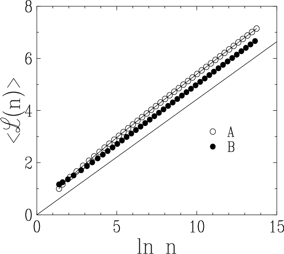
2.2 Number of leads
The number of leads up to time can be estimated by elaborating on the observation [8] that lead changes are driven by the presence of co-leaders. In the present situation, this line of reasoning yields a quantitative result. The probability for a lead change to take place at time is indeed proportional to , the number of co-leaders at time which are not the leader. Furthermore the –st node attaches to each of those co-leaders with probability . We have therefore the exact relation
| (2.9) |
Within the stationary approach, the mean number of co-leaders is shown in Appendix A to have a finite limit (1.29) for large . For we obtain . According to the discussion of Section 2.1, this leading-order result can be trusted to be asymptotically exact for large . Hence
| (2.10) |
Figure 3 shows a plot of against for both initial conditions. The data are observed to follow the logarithmic law (2.10), albeit with appreciable finite-time corrections, especially for Case A.
2.3 Index of the leader
The study of the mean index of the leader at time also follows the line of reasoning of [8]. The essential ingredient is the mean index of a node of degree . This quantity can be derived by the following approach, which does not require any a priori knowledge of asymptotic degree statistics. The mean index of a node of degree at time reads
| (2.11) |
where the denominator has been introduced in (2.4), whereas the numerator,
| (2.12) |
obeys the recursion
| (2.13) |
In the stationary regime ( at fixed ), we have , with
| (2.14) |
hence
| (2.15) |
and finally
| (2.16) |
The mean index of the leader can be estimated by replacing in (2.16) by the logarithmic law (2.7) giving the typical largest degree. We are thus left with [8]
| (2.17) |
The full-fledged stationary approach allows us to derive a better approximation of , including a numerical estimate for the amplitude. Within this framework, averaging the expression (2.16) over the stationary extreme-value statistics of yields , with and , where the generating function is defined in (1.12). The expressions (1.15)–(1.19) corroborate the power law (2.17), and yield the estimate for the amplitude (with ‘stat’ for ‘stationary’).
Figure 4 shows a plot of the ratio against , for both initial conditions. Both series of data seem to converge, albeit very slowly, to a common limit (full line), in the same range as the stationary estimate .

2.4 Lead persistence probability
The lead persistence probability is the probability that the first node keeps the lead up to time . It is suggested in [8] that can be estimated as the probability that the degree of the first node is equal to the mean largest degree, i.e., (see (2.7)), up to negligible finite fluctuation. Elaborating on this line of thought, we propose to give a better derivation of as the probability that the degree of the first node has been equal to the mean largest degree for all times up to the current time . This improvement takes into account the fact that a persistence phenomenon is intrinsically non-local in time.
The distribution of the degree of the first node has been derived in several works. Consider Case A for definiteness. The corresponding generating series reads [8, 11]
| (2.18) |
so that we have
| (2.19) |
In a first step, let us consider the probability for to be very different from its mean value at time (see (2.8)), namely with . This probability can be estimated by applying the saddle-point approximation to the above contour integral. We thus obtain a logarithmic large-deviation estimate of the form
| (2.20) |
with as . The above estimate holds irrespective of the initial condition. In the case of interest, i.e., , the exponent reads [8]. In a second step, we estimate the lead persistence probability as the probability that has been of order for all times up to time , and not only at the current time . The effect of such a condition has been investigated in detail in the case of the one-dimensional lattice random walk [14]. As a general rule, the mere effect is to change the exponent of the ‘prefactor’ from to . We are therefore left with the estimate
| (2.21) |
Figure 5 shows a log-log plot of the lead persistence probability against time , for both initial conditions and up to . The data points are far from being aligned, indicating thus a strong deviation from a pure power law [8]. Moreover, the effective slope over the plotted data range is around 0.3, i.e., four times larger than the theoretical asymptotic exponent (dashed line). The full estimate (2.21) (full line), including the prefactor , gives a much better representation of the data.

2.5 Number of distinct leaders
The mean number of distinct leaders up to time is expected to grow logarithmically:
| (2.22) |
Two heuristic reasons can be given in favor of this law. First, the number of lead changes up to time , , grows much less rapidly than the number of candidates to the lead, which can be estimated as . It is therefore likely that any lead change brings a newcomer to the lead, with some non-zero probability . Second, the growth of the largest degree is modest, so that newcomers have ‘a short way to go’ before they can reach the lead.
Figure 6 shows a plot of the mean number of distinct leaders, against time , for both initial conditions. The picture is somewhat similar to that of Figure 3, with appreciable finite-time corrections, especially for Case A. The data confirm our expectation, namely an asymptotic logarithmic law of the form (2.22), irrespective of the initial condition. The slope of the full line is the outcome of a fit including a correction in . The ratio of to the amplitude of the growth law (2.10) of the mean number of leads yields the probability for any lead change to bring a newcomer to the lead:
| (2.23) |

3 Linear preferential attachment: the Barabási-Albert (BA) model
In the Barabási-Albert (BA) model, node attaches to any earlier node with a probability proportional to the degree of that node. The attachment probability of node to node thus reads
| (3.1) |
where the partition function in the denominator ensures the normalization of the probabilities. It reads (see (1.4)), i.e., , .
3.1 Largest degree
The stationary degree distribution of the BA model can be derived along the lines of Section 2.1. The distribution of the degree of node at time obeys the recursion
| (3.2) |
with for . The distribution of the degree of an arbitrary node therefore obeys the recursion
| (3.3) |
Finally, the stationary degree distribution on an infinite network obeys the recursion
| (3.4) |
hence
| (3.5) |
For a large degree , the stationary distribution and the corresponding cumulative distribution scale as and . Applying the extreme-value argument to the latter estimate, we predict that the largest degree grows as
| (3.6) |
In our quest of the distribution of the largest degree , our first approximation relies on stationary extreme-value statistics. We recall that this approach cannot be exact, for the three reasons exposed in Section 2.1. Within this approach, the distribution of the largest degree can be estimated by means of (1.6). The first term () is clearly leading for large, where is small. We thus obtain a distribution of the form , i.e.,
| (3.7) |
In other words, the ratio
| (3.8) |
is predicted to have a non-trivial asymptotic distribution . Our first approximation to the latter distribution, given by the stationary approach, reads
| (3.9) |
This is the Fréchet distribution known in extreme-value statistics [12]. We have in particular , whereas the second moment is divergent. This feature of the stationary approach is clearly incorrect. Indeed finite-size effects induce a cutoff, beyond which the degree distribution falls off very fast.
Our second approximation consists in incorporating these finite-size effects. This approach is however still inexact, as it complies with point (2) of the discussion of Section 2.1, albeit not with point (3), concerning the dependence of the degree of the node on its index. Finite-size effects on the degree statistics have been investigated in detail in [11]. The distribution of the degree at time and the corresponding cumulative distribution scale as
| (3.10) |
with . Both scaling functions depend on the initial condition. The known exact expressions of [11, Eq. (3.47)] yield
| (3.11) |
Our second approximation to the asymptotic distribution of , given by the stationary approach including finite-size effects, reads therefore
| (3.12) |
(with ‘FSS’ for ‘finite-size scaling’). As expected, this expression is better behaved than the Fréchet distribution (3.9). It falls off as , so that all the moments of are finite. From a quantitative viewpoint, a numerical evaluation of the appropriate integrals yields the estimates and . It is also of interest to get an estimate for the asymptotic value of the reduced variance
| (3.13) |
We obtain similarly and .
Figure 7 shows a plot of the mean rescaled largest degree (left) and of the corresponding reduced variance (right), against , for both initial conditions. Throughout this section on the BA model, simulations are realized by using the redirection algorithm proposed in [15] and recalled in the beginning of Section 4. Data are averaged over different histories up to time . For both quantities shown in the figure, as well as other ones to be presented below, the data nicely converge to asymptotic values which can be measured accurately, with leading corrections proportional to . An explanation for this form of corrections will be given in Section 3.3. The measured asymptotic values read , , and . The estimates for the mean degree are satisfactory: they are only some 10% below the observed values, and correctly predict that is larger than . The approach is however less accurate for the reduced variance, as the estimates are too large at least by some 50%. Figure 8 shows a histogram plot of the distribution of the rescaled largest degree . The large value of time () ensures that the data virtually follow the asymptotic distributions and . Data have been sorted in bins of width , as and .


3.2 Number of leads
The number of leads up to time can again be estimated by considering the effect of co-leaders. The probability of a lead change is still proportional to , whereas each co-leader now has a probability to attach the –st node.
Within the framework of stationary extreme-value statistics, with and , the expression (1.6) shows that the probability of having is small, whereas that of having is still smaller, and so on. In other words, with respect to the UA model, co-leaders are now more rare, but the few ones that are present are more efficient. We thus obtain the estimate
| (3.14) |
For a large time , using the above estimates, the right-hand side can be shown to boil down to . We thus obtain the same logarithmic growth for the mean number of leads as for the UA model [8]:
| (3.15) |
Furthermore the stationary approach yields the estimate for the amplitude.
Figure 9 shows a plot of against for both initial conditions. The data are observed to follow the logarithmic law (3.15), with two different amplitudes, and , in the same range as the estimate of the stationary approach.

3.3 Index of the leader
The essential ingredient is again the mean index of a node of given degree . The numerator of the expression (2.11) can be shown to obey the recursion
| (3.16) |
In the stationary regime, we have again , with
| (3.17) |
hence
| (3.18) |
and finally
| (3.19) |
Replacing in this expression by the power law (3.6) for the typical degree of the leader, we obtain a result of order unity. We are thus led to the conclusion that the index of the leader typically stays finite, and especially that its mean value has a finite limit . Within the framework of stationary extreme-value statistics, evaluating as using (3.7), we obtain the estimate . Finally, as the expression (3.19) admits an expansion in powers of , the stationary approach suggests that the leading finite-time corrections to the limit are proportional to .
Figure 10 shows a plot of the mean index of the leader against , for both initial conditions. The data converge to well-defined asymptotic values and , whereas the leading corrections are observed to be linear in .

3.4 Number of distinct leaders and lead persistence probability
The behavior of these last two quantities can be deduced from what is already known by means of the following line of reasoning. The number of distinct leaders up to time is at most equal to the largest index of the leader up to time , . Loosely speaking, cannot grow typically faster than the index of the leader. It is therefore expected to stay of order unity, and to share with the property of having a finite asymptotic mean . More generally, the whole distribution of the number of distinct leaders is expected to converge to a non-trivial distribution in the limit of long times. Finally, as the lead persistence probability is nothing but the probability that equals one, it is also expected to have a finite limit .
Figure 11 shows a plot of the mean number of distinct leaders (left) and of the persistence probability (right) against , for both initial conditions. The data converge to the asymptotic values , , and . Figure 12 shows a plot of the full distribution of the number of distinct leaders for and both initial conditions. The plotted data are virtually equal to the asymptotic distribution .


4 The general preferential attachment (GPA) model
In the general preferential attachment (GPA) model, the probability of attachment to a node is proportional to the sum of the degree of that node and of a constant parameter , representing the initial attractiveness of a node [9]. This parameter is relevant, as it yields the continuously varying exponents
| (4.1) |
The BA and UA models are respectively recovered when and .
More precisely, in the GPA model the attachment probability of node to node reads
| (4.2) |
The partition function in the denominator reads . It therefore depends on the initial condition according to
| (4.3) |
The stationary degree distribution of the GPA model can be derived along the lines of Section 2.1. The distribution of the degree of node at time obeys the recursion
| (4.4) |
with for . The distribution of the degree of an arbitrary node therefore obeys the recursion
| (4.5) |
Finally, the stationary degree distribution obeys the recursion
| (4.6) |
| (4.7) |
This expression has a power-law decay at large :
| (4.8) |
In the regime where and are both large and comparable, the expression (4.7) assumes the scaling form [11, Eq. (4.29)]:
| (4.9) |
with and
| (4.10) |
The linear behavior as matches the exponential fall-off (2.2) of the UA model, whereas the logarithmic growth as matches the power-law decay (4.8).
The GPA model can be simulated very efficiently (in time ) by means of the following redirection algorithm [15]. At time , in order to attach node , an earlier node is chosen uniformly, and node is attached either to node itself with probability , or to the ancestor of node with probability . The ancestor of is the node to which node has attached at time . The attachment probabilities (4.2) are recovered if the redirection probability is chosen to be equal to the growth exponent (4.1), hence the notation. In particular, the linear attachment probabilities of the BA model are recovered when the redirection probability is . Initial conditions are implemented by requiring that some primordial nodes have no ancestor [15]. For Case A, nodes 1 and 2 have no ancestor, whereas node 1 is the ancestor of node 3. For Case B, node 1 has no ancestor, whereas it is the ancestor of node 2. The numbers of primordial nodes can be read off from the expressions (4.3) of the partition function: these are the integers which appear after the minus signs.
For any finite , i.e., any value of the growth exponent, the GPA model behaves in every respect similarly to the BA model (corresponding to ), investigated in Section 3. The largest degree grows as . Setting , the rescaled variable has a limiting distribution , which depends on and on the initial condition. The mean and the reduced variance converge to finite limits and , with leading corrections proportional to . The mean number of leads scales as , where the amplitude depends on and on the initial condition. Finally, the mean index of the leader, the mean number of distinct leaders, and the lead persistence probability have finite limiting values , and . The leading corrections to these limits are again in . The convergence is therefore very slow at small , where a crossover to the UA model is observed (see below). In practice limiting values cannot be extrapolated from data for reasonable times ( – ) with enough accuracy for .


The dependence of the key asymptotic quantities , , and on the growth exponent for both initial conditions is shown in Figure 13. The data corresponding to the BA model, discussed in Section 3, are recovered for , i.e., right in the middle of the plots. The behavior at both endpoints also deserves some attention.
, i.e., . In this limit, the GPA model boils down to a ballistic growth model. Indeed the attachment probability vanishes for , i.e., the initial degree of each node. As a consequence, with our conventions on the initial states, the first node attracts all the subsequent ones. Its degree grows ballistically as , whereas its lead keeps undisputed. This picture explains the trivial limiting values of the key quantities (, , , ). The leading corrections to these limits are observed to be proportional to , i.e., to .
, i.e., . This regime is more subtle than the previous one. Consider a very large value of the parameter . The scaling behavior (4.9) expresses that the static degree distribution first falls off exponentially, as in the UA model (for ), and then crosses over (for ) to a power-law fall-off with a large exponent (for ). Assume now that the degree under consideration grows as the largest degree in the UA model (see (2.7)). The above crossover then takes place at an exponentially large time , such that becomes comparable to . As a consequence, a rough estimate of the behavior of the key quantities as can be obtained by replacing by in the large-time behavior of the same quantities for the UA model. We have seen in Section 2 that grows as a power law (see (2.17)), whereas falls off as a power law (see (2.21)), and grows logarithmically (see (2.22)). Finally, grows logarithmically, whereas stays finite, hence . We thus obtain the estimates
| (4.11) |
up to multiplicative constants which are not predicted by the crossover argument. In spite of their crudeness, the above estimates are in qualitative agreement with the data shown in Figure 13. The first three quantities indeed exhibit a similar kind of divergence at small , reaching values of order 4 – 6 for . The data for the reduced degree variance are observed to vanish faster than linearly as , and to be compatible with a quadratic law (dashed line). Finally, since the reduced variance vanishes at both endpoints, it has a non-trivial maximum ( and ).
5 Discussion
We have presented a comprehensive study of the statistics of leaders and lead changes in growing networks with preferential attachment. The quantities investigated in this work concern either the leader at a given time (degree and identity of the leader, number of co-leaders) or the whole history of lead changes (number of lead changes, of distinct leaders, lead persistence probability). So far very few works had been devoted to the subject of leaders in this sense, either in growing networks [8, 13] or in other random structures [6, 17]. The present paper is also to some extent a continuation of our previous work [11] on finite-size effects in the degree statistics. Both articles are meant to be systematic and consistent with each other. In particular, the same three different attachment rules (UA, BA, GPA) and the same two different initial conditions (Cases A and B) are dealt with in parallel in both works.
The first and most natural quantity of this area is the largest degree , i.e., the degree of the leader at time . As recalled in the Introduction, there are (at least) three ways of defining a time-dependent characteristic degree scale in a scalefree network (see e.g. [9, 10, 11]):
(i) the cutoff scale , beyond which the stationary degree distribution is strongly affected by finite-size effects;
(ii) the largest degree ;
(iii) the degree of a node with any fixed index, say the first one () for definiteness.
These three degree scales have the same growth law as a function of time , i.e., a logarithmic growth for the UA model, and a power law with exponent in the scalefree case. The agreement between definitions (ii) and (iii) is rather natural, as the first node has the highest chance of being the leader. The agreement between definitions (i) and (ii), although less obvious, can be explained within the framework of what we have called ‘stationary extreme-value statistics’. Although this approach cannot be exact (see Section 2.1), it however turns out to correctly predict the order of magnitude of by the condition that the stationary probability for the degree to be larger than , i.e., the cumulative probability , be of order . This criterion implies that is comparable to , where drops more or less suddenly from large to small values. The above heuristic picture can be complemented with quantitative results. In the UA model, the three degree scales grow logarithmically with time , albeit with different (exactly known) prefactors, and different scalings for fluctuations. The degree of the first node is asymptotically distributed according to a Poissonian law [8, 11, 15] with . The largest degree grows as (see (2.7)), whereas fluctuations around this typical value are of order unity. They are indeed given by a ‘discrete Gumbel law’, studied in Appendix A. Finally, the finite-time cutoff in the degree distribution takes place around , in a narrow range whose width scales as [11]. In the BA model, the above degree scales grow as , whereas fluctuations remain broad, i.e., of order unity in relative value. The degree of the first node is asymptotically distributed according to a geometric law [8, 11, 15] with . The largest degree scales as , where the rescaled variable has a non-trivial limiting distribution , which depends on the initial condition (see Figure 8). This distribution is qualitatively different from the Fréchet distribution predicted by ‘stationary extreme-value statistics’, whereas the Gumbel distribution put forward in [13] cannot be more than a good fit of over some range. Finally, the cutoff scale is also smeared into a non-trivial finite-size scaling law, which also depends on the initial condition (see (3.10)). The same kind of asymptotic results holds more generally for the GPA model, where the growth exponent of the BA model is replaced by the continuously varying exponent .
Our results on the other observables, especially those concerning the whole history of a growing network (number of lead changes, of distinct leaders, lead persistence probability), are the outcome of a blend of heuristic reasoning and accurate numerical work. In the scalefree case (BA and GPA models), the present study confirms and makes more quantitative the picture emerging from the pioneering work of Krapivsky and Redner [8]. The finiteness of and means that a typical infinite history of a scalefree network involves finitely many distinct leaders, which are chosen among the oldest nodes. For the BA model, the numerical results of Section 3, recalled in Table 1, show that the number of distinct leaders is in fact quite small (around two on average), whereas the index of the leader is hardly larger (around three on average). The entire history even consists of a single lead with an appreciable lead persistence probability (around one third). As already underlined in [8], this is a strong form of the rich-get-richer principle.
| Quantity | |||||
| Case A | 2.00 | 0.108 | 3.40 | 2.22 | 0.279 |
| Case B | 2.16 | 0.111 | 2.67 | 1.94 | 0.389 |
| 7 | 3 | 21 | 13 | 28 |
The lead persistence probability and other key quantities exhibit a weak but significative dependence on the initial condition, as demonstrated by the data of Table 1. The feature that scalefree networks remember their whole past forever, and especially their infancy, already visible in finite-size effects on the degree statistics, is thus fully confirmed as a general phenomenon.
Finally, the study of the statistics of leaders and lead changes can be expected to shed some new light onto more complex models. We think especially of the Bianconi-Barabási (BB) model [18], an extension of the BA model where the attachment rule involves both dynamical variables (the node degrees ) and quenched disordered ones (the node fitnesses ). The BB model has the remarkable feature that it may exhibit a continuous transition, somewhat analogous to the Bose-Einstein condensation, or to the condensation transitions which take place in classical stochastic models such as the zero-range process (ZRP) [19]. It is convenient to parametrize the node fitnesses as activated variables: , where the activation energies are drawn from a temperature-independent distribution. The BA model is recovered in the infinite-temperature limit, whereas the opposite zero-temperature limit yields an interesting record-driven growth process, investigated at length in [20]. Depending on the distribution of the , the BB model may have a low-temperature condensed phase below some finite condensation temperature . The dynamics of the model in its condensed phase, already tackled in [21], is not fully understood yet. The statistics of leaders seems to be an appropriate tool, as the condensate should naturally appear as a long lived leader. We intend to return to this problem in a near future.
Appendix A Extreme-value statistics for geometric integer variables
This Appendix gives a self-contained exposition of various results concerning extreme-value statistics for integer variables. The theory of extreme-value statistics is most currently presented in the case of real variables with a continuous distribution [12]. The peculiarities of discrete (e.g. integer) distributions have been underlined in [22].
After some general formalism, we study more extensively the case of a large collection of independent integer variables (), referred to as degrees, drawn from the common geometric distribution
| (1.1) |
The parameter can assume any value in the range . The stationary degree distribution (2.2) of the UA model is recovered for . We consider successively the largest degree, , and the number of co-leaders, i.e., the number of node indices such that .
A1. Distribution of the largest degree
Let us start with some general formalism. The derivation of the distribution of the largest degree follows the usual line of reasoning of extreme-value statistics [12]. Introducing the cumulative distribution
| (1.2) |
so that
| (1.3) |
we have
| (1.4) |
The distribution of the largest degree, , thus reads
| (1.5) |
Using (1.3), this expression can be expanded as
| (1.6) |
The integer is to be interpreted as the number of co-leaders (see (1.25)).
In the present situation of interest, i.e., the geometric distribution (1.1), the above general formulas read
| (1.7) |
and
| (1.8) |
Hereafter we are mostly interested in large values of . In this regime, the latter expression can be ‘exponentiated’ as follows:
| (1.9) |
The mean value of can thus be recast as
| (1.10) |
The sum is dominated by the values of such that is of order unity. We thus obtain the estimate
| (1.11) |
A more refined analysis goes as follows. Consider the generating function
| (1.12) |
The estimate (1.11) suggests to set
| (1.13) |
with integer and for definiteness, and
| (1.14) |
With these notations, the expression (1.12) can be recast as
| (1.15) |
with
| (1.16) |
The amplitude is a periodic function of , with unit period. Its Fourier series can be derived by means of the Poisson summation formula, in the form
| (1.17) |
We thus obtain
| (1.18) |
with
| (1.19) |
The oscillations in the amplitude , described by the Fourier modes with , are extremely small, except if is very close to zero. The Fourier coefficients indeed fall off exponentially as , irrespective of . For , our case of interest, this estimate reads , so that even the first amplitudes () are very small.
Asymptotic expressions for the mean and the variance of the largest degree can be obtained by expanding (1.15) to second order near . Neglecting the tiny periodic oscillations in , i.e., replacing the full function by the constant amplitude , we are left with
| (1.20) |
where denotes Euler’s constant.
It is worth comparing the present problem to its continuous analogue, namely the distribution of , the largest of a large number of i.i.d. random variables , with exponential density , with the identification . This is a standard problem of extreme-value statistics [12]. Setting
| (1.21) |
the reduced variable obeys a Gumbel law with density
| (1.22) |
We have , so that and , hence
| (1.23) |
These results coincide with the first terms of the expressions (1.20), whereas the second terms there, involving rational numbers, are intrinsic effects of discreteness.
We will refer to the distribution (1.9) as a discrete Gumbel law. Let us now turn to other features of this distribution. Using the definitions (1.13), (1.14), the expression (1.9) can be recast as
| (1.24) |
The full distribution exhibits periodic oscillations in , with unit period. These oscillations have been shown to be very small in the case of global characteristics, such as the mean and variance. They are however more visible in the shape of the distribution near its maximum. This shape indeed oscillates between:
(i) a symmetric triangular form
(![[Uncaptioned image]](0911.3057v1/fs.png) )
with a well identified most probable integer,
)
with a well identified most probable integer,
(ii) a flat tabular form
(![[Uncaptioned image]](0911.3057v1/ft.png) )
with two equally probable integers.
)
with two equally probable integers.
This phenomenon is best illustrated by considering the highest probability , i.e., the probability of the most probable integer . This quantity is again a periodic function of , with unit period. It can be checked that the highest probability is reached for (i.e., ) if and for (i.e., ) if , where the threshold value depends on . Situation (ii) corresponds to , where takes its minimal value , the two equally probable integers being and . Situation (i), where takes its maximal value , takes place near . Figure 14 shows a plot of against for . The minimum is reached at the threshold , whereas the maximum is reached for .

A2. Distribution of the number of co-leaders
The distribution of the number of co-leaders can be obtained as follows. The expansion (1.6) allows one to readily write down the joint probability of and as
| (1.25) |
so that the distribution of the number of co-leaders reads
| (1.26) |
Using (1.1), (1.7), the ‘exponentiation’ valid at large , and the definitions (1.13), (1.14), this expression can be recast as
| (1.27) |
The sum again defines a periodic function of , depending on the value of , with unit period. Neglecting tiny periodic oscillations, we are left with the following asymptotic distribution of the number of co-leaders:
| (1.28) |
known as a logarithmic distribution. In particular, the asymptotic mean number of co-leaders reads
| (1.29) |
References
References
- [1] Albert R and Barabási A L, 2002 Rev. Mod. Phys. 74 47
- [2] Dorogovtsev S N and Mendes J F F, 2002 Adv. Phys. 51 1079Dorogovtsev S N and Mendes J F F, 2003 Evolution of Networks (Oxford: Oxford University Press)
- [3] Boccaletti S, Latora V, Moreno Y, Chavez M and Hwang D U, 2006 Phys. Rep. 424 175
- [4] Barrat A, Barthélemy M and Vespignani A, 2008 Dynamical Processes on Complex Networks (Cambridge: Cambridge University Press)
- [5] Barabási A L and Albert R, 1999 Science 286 509Barabási A L, Albert R and Jeong H, 1999 Physica 272 A 173
- [6] Luczak T, 1990 Random Struct. Algorithms 1 287Erdös P and Luczak T, 1994 Random Struct. Algorithms 5 243
- [7] Erdös P and Rényi A, 1959 Publ. Mathematicae 6 290Erdös P and Rényi A, 1960 Publ. Math. Inst. Hungar. Acad. Sci. 5 17
- [8] Krapivsky P L and Redner S, 2002 Phys. Rev. Lett. 89 258703
- [9] Dorogovtsev S N, Mendes J F F and Samukhin A N, 2000 Phys. Rev. Lett. 85 4633
- [10] Boguña M, Pastor-Satorras R and Vespignani A, 2004 Eur. Phys. J. B 38 205
- [11] Godrèche C, Grandclaude H and Luck J M, 2009 J. Stat. Phys. at press [arXiv:0907.1470]
- [12] Gumbel E J, 1958 Statistics of Extremes (New York: Columbia University Press)Galambos J, 1987 The Asymptotic Theory of Extreme Order Statistics (Malabar: Krieger)
- [13] Moreira A A, Andrade J S Jr and Amaral L A N, 2002 Phys. Rev. Lett. 89 268703
- [14] Bauer M, Godrèche C and Luck J M, 1999 J. Stat. Phys. 96 963
- [15] Krapivsky P L and Redner S, 2001 Phys. Rev. E 63 066123Krapivsky P L and Redner S, 2002 J. Phys. A 35 9517
- [16] Krapivsky P L, Redner S and Leyvraz F, 2000 Phys. Rev. Lett. 85 4629
- [17] Ben-Naim E and Krapivsky P L, 2004 Europhys. Lett. 65 151
- [18] Bianconi G and Barabási A L, 2001 Europhys. Lett. 54 436Bianconi G and Barabási A L, 2001 Phys. Rev. Lett. 86 5632
- [19] Spitzer F, 1970 Adv. Math. 5 246Evans M R and Hanney T, 2005 J. Phys. A 38 R195Godrèche C, 2007 Ageing and the Glass Transition (Lecture Notes in Physics 716) (Berlin: Springer) p 261
- [20] Godrèche C and Luck J M, 2008 J. Stat. Mech. P11006
- [21] Ferretti L and Bianconi G, 2008 Phys. Rev. E 78 056102
- [22] Anderson C W, 1970 J. Appl. Prob. 7 99