跳到论文正文
W Papers独立论文阅读器 arXiv:0911.3003 论文正文 计算阅读时间 · 0%
引用这篇论文根据当前论文元数据生成,正式投稿前建议核对。


License: arXiv.org perpetual non-exclusive license
arXiv:0911.3003v1 [math-ph] 16 Nov 2009

The ℤ2\mathbb{Z}_{2} staggered vertex model and its applications

Yacine Ikhlef    Jesper Lykke Jacobsen Affiliation: LPTENS, 24 rue Lhomond, 75231 Paris, France Affiliation: Institut de Physique Théorique, CEA Saclay, 91191 Gif Sur Yvette, France    Hubert Saleur Affiliation: Institut de Physique Théorique, CEA Saclay, 91191 Gif Sur Yvette, France Affiliation: Department of Physics, University of Southern California, Los Angeles, CA 90089-0484    [2.0mm] Section de mathématiques    Université de Genève2-4 rue du Lièvre, CP 64, 1211 Genève 4, Suisse
Abstract

New solvable vertex models can be easily obtained by staggering the spectral parameter in already known ones. This simple construction reveals some surprises: for appropriate values of the staggering, highly non-trivial continuum limits can be obtained. The simplest case of staggering with period two (the ℤ2\mathbb{Z}_{2} case) for the six-vertex model was shown to be related, in one regime of the spectral parameter, to the critical antiferromagnetic Potts model on the square lattice, and has a non-compact continuum limit. Here, we study the other regime: in the very anisotropic limit, it can be viewed as a zig-zag spin chain with spin anisotropy, or as an anyonic chain with a generic (non-integer) number of species. From the Bethe-Ansatz solution, we obtain the central charge c=2c=2, the conformal spectrum, and the continuum partition function, corresponding to one free boson and two Majorana fermions. Finally, we obtain a massive integrable deformation of the model on the lattice. Interestingly, its scattering theory is a massive version of the one for the flow between minimal models. The corresponding field theory is argued to be a complex version of the C2(2)C_{2}^{(2)} Toda theory.

1 Introduction

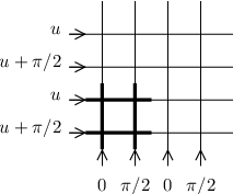
It is a simple consequence of the quantum inverse scattering [1] formalism (going back to Baxter’s ‘Z invariance’ [2]) that new integrable vertex models can be obtained from basic ones by allowing for some staggering of the spectral parameters. If the basic Rˇ\check{R}-matrix is associated with a single crossing , one can in this way build ‘block’ Rˇ\check{R}-matrices, using n2n^{2} crossings, with n=2,3,…n=2,3,\ldots, and staggering the spectral parameters (see Fig. 1).

Refer to caption
Figure 1: The Rˇ\check{R}-matrices for a basic vertex model (left), and for a staggered vertex model with n=2n=2 (right).

While constructing the model and writing down the Bethe equations is straightforward, the physics of the models thus obtained presents interesting subtleties. A striking example was discussed in detail in Refs. [3, 4], in relation with the antiferromagnetic Potts model [5]. It was found then that the case n=2n=2 for the six-vertex model has a non-compact continuum limit [4] in a certain regime of the spectral parameter (see below for a more accurate definition), and may be related to the complex sine-Gordon (SG) model. While major difficulties remain in this case, the other regime of the spectral parameter turns out to be also of interest, and somewhat more tractable. Its study is the main goal of this paper.

Before launching into details, a general discussion about vertex models, spin chains and field theories seems useful. Indeed, the correspondence between integrable spin chains with SU⁡(2){\rm SU}(2) or SU​(2)q{\rm SU}(2)_{q} symmetry and quantum field theories has been investigated in great details already. In the antiferromagnetic regime, it is well known that a chain of spin ss corresponds to a level-2​s2s Weiss-Zumino-Witten (WZW) model in the SU⁡(2){\rm SU}(2) case, and to a deformation of this theory in the Cartan direction for SU​(2)q{\rm SU}(2)_{q} [6]. Cursory examination of the literature would suggest nothing much remains to be done in this area.

From the RR-matrix point of view, models with higher values of the spin ss are obtained by projecting tensor products of (2​s2s) fundamental representations of Uq​(sl2){\rm U}_{q}({\rm sl}_{2}) onto higher spin. This construction has a close parallel in conformal field theory (CFT), where higher level (2​s2s) representations of current algebra are obtained by combining (2​s2s) level one representations. There are several reasons why it would be interesting to build integrable models which are not projected onto irreducible Uq​(sl2){\rm U}_{q}({\rm sl}_{2}) components. In the case s=1s=1 for instance, this would correspond to models of pairs of spin-12\frac{1}{2} variables. This can be reinterpreted more physically in terms of ladders, or, in terms of electron physics, pairs of wires or channels. The latter case is of the highest importance. For instance, the two-channel Kondo model [7] or the two-channel Interacting Resonant Level models [8, 9] are usually solved by going to an even-odd basis, which effectively amounts to solving the problem in the level k=2k=2 sector. Many physical questions are however related to the mixture of the even and odd degrees of freedom – e.g. because it corresponds to transport of electrons between wires. The search for integrable cases where this mixture could be studied is a priority.

To have a better idea of what to expect, it is useful to turn to the CFT point of view. Imagine starting with two SU⁡(2){\rm SU}(2) Kac-Moody algebras at level 1, represented by the currents jiμj_{i}^{\mu}, i=1,2i=1,2 and μ=1,2,3\mu=1,2,3. The sums

Jμ=j1μ+j2μJ^{\mu}=j_{1}^{\mu}+j_{2}^{\mu} (1.1)

are well known to provide then a Kac-Moody algebra at level 2. Of course, each level 1 corresponds to central charge c=1c=1, while level 2 has central charge c=3/2c=3/2. The point is that in taking two copies of level 1, an Ising model CFT factors out, according to the well known-decomposition

SU​(2)1×SU​(2)1=SU2​(2)+ Ising.{\rm SU}(2)_{1}\times{\rm SU}(2)_{1}={\rm SU}_{2}(2)+\hbox{ Ising}\,. (1.2)

This can be illustrated quickly using bosonisation. Introduce two chiral bosons ϕ1,ϕ2\phi_{1},\phi_{2} with propagators

⟨ϕi​(z)​ϕi​(w)⟩=−14​π​ln⁡(z−w).\langle\phi_{i}(z)\phi_{i}(w)\rangle=-\frac{1}{4\pi}\ln(z-w)\,. (1.3)

The two level-1 current algebras are obtained through

ji±∝exp⁡(±i​8​π​ϕi),ji3∝∂ϕi.j_{i}^{\pm}\propto\exp\left(\pm{\rm i}\sqrt{8\pi}\phi_{i}\right)\,,\qquad j_{i}^{3}\propto\partial\phi_{i}\,. (1.4)

It is convenient to introduce now symmetric and antisymmetric combinations of the bosons:

Φ=12​(ϕ1+ϕ2),ϕ=12​(ϕ1−ϕ2).\Phi=\frac{1}{\sqrt{2}}\left(\phi_{1}+\phi_{2}\right)\,,\qquad\phi=\frac{1}{\sqrt{2}}\left(\phi_{1}-\phi_{2}\right)\,. (1.5)

So we have

J±∝cos⁡4​π​ϕ​exp⁡(±i​4​π​Φ),J3∝∂Φ.J^{\pm}\propto\cos\sqrt{4\pi}\phi\ \exp(\pm{\rm i}\sqrt{4\pi}\Phi)\,,\\ \qquad J^{3}\propto\partial\Phi\,. (1.6)

The field cos⁡(4​π​Φ)\cos(\sqrt{4\pi}\Phi) is a Majorana fermion [10]. The field i​sin⁡(4​π​ϕ){\rm i}\sin(\sqrt{4\pi}\phi) is another one, which is orthogonal to the currents JμJ^{\mu}, and is discarded in the construction of SU​(2)2{\rm SU}(2)_{2}. Corresponding to this splitting, the sum H=H1+H2H=H_{1}+H_{2} of the two one-boson Hamiltonians decomposes as H=HSU​(2)2+HIsingH=H_{{\rm SU}(2)_{2}}+H_{\rm Ising} where HSU​(2)2∝∑μ:JμJμ:H_{{\rm SU}(2)_{2}}\propto\sum_{\mu}:J^{\mu}J^{\mu}:, and JμJ^{\mu} are the currents at level two.

Quantum deformations of SU​(2)2{\rm SU}(2)_{2} are obtained by adding to the Hamiltonian HSU​(2)2H_{{\rm SU}(2)_{2}} a Cartan deformation proportional to J3​J3J^{3}J^{3}. We can as well deform the full Hamiltonian, obtaining in this way a theory made of two Majorana fermions and one boson with anisotropy-dependent radius. This should be the continuum limit of the models we are after. We will show in the following that these models are obtained by the general staggering construction, with n=2n=2 and an appropriate choice of the spectral parameters.

Interestingly, it can be shown [11] that the staggered models correspond algebraically to solutions of the Yang-Baxter equations based on ‘bigger’ irreducible representations of the quantum affine algebra Uq​(sl^2){\rm U}_{q}(\widehat{\rm sl}_{2}). This occurs ultimately because finite-dimensional irreducible representations of quantum affine algebras are isomorphic to products of evaluation representations, which are themselves ‘decorations’ (with the spectral parameter) of the usual spin-ss representations of Uq​(sl2){\rm U}_{q}({\rm sl}_{2}) [12].

Another important application of the staggered model is that it can be used to produce a lattice discretisation of a massive QFT. This is done, following Ref. [13], by introducing into the staggered model an additional (purely imaginary) staggering of the spectral parameters. Using this approach, we obtain a scattering theory involving two types of massive particles, where the scattering between particles of the same type (resp. different types) is given by the Sine-Gordon SS-matrix (resp. the Sine-Gordon SS-matrix with an imaginary shift in the rapidity). It turns out that such a scattering theory (but with massless particles) arose before [14] in the context of minimal models of CFT perturbed by the Φ13\Phi_{13} operator. Consider the action:

A=Amin+λ​∫d2​x​Φ13​(x),A=A_{\rm min}+\lambda\int d^{2}x\,\Phi_{13}(x)\,, (1.7)

where AminA_{\rm min} is the action of a minimal model of CFT. The problem of finding the Thermodynamic Bethe Ansatz (TBA) equations for the renormalisation-group flow of the theory (1.7) was first studied by Zamolodchikov in Ref. [15, 16]. The results depend crucially on the sign of the coupling λ\lambda. For λ<0\lambda<0, the model (1.7) becomes massive. It was shown in Ref. [15] that the corresponding SS-matrix is the simple RSOS SS-matrix and that the TBA diagram is of the AnA_{n} type, with a massive particle at one end of the diagram. For λ>0\lambda>0, the model (1.7) describes the massless flow between two consecutive minimal models. In Ref. [16], a TBA diagram was proposed, without resorting to an SS-matrix: this diagram is also of the AnA_{n} type, but with mass terms e±θ{\rm e}^{\pm\theta} at the two ends of the diagram. It was found later, in Ref. [14], that the corresponding scattering theory consists in massless left/right particles, interacting through the SG and shifted-SG SS-matrices.

In summary, we construct here a non-critical lattice model whose continuum excitations are described by a massive version of the SS-matrix for the flow between minimal models of CFT. We also propose an effective QFT for this model, with one boson and two Majorana fermions which interact with each other.

The paper is organised as follows. In Section 2, we expose in more detail the construction of the model and its various lattice formulations, as well as the relation with spin chains and anyonic chains. In Section 3, we present the Bethe-Ansatz solution, and obtain the critical exponents, through the study of low-energy excitations. In Section 4, we discuss the associated CFT, and exhibit the full operator content through the study of torus partition functions. Finally, in Section 5, we study the integrable massive deformation, and derive its scattering theory, TBA equations and ground-state energy scaling function. This allows us to propose an interacting effective QFT. Some important but quite long calculations are done in the Appendices.

2 Solvable Potts models and loop Hamiltonians

In this section, we first recall the definition of the Potts model [17] on the square lattice and its equivalence to a loop model based on the Temperley-Lieb (TL) algebra [18]. Then we introduce a solvable case, involving a staggering of the spectral parameters, and we obtain the expression (2.18) for the associated one-dimensional Hamiltonian, in terms of the TL generators. This solvable model has two critical regimes: regime I corresponds to the antiferromagnetic critical transition [3, 4, 5]; regime II contains a mixture of ferromagnetic and antiferromagnetic couplings, and is the subject of the present paper. Finally, we explain the relation to Majumdar-Ghosh spin chains [19, 20] and anyonic chains [21, 22].

2.1 The Potts model and the Temperley-Lieb algebra

Refer to caption
Figure 2: Equivalence between the cluster and loop models. The full dots represent Potts spins, and the empty dots are the sites of the dual lattice. The thin lines are the edges of the lattice ℒ\cal L. Each cluster configuration corresponds to precisely one loop configuration.

The QQ-state Potts model [17] is a model of classical spins with nearest-neighbour interactions. Each spin SjS_{j} can take QQ values, and sits on a vertex of the square lattice. The Boltzmann weights and the partition function are given by:

W⁡[{Sj}]=∏⟨i​j⟩exp⁡[Ji​j​δ​(Si,Sj)],ZPotts=∑{Sj}W⁡[{Sj}].\begin{array}[]{rcl}W[\{S_{j}\}]&=&{\displaystyle\prod_{\langle ij\rangle}\exp\left[J_{ij}\ \delta(S_{i},S_{j})\right]}\,,\\ Z_{\rm Potts}&=&{\displaystyle\sum_{\{S_{j}\}}W[\{S_{j}\}]}\,.\end{array} (2.1)

where the product runs over all the bonds of the lattice, and the Ji​jJ_{ij} are the coupling constants of the model. This model can be reformulated as a cluster model, called the Fortuin-Kasteleyn model [23], in the following way. We may write the Boltzmann weights as:

W⁡[{Sj}]=∏⟨i​j⟩[1+vi​j​δ​(Si,Sj)],vi​j≡eJi​j−1.W[\{S_{j}\}]=\prod_{\langle ij\rangle}\left[1+v_{ij}\delta(S_{i},S_{j})\right]\,,\qquad v_{ij}\equiv e^{J_{ij}}-1\,. (2.2)

The above expression can be expanded, and each term in the expansion is represented by a subgraph of the square lattice, consisting of the bonds where the δ\delta term has been chosen. When we sum over the spin configurations, the subgraph gets a weight QQ for each of its connected components. So the partition function can be written as:

ZFK=∑GQC⁡(G)​∏⟨i​j⟩∈Gvi​j,Z_{\rm FK}=\sum_{G}Q^{C(G)}\prod_{\langle ij\rangle\in G}v_{ij}\,, (2.3)

where the sum is over all possible subgraphs (or cluster configurations) GG, and C⁡(G)C(G) is the number of connected components of GG. The Fortuin-Kasteleyn model is, in turn, transformed to a dense loop model. Consider the lattice ℒ\cal L obtained by the union of the original square lattice and its dual. Each face of ℒ\cal L contains exactly one Potts bond. By decorating these faces as shown in Fig. 2, we obtain configurations of closed loops on the lattice. The partition function is then:

Zloop=∑GQL⁡(G)/2​∏⟨i​j⟩∈Gvi​jQ,Z_{\rm loop}=\sum_{G}Q^{L(G)/2}\prod_{\langle ij\rangle\in G}\frac{v_{ij}}{\sqrt{Q}}\,, (2.4)

where L⁡(G)L(G) is the number of closed loops.

In the present study, we will restrict ourselves to the case when the couplings are Ji​j=J1J_{ij}=J_{1} on horizontal bonds and Ji​j=J2J_{ij}=J_{2} on vertical bonds. Then, for the loops, a plaquette can be of two types, according to the direction of the Potts bond it contains. The local Boltzmann weights for the loop plaquettes can be written:

[Uncaptioned image] (2.5)

where x⁡(u)=v1/Qx(u)=v_{1}/\sqrt{Q} for plaquettes of type 1 and x⁡(u)=Q/v2x(u)=\sqrt{Q}/v_{2} for plaquettes of type 2. The non-local weights for closed loops are encoded in the Temperley-Lieb algebra [18], with generators (ej)j=1​…​2​N(e_{j})_{j=1\dots 2N}:

ej2=Q​ejej​ej±1​ej=ejej​ej′=ej′​ejif |j−j′|>1.\begin{array}[]{l}e_{j}^{2}=\sqrt{Q}\ e_{j}\\ e_{j}e_{j\pm 1}e_{j}=e_{j}\\ e_{j}e_{j^{\prime}}=e_{j^{\prime}}e_{j}\qquad\text{if $|j-j^{\prime}|>1$}\,.\end{array} (2.6)

These relations are interpreted graphically as follows: jj is the site index in the horizontal direction, and eje_{j} is the represented by the second term of Eq. (2.5) at position jj (see Fig. 3). The loop weight Q\sqrt{Q} is parameterised as:

Q=2​cos⁡γ,0≤γ≤π2.\sqrt{Q}=2\cos\gamma\,,\qquad 0\leq\gamma\leq\frac{\pi}{2}\,. (2.7)
Refer to caption
Figure 3: The Temperley-Lieb algebraic relations (2.6).

2.2 Solvable inhomogeneous Potts model

To construct a solvable model, the first step is to obtain an Rˇ\check{R}-matrix which satisfies the Yang-Baxter equations:

Rˇj,j+1​(u)​Rˇj+1,j+2​(u−v)​Rˇj,j+1​(v)=Rˇj+1,j+2​(v)​Rˇj,j+1​(u−v)​Rˇj+1,j+2​(u).\check{R}_{j,j+1}(u)\check{R}_{j+1,j+2}(u-v)\check{R}_{j,j+1}(v)=\check{R}_{j+1,j+2}(v)\check{R}_{j,j+1}(u-v)\check{R}_{j+1,j+2}(u)\,. (2.8)

The Temperley-Lieb algebra (2.6) provides a solution to these equations:

Rˇj,j+1​(u)≡sin⁡(γ−u)​ 1+sin⁡u​ej.\check{R}_{j,j+1}(u)\equiv\sin(\gamma-u)\ 1+\sin u\ e_{j}\,. (2.9)

Comparing with (2.5), the local weight xx is given by:

x⁡(u)=sin⁡usin⁡(γ−u).x(u)=\frac{\sin u}{\sin(\gamma-u)}\,. (2.10)

Using this Rˇ\check{R}-matrix, we can construct a solvable model on the square lattice, by choosing the spectral parameters along the lines of the lattice. Suppose, from now on, that the square lattice where the loops live consists of horizontal and vertical lines. To respect the alternation J1,J2J_{1},J_{2} of the Potts coupling constants, we have to use the spectral parameters (u,u+α,u,u+α,…)(u,u+\alpha,u,u+\alpha,\dots) and (0,α,0,α,…)(0,\alpha,0,\alpha,\dots), and also ensure that Rˇ​(u+α)∝Rˇ​(u−α)\check{R}(u+\alpha)\propto\check{R}(u-\alpha). This holds only for α=0\alpha=0 or α=π/2\alpha=\pi/2.

Refer to caption
Figure 4: The Yang-Baxter equations (2.8).

The case α=0\alpha=0 is the homogeneous TL loop model, and corresponds to the well-studied self-dual Potts model. It has two critical regimes: 0<u<γ0<u<\gamma is the ferromagnetic critical transition, and γ<u<π\gamma<u<\pi is the ‘non-physical self-dual line’, governing the critical Berker-Kadanoff phase [32].

In the present paper, we are interested in the case α=π/2\alpha=\pi/2, which we call the ℤ2\mathbb{Z}_{2} staggered model. The parameters v1,v2v_{1},v_{2} are then given by:

v1Q=sin⁡usin⁡(γ−u),v2Q=−cos⁡(γ−u)cos⁡u.\frac{v_{1}}{\sqrt{Q}}=\frac{\sin u}{\sin(\gamma-u)}\,,\qquad\frac{v_{2}}{\sqrt{Q}}=-\frac{\cos(\gamma-u)}{\cos u}\,. (2.11)

There are again two regimes:

  • •

    Regime I: γ<u<π/2\gamma<u<\pi/2.
    In this regime, we have v1<0v_{1}<0 and v2<0v_{2}<0. This was identified by Baxter [5] as the location of the antiferromagnetic critical transition. There is an isotropic point u=π2+γ2u=\frac{\pi}{2}+\frac{\gamma}{2} for which v1=v2v_{1}=v_{2}. The exact solution on the lattice, and the corresponding field theory were studied in detail previously [3, 4].

  • •

    Regime II: 0<u<γ0<u<\gamma.
    In this regime, we have now v1>0v_{1}>0 and v2<0v_{2}<0. There is thus no isotropic point, but for u=γ2u=\frac{\gamma}{2} we have that v1=−v2v_{1}=-v_{2} differ only by a sign; we shall see that at this point isotropy is recovered in the continuum limit. In the following, we will focus our attention on this regime.

Let us now recall the lattice structure of the staggered model [3, 4]. This is better described by the block ℛˇ\check{\cal R}-matrix (see Fig. 5):

ℛˇj,j+1​(u)≡Rˇ2​j,2​j+1​(u−π/2)​Rˇ2​j−1,2​j​(u)​Rˇ2​j+1,2​j+2​(u)​Rˇ2​j,2​j+1​(u+π/2).\check{\cal R}_{j,j+1}(u)\equiv\check{R}_{2j,2j+1}(u-\pi/2)\check{R}_{2j-1,2j}(u)\check{R}_{2j+1,2j+2}(u)\check{R}_{2j,2j+1}(u+\pi/2)\,. (2.12)

Using (2.9), we get the expression for ℛˇj,j+1​(u)\check{\cal R}_{j,j+1}(u) in terms of the TL generators eje_{j}:

ℛˇj,j+1​(u)\displaystyle\check{\cal R}_{j,j+1}(u) =\displaystyle= −14​sin2⁡(2​γ−2​u)​ 1−12​sin⁡u​sin⁡(2​γ−2​u)​[cos⁡(γ−u)​(e2​j−1+e2​j+1)+2​cos⁡γ​cos⁡u​e2​j]\displaystyle-\frac{1}{4}\sin^{2}(2\gamma-2u)\ 1-\frac{1}{2}\sin u\sin(2\gamma-2u)\left[\cos(\gamma-u)(e_{2j-1}+e_{2j+1})+2\cos\gamma\cos u\ e_{2j}\right] (2.13)
+14​sin⁡2​u​sin⁡(2​γ−2​u)​(e2​j−1​e2​j+e2​j​e2​j−1+e2​j​e2​j+1+e2​j+1​e2​j)\displaystyle+\frac{1}{4}\sin 2u\sin(2\gamma-2u)\ (e_{2j-1}e_{2j}+e_{2j}e_{2j-1}+e_{2j}e_{2j+1}+e_{2j+1}e_{2j})
+sin2⁡u​cos⁡u⁡[cos⁡(γ−u)​(e2​j−1​e2​j+1​e2​j+e2​j​e2​j−1​e2​j+1)−cos⁡u​e2​j​e2​j−1​e2​j+1​e2​j].\displaystyle+\sin^{2}u\cos u\left[\cos(\gamma-u)\ (e_{2j-1}e_{2j+1}e_{2j}+e_{2j}e_{2j-1}e_{2j+1})-\cos u\ e_{2j}e_{2j-1}e_{2j+1}e_{2j}\right]\,.

As a consequence of the Yang-Baxter equations, ℛˇj,j+1​(u)\check{\cal R}_{j,j+1}(u) commutes with the operator:

cj≡(cos⁡γ)−2​Rˇ2​j−1,2​j​(π/2)​Rˇ2​j+1,2​j+2​(π/2).c_{j}\equiv(\cos\gamma)^{-2}\ \check{R}_{2j-1,2j}(\pi/2)\check{R}_{2j+1,2j+2}(\pi/2)\,. (2.14)

Furthermore, using the TL algebraic relations, we see that cj2=1c_{j}^{2}=1. Thus, the ℛˇ\check{\cal R}-matrix has a ℤ/2​ℤ\mathbb{Z}/2\mathbb{Z} symmetry, arising from the staggered structure. We call t⁡(u)t(u) the one-row transfer matrix, with horizontal spectral parameter uu and vertical spectral parameters (0,π/2,0,π/2,…)(0,\pi/2,0,\pi/2,\dots). We consider a lattice of width 2​N2N sites and height 2​M2M sites. The partition function of the staggered model with periodic boundary conditions is then:

ZM​N=Tr​[t⁡(u)​t​(u+π/2)]M.Z_{MN}={\rm Tr}\ \left[t(u)t(u+\pi/2)\right]^{M}\,. (2.15)

The two-row transfer-matrix t⁡(u)​t​(u+π/2)t(u)t(u+\pi/2) commutes with the ℤ/2​ℤ\mathbb{Z}/2\mathbb{Z} ‘charge operator’:

C≡∏j=1N[(cos⁡γ)−1​Rˇ2​j−1,2​j​(π/2)].C\equiv\prod_{j=1}^{N}\left[(\cos\gamma)^{-1}\ \check{R}_{2j-1,2j}(\pi/2)\right]\,. (2.16)
Refer to caption
Figure 5: Lines of spectral parameters for the staggered model. The block ℛˇ\check{\cal R}-matrix is represented in bold lines.

2.3 Very anisotropic limit

An interesting aspect of Yang-Baxter integrable statistical models is that the transfer matrix generally possesses a very anisotropic limit, where its derivatives with respect to uu are local, one-dimensional Hamiltonians. In the expression (2.13) for the block ℛˇ\check{\cal R}-matrix, we observe that ℛˇj,j+1​(0)=−14​sin2⁡2​γ​ 1\check{\cal R}_{j,j+1}(0)=-\frac{1}{4}\sin^{2}2\gamma\ 1, and so the two-row transfer-matrix reduces to a cyclic translation of two sites to the right in the limit u→0u\to 0. The first-order Hamiltonian is:

H≡−12sin2γd​log⁡[t⁡(u)​t​(u+π/2)]d​u|u=0=−12sin2γ∑j=1Nℛˇj,j+1(0)−1d​ℛˇj,j+1d​u(0),H\equiv-\frac{1}{2}\sin 2\gamma\ \left.\frac{{\rm d}\log[t(u)t(u+\pi/2)]}{{\rm d}u}\right|_{u=0}=-\frac{1}{2}\sin 2\gamma\ \sum_{j=1}^{N}\check{\cal R}_{j,j+1}(0)^{-1}\frac{{\rm d}\check{\cal R}_{j,j+1}}{{\rm d}u}(0)\,, (2.17)

which gives:

H=2​N​cos⁡2​γ​ 1+∑j=12​N(−2​cos⁡γ​ej+ej​ej+1+ej+1​ej).H=2N\cos 2\gamma\ 1+\sum_{j=1}^{2N}\left(-2\cos\gamma\ e_{j}+e_{j}e_{j+1}+e_{j+1}e_{j}\right)\,. (2.18)

For a generic value of γ\gamma, the TL algebra can be represented as acting on a chain of spin-12\frac{1}{2} variables with Uq​(sl2){\rm U}_{q}({\rm sl}_{2}) symmetry (for q=ei​γq={\rm e}^{{\rm i}\gamma}). Indeed, consider the Hilbert space [span⁡(|↑⟩,|↓⟩)]⊗2​N[{\rm span}(|\uparrow\rangle,|\downarrow\rangle)]^{\otimes 2N}, describing 2​N2N spins (σ1,…,σ2​N)(\sigma_{1},\dots,\sigma_{2N}), and take two consecutive spins σj,σj+1\sigma_{j},\sigma_{j+1}: the total spin σj+σj+1\sigma_{j}+\sigma_{j+1} can be in the representation of spin 00 or 11. We call Pj,j+1(0)P^{(0)}_{j,j+1} the projector onto spin-00 according to this decomposition. Then it turns out that the unnormalised projectors

ej≡2​cos⁡γ​Pj,j+1(0)e_{j}\equiv 2\cos\gamma\ P^{(0)}_{j,j+1} (2.19)

satisfy the TL algebra (2.6). In terms of the Pauli matrices, the generators (2.19) can be written:

ej=−(σj+​σj+1−+σj−​σj+1+)+12​(1−σjz​σj+1z)​ei​γ​σj+1z.e_{j}=-(\sigma_{j}^{+}\sigma_{j+1}^{-}+\sigma_{j}^{-}\sigma_{j+1}^{+})+\frac{1}{2}(1-\sigma_{j}^{z}\sigma_{j+1}^{z}){\rm e}^{{\rm i}\gamma\sigma_{j+1}^{z}}\,. (2.20)

Using this representation, the first summand in (2.18) would simply give the XXZ spin chain. The quadratic terms in ej,ej+1e_{j},e_{j+1} are due to the staggering, and lead to a different spin model. After some algebra with the Pauli matrices, we obtain:

ej​ej+1+ej+1​ej\displaystyle e_{j}e_{j+1}+e_{j+1}e_{j} =\displaystyle= 12+(σj+​σj+2−+σj−​σj+2+)+12​σjz​σj+2z\displaystyle\frac{1}{2}+(\sigma_{j}^{+}\sigma_{j+2}^{-}+\sigma_{j}^{-}\sigma_{j+2}^{+})+\frac{1}{2}\sigma_{j}^{z}\sigma_{j+2}^{z} (2.21)
−ei​γ​σj+2z​(σj+​σj+1−+σj−​σj+1+)−12​σjz​σj+1z\displaystyle-{\rm e}^{{\rm i}\gamma\sigma_{j+2}^{z}}(\sigma_{j}^{+}\sigma_{j+1}^{-}+\sigma_{j}^{-}\sigma_{j+1}^{+})-\frac{1}{2}\sigma_{j}^{z}\sigma_{j+1}^{z}
−e−i​γ​σjz​(σj+1+​σj+2−+σj+1−​σj+2+)−12​σj+1z​σj+2z.\displaystyle-{\rm e}^{-{\rm i}\gamma\sigma_{j}^{z}}(\sigma_{j+1}^{+}\sigma_{j+2}^{-}+\sigma_{j+1}^{-}\sigma_{j+2}^{+})-\frac{1}{2}\sigma_{j+1}^{z}\sigma_{j+2}^{z}\,.

Let us write our quadratic TL Hamiltonian (2.18) more generally as:

H⁡(K1,K2)=K1​∑j=12​Nej+K2​∑j=12​N(ej​ej+1+ej+1​ej).H(K_{1},K_{2})=K_{1}\sum_{j=1}^{2N}e_{j}+K_{2}\sum_{j=1}^{2N}(e_{j}e_{j+1}+e_{j+1}e_{j})\,. (2.22)

Then, from (2.20)-(2.21), the above Hamiltonian can be written:

H⁡(K1,K2)=∑j=12​N{J22​𝝈j⋅𝝈j+2+J1x​y​(σj+​σj+1−+σj−​σj+1+)+J1z​σjz​σj+1z+i​J3​(σj−1z−σj+2z)​(σj+​σj+1−+σj−​σj+1+)},H(K_{1},K_{2})=\sum_{j=1}^{2N}\left\{\frac{J_{2}}{2}\boldsymbol{\sigma}_{j}\cdot\boldsymbol{\sigma}_{j+2}+J_{1}^{xy}(\sigma_{j}^{+}\sigma_{j+1}^{-}+\sigma_{j}^{-}\sigma_{j+1}^{+})+J_{1}^{z}\sigma_{j}^{z}\sigma_{j+1}^{z}+{\rm i}J_{3}(\sigma_{j-1}^{z}-\sigma_{j+2}^{z})(\sigma_{j}^{+}\sigma_{j+1}^{-}+\sigma_{j}^{-}\sigma_{j+1}^{+})\right\}\,, (2.23)

where:

J1x​y=−(K1+2​cos⁡γ​K2),J1z=−(12​cos⁡γ​K1+K2),J2=K2,J3=K2​sin⁡γ.J_{1}^{xy}=-(K_{1}+2\cos\gamma\,K_{2})\,,\quad J_{1}^{z}=-\left(\frac{1}{2}\cos\gamma\,K_{1}+K_{2}\right)\,,\qquad J_{2}=K_{2}\,,\qquad J_{3}=K_{2}\sin\gamma\,. (2.24)

The J2J_{2} term in equation (2.23) represents two XXX spin chains, living on the even and odd sites respectively. The J1J_{1} terms correspond to an XXZ interaction with a ‘zig-zag’ shape (see Fig. 6). The J3J_{3} term is an anti-Hermitian three-spin interaction, with no obvious physical interpretation.

In the case of our ℤ2\mathbb{Z}_{2} staggered model, we have (K1,K2)=(−2​cos⁡γ,1)(K_{1},K_{2})=(-2\cos\gamma,1), and so J2=1,J1x​y=0,J1z=−sin2⁡γJ_{2}=1,J_{1}^{xy}=0,J_{1}^{z}=-\sin^{2}\gamma. Thus the Hermitian terms of (2.23) correspond to two antiferromagnetic XXX spin chains with a ferromagnetic −σz​σz-\sigma^{z}\sigma^{z} zig-zag interaction. Let us discuss the consequences of a naive bosonisation [24] argument for this model. We can discard the irrelevant J3J_{3} term, and we end up with two free bosons ϕ1,ϕ2\phi_{1},\phi_{2} with compactification radii R1=R2=RR_{1}=R_{2}=R independent from γ\gamma, coupled by the quadratic term J1z​∂ϕ1​∂ϕ2J_{1}^{z}\partial\phi_{1}\partial\phi_{2}. Since this term is symmetric in the exchange of the bosons (ϕ1↔ϕ2\phi_{1}\leftrightarrow\phi_{2}), the symmetric and antisymmetric combinations Φ=(ϕ1+ϕ2)/2,ϕ=(ϕ1−ϕ2)/2\Phi=(\phi_{1}+\phi_{2})/\sqrt{2},\phi=(\phi_{1}-\phi_{2})/\sqrt{2} are decoupled free bosons, with compactification radii R±=R±δ​RR_{\pm}=R\pm\delta R, where δ​R\delta R depends on γ\gamma through J1zJ_{1}^{z}. Thus, we obtain two decoupled free bosons Φ,ϕ\Phi,\phi with both radii depending on γ\gamma. However, using the Bethe Ansatz exact solution of the staggered model (see Section 3), we find that the continuum limit consists of two free bosons with one radius depending on γ\gamma, and the other radius independent of γ\gamma. It seems then that the bosonisation approach misses an important effect due to the anti-Hermitian J3J_{3} term in (2.23).

Refer to caption
Figure 6: Zig-zag spin chain with J1J_{1} and J2J_{2} interactions.

Let us go back to the model (2.22) with general values of K1,K2K_{1},K_{2}, which was studied numerically in Ref. [25]. Additionally to the ℤ2\mathbb{Z}_{2} staggered integrable model, this Hamiltonian contains a remarkable point at (K1,K2)=(−4​cos⁡γ,1)(K_{1},K_{2})=(-4\cos\gamma,1). This was identified in Ref. [20] as the qq-deformed version of the Majumdar-Ghosh (MG) spin chain [19]. The latter was defined as an SU⁡(2){\rm SU}(2) spin-12\frac{1}{2} chain with nearest- and next-nearest-neighbour interactions, for which the totally dimerised state (where the pairs of spins σ2​j−1,σ2​j\sigma_{2j-1},\sigma_{2j} form a singlet) is the exact ground state. The excitations of the isotropic MG chain are known to be gapped spinons [26]. In Ref. [25] it was proved that for γ=π/t\gamma=\pi/t with t≥5t\geq 5 integer, the dimerised state is still a ground state, and numerical evidence was given for the existence of a gapped MG phase in the model (2.22) for generic γ\gamma in the range (n∗≃1.5)<2​cos⁡γ<2(n^{*}\simeq 1.5)<2\cos\gamma<2.

2.4 Relation to anyonic chains

We end this Section by mentioning an additional motivation for the study of TL Hamiltonians such as (2.22), which is their connection to ‘anyonic chains’, an object introduced and studied recently [21, 22]. The starting point is the Read-Rezayi construction [27] of trial wavefunctions for the Fractional Quantum Hall Effect. Following this approach, the trial wavefunctions are given by the correlation functions of the ℤk\mathbb{Z}_{k} parafermionic CFTs. The elementary excitations above the ground state (anyons) then obey the fusion rules given by these CFTs.

The anyonic chain, defined in Ref. [21] for the ℤ3\mathbb{Z}_{3} parafermionic CFT, consists of M+2M+2 anyons with short-range interaction. Each anyon lives in a Hilbert space whose basis elements are labelled by the primary fields of the CFT. In the case of the ℤ3\mathbb{Z}_{3} parafermionic CFT, the primary fields are 11 and τ\tau, with the fusion rule:

τ×τ=1+τ.\tau\times\tau=1+\tau\,. (2.25)

We fix M+2M+2 anyons along a chain to be in the non-trivial state τ\tau, and give an interaction energy to the different ways they can fuse with one another. Suppose the τ\tau-anyons are allowed to fuse according to the linear diagram shown in Fig. 7a, where the xjx_{j} are also anyons. Locally, the fusion diagram between two consecutive τ\tau-anyons and the anyons xj−1,xj+1x_{j-1},x_{j+1} can be rewritten in terms of a new anyonic variable x~j\widetilde{x}_{j}, using the FF-matrix (see Fig. 7b). The variable x~j\widetilde{x}_{j} now results from the direct fusion of the two consecutive τ\tau-anyons. We give energy −ϵ-\epsilon to the configuration x~j=1\widetilde{x}_{j}=1, and energy 00 to the configuration x~j=τ\widetilde{x}_{j}=\tau. Let us describe the Hilbert space and the interaction Hamiltonian in terms of the intermediary states xjx_{j}. The basis of the Hilbert space is labelled by the words x1​…​xM−1x_{1}\dots x_{M-1} on the alphabet {1,τ}\{1,\tau\} which are allowed by the fusion rules. These are the words which do not have the word 1111 as a subword. Fig. 7b defines a local change of basis |xj⟩→|x~j⟩|x_{j}\rangle\to|\widetilde{x}_{j}\rangle. In this new basis, the interaction term defined above is proportional to the projector p~j=|1⟩​⟨1|\widetilde{p}_{j}=|1\rangle\langle 1|. Transforming back to the xjx_{j} basis, we get the operators pjp_{j}, given by ⟨x′|pj|x⟩=(Fτ​xj+1τ​xj−1)x′​1​(Fτ​xj+1τ​xj−1)1​x\langle x^{\prime}|p_{j}|x\rangle=(F^{\tau x_{j-1}}_{\tau x_{j+1}})_{x^{\prime}1}(F^{\tau x_{j-1}}_{\tau x_{j+1}})_{1x}. The total Hamiltonian is then defined as

Hanyons=−ϵ∑j=0M−1pj.H_{\rm anyons}=-\epsilon\ \sum_{j=0}^{M-1}p_{j}\,. (2.26)
Refer to caption
Figure 7: (a) Anyonic chain. (b) Transformation of fusion diagrams through the FF-matrix. Figures reproduced from Ref. [21].

We are now ready to state the correspondence between the anyonic chain and our Hamiltonian HH (2.18). The expression of the FF-matrix is such that the unnormalised projectors ej=(2​cos⁡π5)​pje_{j}=(2\cos\frac{\pi}{5})\,p_{j} satisfy the TL algebra (2.6) for Q=2​cos⁡π5\sqrt{Q}=2\cos\frac{\pi}{5} [21]. In fact, the allowed words x1​…​xM−1x_{1}\dots x_{M-1} are in bijection with the A4A_{4} RSOS configurations, and the operators eje_{j} act on them as in the A4A_{4} RSOS model. This exact correspondence holds in general between the ℤk\mathbb{Z}_{k} anyonic chain and the Ak+1A_{k+1} RSOS model, with the loop weight Q=2​cos⁡πk+2\sqrt{Q}=2\cos\frac{\pi}{k+2}.

Let us recall briefly the construction of the RSOS representation of the TL algebra [28], in the case of the ApA_{p} models. The basis states for the vector space ℋ\cal H are labelled by M=2​NM=2N height variables (h1,…,h2​N)(h_{1},\dots,h_{2N}), such that, for all jj:

hj∈{1,…,p},|hj−hj+1|=1.h_{j}\in\{1,\dots,p\}\,,\qquad|h_{j}-h_{j+1}|=1\,. (2.27)

Then we define the operators (ej)j=1​…​2​N(e_{j})_{j=1\dots 2N} acting on ℋ\cal H by their action on the basis states:

ej​|h1​…​h2​N⟩\displaystyle e_{j}|h_{1}\dots h_{2N}\rangle =\displaystyle= δhj−1,hj+1​∑|hj′−hj+1|=1S⁡(hj)​S​(hj′)S⁡(hj+1)​|h1​…​hj′​…​h2​N⟩,\displaystyle\delta_{h_{j-1},h_{j+1}}\sum_{|h^{\prime}_{j}-h_{j+1}|=1}\frac{\sqrt{S(h_{j})S(h^{\prime}_{j})}}{S(h_{j+1})}|h_{1}\dots h^{\prime}_{j}\dots h_{2N}\rangle\,, (2.28)
S⁡(h)\displaystyle S(h) =\displaystyle= sin⁡π​hp+1.\displaystyle\sin\frac{\pi h}{p+1}\,. (2.29)

It can be shown [28] that these operators satisfy the TL algebra (2.6) with loop weight Q=2​cos⁡π/(p+1)\sqrt{Q}=2\cos\pi/(p+1). In the particular case of ℤ3\mathbb{Z}_{3} anyons, the bijection xj→hjx_{j}\to h_{j} reads:

1→1,τ→3\displaystyle 1\to 1\,,\ \tau\to 3 for jj odd
1→4,τ→2\displaystyle 1\to 4\,,\ \tau\to 2 for jj even

Note that this maps the anyonic words x1​…​xM−1x_{1}\dots x_{M-1} to the subset of RSOS configurations such that even sites jj carry even heights hjh_{j}. However, this subset and its complementary (where even sites carry odd heights) are not coupled by the eje_{j}. The two sectors are related by a one-site translation. Hence the equivalence between ℤ3\mathbb{Z}_{3} anyons and A4A_{4} RSOS is valid up to a degeneracy factor of two.

From this equivalence between anyonic chains and RSOS models, one understands that HanyonsH_{\rm anyons} (2.26) is just an RSOS version of the well-studied XXZ model with anisotropy Δ=Q/2\Delta=\sqrt{Q}/2. It is known [29] that the corresponding effective field theories are the CFT minimal models. More interestingly, in Ref. [22], a three-site interaction was introduced:

Hanyons′=α​∑j=0M−1pj+β​∑j=1Mpj′,H^{\prime}_{\rm anyons}=\alpha\sum_{j=0}^{M-1}p_{j}+\beta\sum_{j=1}^{M}p^{\prime}_{j}\,, (2.30)

where pj′p^{\prime}_{j} denotes the projector onto the 11-channel for the fusion of the τ\tau-anyons at positions (j,j+1,j+2)(j,j+1,j+2). Hamiltonian Hanyons′H^{\prime}_{\rm anyons} is the RSOS representation of the quadratic TL Hamiltonian (2.22). In the context of anyons, only Beraha values Q=2​cos⁡π/(p+1)\sqrt{Q}=2\cos\pi/(p+1) with p=3,4,5,…p=3,4,5,\ldots are allowed, whereas the loop formulation exists for generic QQ. Hence H⁡(K1,K2)H(K_{1},K_{2}) (2.22) is really a generalisation of Hanyons′H^{\prime}_{\rm anyons} (2.30). Numerical studies [22, 25] have shown that the phase diagram of this model is very rich. In particular, it contains a critical phase renormalising to the XXZ Hamiltonian, a gapped phase of MG type (see above), and another critical phase governed by the integrable ℤ2\mathbb{Z}_{2} model which is studied in the present paper. It was also shown in these works that the transition between the XXZ and MG phase is in the universality class of the dilute O⁡(n){\rm O}(n) model, with n=Qn=\sqrt{Q}. We recall the results of [25] in Fig. 8, where we have used the same conventions as in [22] to parameterise the interaction:

K1=2​Q​sin⁡θ−cos⁡θK2=−sin⁡θ.\begin{array}[]{rcl}K_{1}&=&2\sqrt{Q}\ \sin\theta-\cos\theta\\ K_{2}&=&-\sin\theta\,.\end{array} (2.31)

The phase diagram is represented in the range [θℤ2,0][\theta_{\mathbb{Z}_{2}},0], where θℤ2=ArctanQ−1/2−π\theta_{\mathbb{Z}_{2}}={\rm Arctan\ Q^{-1/2}}-\pi is the value corresponding to the ℤ2\mathbb{Z}_{2} model.

Refer to caption
Figure 8: Phase diagram of the quadratic Temperley-Lieb Hamiltonian (2.22), using the parameterisation (2.31). The shaded area is the gapped phase, governed by the MG line (dotted line). Full lines represent phase transitions from the MG phase to the XXZ critical phase (bottom) and the ℤ2\mathbb{Z}_{2} critical phase (top). The ℤ2\mathbb{Z}_{2} staggered model sits on the topmost horizontal line θ=θℤ2\theta=\theta_{\mathbb{Z}_{2}}.

3 Bethe Ansatz solution

In this section, we present the solution by Bethe Ansatz of the model presented in Section 2. We find that the Bethe roots form two coupled Fermi seas, and the elementary excitations are holes close to the Fermi levels. In the continuum limit, we obtain the dressed momentum and energy (3.21) of the holes, and the dressed scattering amplitudes (3.26) between them. The central charge of the theory is c=2c=2. Using the Wiener-Hopf technique for the computation of finite-size corrections (see Appendix B), we derive the conformal spectrum (3.30). It has the form of a two-component Coulomb gas.

3.1 Bethe Ansatz Equations

We use the Algebraic Bethe Ansatz [1], and we define the Bethe roots αj\alpha_{j} as: αj=i⁡(γ−2​uj)\alpha_{j}={\rm i}(\gamma-2u_{j}). The Bethe Ansatz Equations (BAE) and the eigenvalues and eigenvectors of the transfer matrix t⁡(u)t(u) in the rr-particle sector are:

[sinh⁡(αj−i​γ)sinh⁡(αj+i​γ)]N=−e2​i​ϕ∏l=1rsinh⁡12​(αj−αl−2​i​γ)sinh⁡12​(αj−αl+2​i​γ),\left[\frac{\sinh(\alpha_{j}-{\rm i}\gamma)}{\sinh(\alpha_{j}+{\rm i}\gamma)}\right]^{N}=-{\rm e}^{2{\rm i}\phi}\prod_{l=1}^{r}\frac{\sinh\frac{1}{2}(\alpha_{j}-\alpha_{l}-2{\rm i}\gamma)}{\sinh\frac{1}{2}(\alpha_{j}-\alpha_{l}+2{\rm i}\gamma)}\,, (3.1)
Λ⁡(u)=12N​{ei​ϕ​[sin⁡2​(γ−u)]N​∏j=1rsinh⁡12​[i​γ+(αj+2​i​u)]sinh⁡12​[i​γ−(αj+2​i​u)]+e−i​ϕ​(−sin⁡2​u)N​∏j=1rsinh⁡12​[i​γ−(αj+2​i​u−2​i​γ)]sinh⁡12​[i​γ+(αj+2​i​u−2​i​γ)]},\Lambda(u)=\frac{1}{2^{N}}\left\{{\rm e}^{{\rm i}\phi}[\sin 2(\gamma-u)]^{N}\prod_{j=1}^{r}\frac{\sinh\frac{1}{2}\left[{\rm i}\gamma+(\alpha_{j}+2{\rm i}u)\right]}{\sinh\frac{1}{2}\left[{\rm i}\gamma-(\alpha_{j}+2{\rm i}u)\right]}+\ {\rm e}^{-{\rm i}\phi}(-\sin 2u)^{N}\prod_{j=1}^{r}\frac{\sinh\frac{1}{2}\left[{\rm i}\gamma-(\alpha_{j}+2{\rm i}u-2{\rm i}\gamma)\right]}{\sinh\frac{1}{2}\left[{\rm i}\gamma+(\alpha_{j}+2{\rm i}u-2{\rm i}\gamma)\right]}\right\}\,,
|Ψ⁡(u1,…,ur)⟩=B⁡(u1)​…​B​(ur)​|0⟩.|\Psi(u_{1},\dots,u_{r})\rangle=B(u_{1})\dots B(u_{r})|0\rangle\,. (3.2)

In Eq. (3.2), we have used the notations of [1] for the monodromy matrix elements. The Bethe states |Ψ⁡(u1,…,ur)⟩|\Psi(u_{1},\dots,u_{r})\rangle are invariant under the two-site cyclic translation e−2​i​P{\rm e}^{-2{\rm i}P}. In the very anisotropic limit u→0u\to 0, the transfer matrix becomes:

t⁡(0)​t​(π2)=(−sin2⁡2​γ4)N​e−2​i​P,t(0)\ t\left(\frac{\pi}{2}\right)=\left(-\frac{\sin^{2}2\gamma}{4}\right)^{N}{\rm e}^{-2{\rm i}P}\,, (3.3)

and the corresponding eigenvalue is, from (3.1):

Λ⁡(0)​Λ​(π2)=e2​i​ϕ​(−sin2⁡2​γ4)N​∏j=1rsinh⁡(αj+i​γ)sinh⁡(αj−i​γ).\Lambda(0)\ \Lambda\left(\frac{\pi}{2}\right)={\rm e}^{2{\rm i}\phi}\left(-\frac{\sin^{2}2\gamma}{4}\right)^{N}\prod_{j=1}^{r}\frac{\sinh(\alpha_{j}+{\rm i}\gamma)}{\sinh(\alpha_{j}-{\rm i}\gamma)}\,. (3.4)

The energy for the Hamiltonian (2.18) is the logarithmic derivative of the eigenvalue:

E≡−12​sin⁡2​γ​d​log⁡[Λ⁡(u)​Λ​(u+π/2)]d​u|u=0=2​N​cos⁡2​γ−∑j=1r2​sin2⁡2​γcosh⁡2​αj−cos⁡2​γ.E\equiv-\frac{1}{2}\sin 2\gamma\ \left.\frac{{\rm d}\log[\Lambda(u)\Lambda(u+\pi/2)]}{{\rm d}u}\right|_{u=0}=2N\cos 2\gamma-\sum_{j=1}^{r}\frac{2\sin^{2}2\gamma}{\cosh 2\alpha_{j}-\cos 2\gamma}\,. (3.5)

Equations (3.4)-(3.5) show that each Bethe root α\alpha contributes to the total momentum and energy by:

2​kj=−i​log⁡sinh⁡(αj−i​γ)sinh⁡(αj+i​γ),ϵj=−2​sin2⁡2​γcosh⁡2​αj−cos⁡2​γ.2k_{j}=-{\rm i}\log\frac{\sinh(\alpha_{j}-{\rm i}\gamma)}{\sinh(\alpha_{j}+{\rm i}\gamma)}\,,\qquad\epsilon_{j}=-\frac{2\sin^{2}2\gamma}{\cosh 2\alpha_{j}-\cos 2\gamma}\,. (3.6)

Because of the periodicity property of the Boltzmann weights Rˇ​(u+π)=−Rˇ​(u)\check{R}(u+\pi)=-\check{R}(u), the Bethe states are unchanged under α→α+2​i​π\alpha\to\alpha+2{\rm i}\pi for any of the Bethe roots. So we can restrict our study to the strip: 0≤Im​α<2​π0\leq{\rm Im}\ \alpha<2\pi. The root α\alpha gives a negative contribution to the energy (3.5) if it is of the form:

αj(0)=λj(0)orαj(1)=λj(1)+i​π,\alpha^{(0)}_{j}=\lambda^{(0)}_{j}\quad{\rm or}\quad\alpha^{(1)}_{j}=\lambda^{(1)}_{j}+{\rm i}\pi\,, (3.7)

with λj(a)\lambda^{(a)}_{j} real. So, at low energies, the system is described by two coupled Fermi seas {λj(0)},{λj(1)}\{\lambda^{(0)}_{j}\},\{\lambda^{(1)}_{j}\}. The BAE for the λj(a)\lambda^{(a)}_{j} are:

2Nk(λj(a))=2πIj(a)+2ϕ−∑b=0,1∑l=1r(b)Θ(a−b)(λj(a)−λl(b)),a=0,1,2Nk(\lambda_{j}^{(a)})=2\pi I_{j}^{(a)}+2\phi-\sum_{b=0,1}\sum_{l=1}^{r^{(b)}}\Theta^{(a-b)}(\lambda_{j}^{(a)}-\lambda_{l}^{(b)})\,,\quad a=0,1\,, (3.8)

where r(a)r^{(a)} is the number of roots α(a)\alpha^{(a)}. The momentum, energy and scattering phases are given by:

2​k​(λ)=−i​log⁡sinh⁡(i​γ−λ)sinh⁡(i​γ+λ),Θ(0)​(λ)=−i​log⁡sinh⁡(i​γ+λ2)sinh⁡(i​γ−λ2),ϵ⁡(λ)=−sin⁡2​γ×2​k′​(λ)=−2​sin2⁡2​γcosh⁡2​λ−cos⁡2​γ,Θ(±1)​(λ)=−i​log⁡cosh⁡(i​γ+λ2)cosh⁡(i​γ−λ2).\begin{array}[]{lcl}{\displaystyle 2k(\lambda)=-{\rm i}\log\frac{\sinh({\rm i}\gamma-\lambda)}{\sinh({\rm i}\gamma+\lambda)}}\,,&&{\displaystyle\Theta^{(0)}(\lambda)=-{\rm i}\log\frac{\sinh({\rm i}\gamma+\frac{\lambda}{2})}{\sinh({\rm i}\gamma-\frac{\lambda}{2})}}\,,\\ \\ {\displaystyle\epsilon(\lambda)=-\sin 2\gamma\times 2k^{\prime}(\lambda)=-\frac{2\sin^{2}2\gamma}{\cosh 2\lambda-\cos 2\gamma}}\,,&&{\displaystyle\Theta^{(\pm 1)}(\lambda)=-{\rm i}\log\frac{\cosh({\rm i}\gamma+\frac{\lambda}{2})}{\cosh({\rm i}\gamma-\frac{\lambda}{2})}}\,.\end{array} (3.9)

The Bethe integers satisfy Ij(a)∈12​(N+r(a)−1)+ℤI_{j}^{(a)}\in\frac{1}{2}(N+r^{(a)}-1)+\mathbb{Z}. The total momentum and energy are:

2​Q\displaystyle 2Q =\displaystyle= 2​πN​∑a=0,1∑j=0r(a)(Ij(a)+ϕπ)+π⁡(r(0)+r(1)),\displaystyle\frac{2\pi}{N}\sum_{a=0,1}\sum_{j=0}^{r^{(a)}}\left(I_{j}^{(a)}+\frac{\phi}{\pi}\right)+\pi(r^{(0)}+r^{(1)})\,, (3.10)
E\displaystyle E =\displaystyle= 2​N​cos⁡2​γ+∑a=0,1∑j=1r(a)ϵ⁡(λj(a)).\displaystyle 2N\cos 2\gamma+\sum_{a=0,1}\sum_{j=1}^{r^{(a)}}\epsilon(\lambda_{j}^{(a)})\,. (3.11)

A special case is when the Bethe roots {λj(0)},{λj(1)}\{\lambda_{j}^{(0)}\},\{\lambda_{j}^{(1)}\} are identical on the two lines: we call these symmetric states. It is a remarkable fact that this subset of the spectrum is exactly the complete spectrum of the XXZ spin chain on a periodic lattice with NN sites:

HXXZ=−12∑m=1N[σmxσm+1x+σmyσm+1y+Δ0σmzσm+1z],H_{\rm XXZ}=-\frac{1}{2}\sum_{m=1}^{N}\left[\sigma_{m}^{x}\sigma_{m+1}^{x}+\sigma_{m}^{y}\sigma_{m+1}^{y}+\Delta_{0}\ \sigma_{m}^{z}\sigma_{m+1}^{z}\right]\,, (3.12)

with Δ0=−cos⁡2​γ\Delta_{0}=-\cos 2\gamma. Indeed, we have the identities:

2​k~​(λ)=kXXZ​(λ),ϵ⁡(λ)=ϵXXZ​(λ),(Θ(0)+Θ(±1))​(λ)=ΘXXZ​(λ),2\widetilde{k}(\lambda)=k_{\rm XXZ}(\lambda)\,,\quad\epsilon(\lambda)=\epsilon_{\rm XXZ}(\lambda)\,,\quad(\Theta^{(0)}+\Theta^{(\pm 1)})(\lambda)=\Theta_{\rm XXZ}(\lambda)\,, (3.13)

where quantities with the subscript ‘XXZ’ are related to the Bethe Ansatz for XXZ. Thus, the BAE (3.8) for symmetric states are equivalent to the XXZ ones, and the energies are related by E=2​EXXZE=2E_{\rm XXZ}.

3.2 Continuum limit

The ground state corresponds to r(0)=r(1)=N/2r^{(0)}=r^{(1)}=N/2, with the Bethe integer distribution (see Fig. 9a):

Ij(0)=Ij(1)=−N/2+12+j,j=1,…,N/2.I_{j}^{(0)}=I_{j}^{(1)}=-\frac{N/2+1}{2}+j\,,\quad j=1,\dots,N/2\,. (3.14)

The continuum limit is defined as:

N→∞,r(a)/N→1/2.N\to\infty\,,\qquad r^{(a)}/N\to 1/2\,. (3.15)

In this limit, we assume that the spacing between Bethe roots scales like 1/N1/N, and we describe the Bethe root distribution by the densities: N​ρ(a)​(λj(a))=1/(λj+1(a)−λj(a))N\rho^{(a)}(\lambda_{j}^{(a)})=1/(\lambda_{j+1}^{(a)}-\lambda_{j}^{(a)}). We denote [−C(a),B(a)][-C^{(a)},B^{(a)}] the interval spanned by the roots λj(a)\lambda^{(a)}_{j}. The BAE equations (3.8) become Lieb equations for the root densities:

2k′(λ)=2πρ(a)(λ)−∑b=0,1∫−C(b)B(b)dμρ(b)(μ)K(a−b)(λ−μ),a=0,1,2k^{\prime}(\lambda)=2\pi\rho^{(a)}(\lambda)-\sum_{b=0,1}\int_{-C^{(b)}}^{B^{(b)}}d\mu\ \rho^{(b)}(\mu)\ K^{(a-b)}(\lambda-\mu)\,,\quad a=0,1\,, (3.16)

where the kernels are given by: K(a)=(Θ(a))′K^{(a)}=(\Theta^{(a)})^{\prime}. In the ground state, we have C(0,1),B(0,1)→∞C^{(0,1)},B^{(0,1)}\to\infty, so Eq. (3.16) can be solved by Fourier transform. The solution involves the symmetric and antisymmetric inverse kernels J(±)J^{(\pm)} (see Appendix A):

1+J^(±)​(ω)≡2​π2​π−[K^(0)​(ω)±K^(1)​(ω)].1+\widehat{J}^{(\pm)}(\omega)\equiv\frac{2\pi}{2\pi-[\widehat{K}^{(0)}(\omega)\pm\widehat{K}^{(1)}(\omega)]}\,. (3.17)

The ground-state densities are ρ(0)=ρ(1)=ρ∞\rho^{(0)}=\rho^{(1)}=\rho_{\infty}, where:

ρ∞=(δ+J(+))⋆(2​k′)/(2​π)=14​γ​cos⁡[π​λ/(2​γ)].\rho_{\infty}=(\delta+J^{(+)})\star(2k^{\prime})/(2\pi)=\frac{1}{4\gamma\cos[\pi\lambda/(2\gamma)]}\,. (3.18)

The symbol ⋆\star denotes convolution.

An elementary excitation above the ground state consists of a hole λh\lambda_{h} in the distribution {λj(0)}\{\lambda_{j}^{(0)}\} or {λj(1)}\{\lambda_{j}^{(1)}\}, interacting with all the particles in both Fermi seas. Let AA be a physical quantity defined as:

A=1N​∑a=0,1∑j=1r(a)α⁡(λj(a))→∫−C(0)B(0)d​λ​ρ(0)​(λ)​α​(λ)+∫−C(1)B(1)d​λ​ρ(1)​(λ)​α​(λ).A=\frac{1}{N}\sum_{a=0,1}\sum_{j=1}^{r^{(a)}}\alpha(\lambda_{j}^{(a)})\to\int_{-C^{(0)}}^{B^{(0)}}d\lambda\ \rho^{(0)}(\lambda)\alpha(\lambda)+\int_{-C^{(1)}}^{B^{(1)}}d\lambda\ \rho^{(1)}(\lambda)\alpha(\lambda)\,. (3.19)

In the presence of a hole λh\lambda_{h}, the variation of AA with respect to the ground-state value A0A_{0} is given by the dressed quantity αd\alpha_{d} (see Appendix A):

A−A0=1Nαd(λh),αd≡−(δ+J(+))⋆α.\\ A-A_{0}=\frac{1}{N}\ \alpha_{d}(\lambda_{h})\,,\qquad\alpha_{d}\equiv-(\delta+J^{(+)})\star\alpha\,. (3.20)

The momentum and energy of a hole are thus:

2​kd​(λ)=−2​A​t​a​n​[tanh⁡(π​λ4​γ)],ϵd​(λ)=π​sin⁡2​γ2​γ​cosh⁡[π​λ/(2​γ)].\begin{array}[]{rcl}2k_{d}(\lambda)&=&-2{\rm Atan}\left[\tanh\left(\frac{\pi\lambda}{4\gamma}\right)\right]\,,\\ \\ \epsilon_{d}(\lambda)&=&\displaystyle{\frac{\pi\sin 2\gamma}{2\gamma\cosh[\pi\lambda/(2\gamma)]}}\,.\end{array} (3.21)

In the region λ→∞\lambda\to\infty, the dressed momentum is close to the value −π/2-\pi/2, and the dispersion relation is linear, with Fermi velocity vv:

ϵd≃−v⁡(2​kd+π2),v=π​sin⁡2​γ2​γ.\epsilon_{d}\simeq-v\ \left(2k_{d}+\frac{\pi}{2}\right)\,,\qquad v=\frac{\pi\sin 2\gamma}{2\gamma}\,. (3.22)

Hence, hole excitations are gapless, and the theory is critical.

3.3 Dressed scattering amplitudes

In the presence of holes, the root densities ρ(a)\rho^{(a)} coexist with the densities of holes ρh(a)\rho^{(a)}_{h}. The Lieb equations (3.16) become:

{2​π​(ρ(0)+ρh(0))=2​k′+K(0)⋆ρ(0)+K(−1)⋆ρ(1)2​π​(ρ(1)+ρh(1))=2​k′+K(1)⋆ρ(0)+K(0)⋆ρ(1).\left\{\begin{array}[]{rcl}2\pi(\rho^{(0)}+\rho_{h}^{(0)})&=&2k^{\prime}+K^{(0)}\star\rho^{(0)}+K^{(-1)}\star\rho^{(1)}\\ 2\pi(\rho^{(1)}+\rho_{h}^{(1)})&=&2k^{\prime}+K^{(1)}\star\rho^{(0)}+K^{(0)}\star\rho^{(1)}\,.\end{array}\right. (3.23)

These coupled equations can be rewritten in terms of ρ(a)+ρh(a)\rho^{(a)}+\rho^{(a)}_{h} and ρh(a)\rho^{(a)}_{h}:

{ρ(0)+ρh(0)=ρ∞−J(0)⋆ρh(0)−J(−1)⋆ρh(1)ρ(1)+ρh(1)=ρ∞−J(1)⋆ρh(0)−J(0)⋆ρh(1),\left\{\begin{array}[]{rcl}\rho^{(0)}+\rho^{(0)}_{h}&=&\rho_{\infty}-J^{(0)}\star\rho^{(0)}_{h}-J^{(-1)}\star\rho^{(1)}_{h}\\ \rho^{(1)}+\rho^{(1)}_{h}&=&\rho_{\infty}-J^{(1)}\star\rho^{(0)}_{h}-J^{(0)}\star\rho^{(1)}_{h}\,,\end{array}\right. (3.24)

where the kernels J(0),J(±1)J^{(0)},J^{(\pm 1)} are defined as:

J(0)≡12​(J(+)+J(−)),J(±1)≡12​(J(+)−J(−)).J^{(0)}\equiv\frac{1}{2}(J^{(+)}+J^{(-)})\,,\qquad J^{(\pm 1)}\equiv\frac{1}{2}(J^{(+)}-J^{(-)})\,. (3.25)

The Fourier transforms of the kernels J(0),J(±1)J^{(0)},J^{(\pm 1)} are:

J^(0)​(ω)=sinh⁡(π−3​γ)​ω2​cosh⁡γ​ω​sinh⁡(π−2​γ)​ω,J^(±1)​(ω)=−sinh⁡γ​ω2​cosh⁡γ​ω​sinh⁡(π−2​γ)​ω.\begin{array}[]{rcl}\widehat{J}^{(0)}(\omega)&=&\displaystyle{\frac{\sinh(\pi-3\gamma)\omega}{2\cosh\gamma\omega\sinh(\pi-2\gamma)\omega}}\,,\\ \\ \widehat{J}^{(\pm 1)}(\omega)&=&\displaystyle{-\frac{\sinh\gamma\omega}{2\cosh\gamma\omega\sinh(\pi-2\gamma)\omega}}\,.\end{array} (3.26)

3.4 Central charge and conformal dimensions

The low-energy spectrum consists of ‘electromagnetic’ excitations above the ground-state distribution, similarly to the XXZ case [30]. In the present case, the Bethe integers distibutions {Ij(0)},{Ij(1)}\{I_{j}^{(0)}\},\{I_{j}^{(1)}\} can be chosen independently, as depicted in Fig. 9b-9c. A magnetic excitation consists in removing m(0)m^{(0)} (resp. m(1)m^{(1)}) roots of type αj(0)\alpha_{j}^{(0)} (resp. αj(1)\alpha_{j}^{(1)}) from the ground state, while keeping the Bethe integer distrubutions {Ij(0,1)}\{I_{j}^{(0,1)}\} symmetric around zero. An electric excitation consists in shifting all integers Ij(0)I_{j}^{(0)} (resp. Ij(1)I_{j}^{(1)}) by e(0)e^{(0)} (resp. e(1)e^{(1)}).

Refer to caption
Figure 9: Example of Bethe integer distributions for N=12N=12. (a) Ground state; (b) Magnetic excitation m(0)=2m^{(0)}=2; (c) Combined magnetic-electric excitation m(0)=2,e(0)=1m^{(0)}=2,e^{(0)}=1.

The central charge and critical exponents are obtained from finite-size corrections to the total energy and momentum:

E0\displaystyle E_{0} ≃\displaystyle\simeq N​e∞−v×π​c6​N,\displaystyle Ne_{\infty}-v\times\frac{\pi c}{6N}\,, (3.27)
E−E0\displaystyle E-E_{0} ≃\displaystyle\simeq v×2​π​(Δ+Δ¯)N,\displaystyle v\times\frac{2\pi(\Delta+\bar{\Delta})}{N}\,, (3.28)
Q\displaystyle Q =\displaystyle= 2​π​(Δ−Δ¯)N,\displaystyle\frac{2\pi(\Delta-\bar{\Delta})}{N}\,, (3.29)

where E0E_{0} is the ground-state energy.

We start by discussing the untwisted case ϕ=0\phi=0. The ground state is a symmetric state, and thus the ground-state energy is twice that of the XXZ spin-chain (3.12). The latter has a Fermi velocity vv and central charge one. Using Eq. (3.27), the central charge of the staggered model is then: c=2c=2. The finite-size corrections to the energies for the electromagnetic excitations are computed from the Bethe-Ansatz solution in Appendix B. They yield the conformal dimensions:

Δe​m,e~​m~=18​(e2​g+m​2​g)2+18​(e~+m~)2,Δ¯e​m,e~​m~=18​(e2​g−m​2​g)2+18​(e~−m~)2,g=π−2​γ2​π,0<g<12,\begin{array}[]{rcl}\Delta_{em,\widetilde{e}\widetilde{m}}&=&\displaystyle{\frac{1}{8}\left(\frac{e}{\sqrt{2g}}+m\sqrt{2g}\right)^{2}+\frac{1}{8}(\widetilde{e}+\widetilde{m})^{2}}\,,\\ \\ \bar{\Delta}_{em,\widetilde{e}\widetilde{m}}&=&\displaystyle{\frac{1}{8}\left(\frac{e}{\sqrt{2g}}-m\sqrt{2g}\right)^{2}+\frac{1}{8}(\widetilde{e}-\widetilde{m})^{2}}\,,\\ \\ g&=&\displaystyle{\frac{\pi-2\gamma}{2\pi}}\,,\quad 0<g<\frac{1}{2}\,,\end{array} (3.30)

where:

e=e(0)+e(1)m=m(0)+m(1)e~=e(0)−e(1)m~=m(0)−m(1).\begin{array}[]{lcl}e=e^{(0)}+e^{(1)}&&m=m^{(0)}+m^{(1)}\\ \\ \widetilde{e}=e^{(0)}-e^{(1)}&&\widetilde{m}=m^{(0)}-m^{(1)}\,.\end{array} (3.31)

When the twist ϕ\phi is not zero, the above exponents are still correct, with the change e→e+2​ϕ/πe\to e+2\phi/\pi. In particular, the staggered Potts model corresponds to a twist ϕ=γ=π​e0\phi=\gamma=\pi e_{0}. The ground state has an electric charge e=2​e0e=2e_{0}, with exponents Δ=Δ¯=e02/(4​g)\Delta=\bar{\Delta}=e_{0}^{2}/(4g), so the effective central charge is:

ctw=2−6​e02g,e0=γπ=12−g.c_{\rm tw}=2-\frac{6e_{0}^{2}}{g}\,,\qquad e_{0}=\frac{\gamma}{\pi}=\frac{1}{2}-g\,. (3.32)

3.5 Application to the calculation of critical exponents

In the loop formulation, we obtain the kk-leg dimensions as follows. For any system size NN, the number of legs kk must be even, and the conformal dimensions are defined with respect to the twisted ground state:

hk=h¯k=Δk−e024​g.h_{k}=\bar{h}_{k}=\Delta_{k}-\frac{e_{0}^{2}}{4g}\,. (3.33)

The kk-leg dimension Δk\Delta_{k} corresponds to a magnetic defect m=k/2m=k/2, with a minimal value for m~\widetilde{m} and electric charges e=e~=0e=\widetilde{e}=0 (no background charge). There are then two distinct cases:

hk={g​k216−e024​gif k≡0​[4]g​k216+18−e024​gif k≡2​[4].h_{k}=\begin{cases}{\displaystyle\frac{gk^{2}}{16}-\frac{e_{0}^{2}}{4g}}&\text{if $k\equiv 0\ [4]$}\\ {\displaystyle\frac{gk^{2}}{16}+\frac{1}{8}-\frac{e_{0}^{2}}{4g}}&\text{if $k\equiv 2\ [4]$}\,.\end{cases} (3.34)

Similarly, the magnetic exponent of the staggered Potts model is defined with respect to the twisted ground state:

hH=h¯H=ΔH−e024​g.h_{H}=\bar{h}_{H}=\Delta_{H}-\frac{e_{0}^{2}}{4g}\,. (3.35)

The magnetic dimension ΔH\Delta_{H} corresponds to a twist ϕ=π/2\phi=\pi/2, which forbids any non-contractible loop around the cylinder. Before we obtain ΔH\Delta_{H}, we need to discuss the conformal dimension for the sector m=m~=0m=\widetilde{m}=0 with a general twist ϕ\phi. In the regime 0<ϕ<π0<\phi<\pi, the lowest dimensions are:

Δ1​(ϕ)\displaystyle\Delta_{1}(\phi) =\displaystyle= Δ(ϕ/π,0),(0,0)=(ϕ/π)24​g,\displaystyle\Delta_{(\phi/\pi,0),(0,0)}=\frac{(\phi/\pi)^{2}}{4g}\,, (3.36)
Δ2​(ϕ)\displaystyle\Delta_{2}(\phi) =\displaystyle= Δ(ϕ/π−1,0),(1,0)=(ϕ/π−1/2)24​g+18,\displaystyle\Delta_{(\phi/\pi-1,0),(1,0)}=\frac{(\phi/\pi-1/2)^{2}}{4g}+\frac{1}{8}\,, (3.37)
Δ3​(ϕ)\displaystyle\Delta_{3}(\phi) =\displaystyle= Δ(ϕ/π−2,0),(0,0)=(1−ϕ/π)24​g.\displaystyle\Delta_{(\phi/\pi-2,0),(0,0)}=\frac{(1-\phi/\pi)^{2}}{4g}\,. (3.38)

The lowest dimension is respectively Δ1,Δ2,Δ3\Delta_{1},\Delta_{2},\Delta_{3} on the intervals [0,ϕ0],[ϕ0,1−ϕ0],[1−ϕ0,π][0,\phi_{0}],\ [\phi_{0},1-\phi_{0}],\ [1-\phi_{0},\pi], where ϕ0=π⁡(1+2​g)/4\phi_{0}=\pi(1+2g)/4. See Fig. 10. In particular, for ϕ=π/2\phi=\pi/2, we get ΔH=Δ2​(π/2)=1/8\Delta_{H}=\Delta_{2}(\pi/2)=1/8, and thus:

hH=18−e024​g.h_{H}=\frac{1}{8}-\frac{e_{0}^{2}}{4g}\,. (3.39)
Refer to caption
Figure 10: Lowest conformal dimensions in the twisted sector, for g=1/4g=1/4.

3.6 Numerical checks

We have verified the above expressions for the effective central charge ctwc_{\rm tw} and the kk-leg exponents hkh_{k} by numerical diagonalisation of the transfer matrix at the pseudo-isotropic point u=γ2u=\frac{\gamma}{2}.

As usual, the critical exponents can be extracted from the finite-size corrections in NN to the dominant eigenvalues in the various sectors labelled by kk. We consider the geometry of a strip of width 2​N2N strands with periodic boundary conditions in the transverse direction. Estimates for ctwc_{\rm tw} (resp. hkh_{k}) are then obtained from fits involving three (resp. two) different sizes NN. We use even NN throughout. Odd NN introduces a twist that leads to different effective exponents that we do not consider any further.

Refer to caption
Figure 11: Numerical estimates of the effective central charge ctwc_{\rm tw}, as compared with the exact expression (3.32).
Refer to captionRefer to caption
Figure 12: Numerical estimates of the kk-leg exponents X=2​hkX=2h_{k} with k=2,4,6,8k=2,4,6,8, as compared with the exact expression (3.34).

It is convenient to parameterise γ=πt\gamma=\frac{\pi}{t} through a new parameter tt. The results for ctwc_{\rm tw} with N≤14N\leq 14 are shown in Fig. 11. The agreement with (3.32) is excellent. Results for Xk=2​hkX_{k}=2h_{k} with N≤12N\leq 12 are given in Fig. 12 for k=2,4,6,8k=2,4,6,8. The agreement with (3.34) is very satisfactory, especially when k≡0​[4]k\equiv 0\ [4].

4 Toroidal partition functions

In this section, we use the results from Section 3 to construct explicitly the continuum partition function ZZ of the statistical model on a torus. Assuming that the conformal spectrum (3.30) obtained from the analysis of the BAE is complete, we sum the conformal characters over all possible conformal dimensions to obtain ZZ. The resulting expression (4.14) for ZZ shows that the continuum limit of the model consists in one boson and two Majorana fermions, which decouple in the bulk and couple only through boundary conditions. We discuss only the untwisted case here, leaving the twisted and Potts model cases (including the study of particular values of QQ) to Appendix D.

We denote by τ\tau the modular ratio of the torus, and we write q=e2​i​π​τq={\rm e}^{2{\rm i}\pi\tau}. Other notations are defined in Appendix C. The primary states of the corresponding CFT have conformal weights Δe​m,e~​m~\Delta_{em,\widetilde{e}\widetilde{m}} and Δ¯e​m,e~​m~\bar{\Delta}_{em,\widetilde{e}\widetilde{m}} given by the Bethe Ansatz results (3.30), where the charges satisfy the parity conditions:

e+e~∈2​ℤ,m+m~∈2​ℤ.e+\widetilde{e}\in 2\mathbb{Z}\,,\qquad m+\widetilde{m}\in 2\mathbb{Z}\,. (4.1)

The partition function on the torus is given by the sum of the generic conformal characters χΔ,χ¯Δ¯\chi_{\Delta},\bar{\chi}_{\bar{\Delta}}:

Z⁡(g)=Tr⁡(qL0−c/24​q¯L¯0−c/24)=∑Δ,Δ¯χΔ​(q)​χ¯Δ¯​(q¯),Z(g)={\rm Tr}\left(q^{L_{0}-c/24}\ \bar{q}^{\bar{L}_{0}-c/24}\right)=\sum_{\Delta,\bar{\Delta}}\chi_{\Delta}(q)\bar{\chi}_{\bar{\Delta}}(\bar{q})\,, (4.2)

where the sum is over all possible primary states, and χΔ\chi_{\Delta} is the trace of qL0−c/24q^{L_{0}-c/24} over the descendants of the primary state ΦΔ\Phi_{\Delta}:

χΔ​(q)=TrΔ​qL0−c/24.\chi_{\Delta}(q)={\rm Tr}_{\Delta}\ q^{L_{0}-c/24}\,. (4.3)

The character χΔ\chi_{\Delta} can be inferred from the possible Bethe integer distributions. Starting from an electromagnetic excitation with dimension Δ\Delta, we can create vacancies, by shifting the largest Bethe integer Ij→Ij+n,n≥0I_{j}\to I_{j}+n,n\geq 0. This vacancy state has dimension Δ+n\Delta+n. These vacancies can be combined, and the state with shifts (n1,…,nk)(n_{1},\dots,n_{k}) has dimension Δ+n1+⋯+nk\Delta+n_{1}+\dots+n_{k}. Furthermore, vacancies can be introduced independently on the two lines Ij(0),Ij(1)I_{j}^{(0)},I_{j}^{(1)}. Let us denote p⁡(n)p(n) the number of partitions of the integer nn. We have:

χΔ​(q)=∑n(0),n(1)≥0p⁡(n(0))​p​(n(1))​qΔ+n(0)+n(1)−c/24=qΔ+(2−c)/24η​(τ)2,\chi_{\Delta}(q)=\sum_{n^{(0)},n^{(1)}\geq 0}p(n^{(0)})p(n^{(1)})q^{\Delta+n^{(0)}+n^{(1)}-c/24}=\frac{q^{\Delta+(2-c)/24}}{\eta(\tau)^{2}}\,, (4.4)

where η⁡(τ)\eta(\tau) is the Dedekind function (C.3). Using (4.4) with c=2c=2 and the parity conditions (4.1), we obtain:

Z(g)=1|η⁡(τ)|4(∑m,m~​evene,e~​even+∑m,m~​evene,e~​odd+∑m,m~​odde,e~​even+∑m,m~​odde,e~​odd)qΔe​m,e~​m~q¯Δ¯e​m,e~​m~.Z(g)=\frac{1}{|\eta(\tau)|^{4}}\left(\sum_{\begin{array}[]{c}{\scriptstyle m,\widetilde{m}\ {\rm even}}\\ {\scriptstyle e,\widetilde{e}\ {\rm even}}\end{array}}+\sum_{\begin{array}[]{c}{\scriptstyle m,\widetilde{m}\ {\rm even}}\\ {\scriptstyle e,\widetilde{e}\ {\rm odd}}\end{array}}+\sum_{\begin{array}[]{c}{\scriptstyle m,\widetilde{m}\ {\rm odd}}\\ {\scriptstyle e,\widetilde{e}\ {\rm even}}\end{array}}+\sum_{\begin{array}[]{c}{\scriptstyle m,\widetilde{m}\ {\rm odd}}\\ {\scriptstyle e,\widetilde{e}\ {\rm odd}}\end{array}}\right)q^{\Delta_{em,\widetilde{e}\widetilde{m}}}\bar{q}^{\bar{\Delta}_{em,\widetilde{e}\widetilde{m}}}\,. (4.5)

Using the Poisson summation (C.5), this can be written:

Z(g)=2(A∑m,m′​even+B∑m​even,m′​odd+C∑m​odd,m′​even+D∑m,m′​odd)Zm,m′(g),Z(g)=2\left(A\sum_{m,m^{\prime}\ {\rm even}}+B\sum_{m\ {\rm even},m^{\prime}\ {\rm odd}}+C\sum_{m\ {\rm odd},m^{\prime}\ {\rm even}}+D\sum_{m,m^{\prime}\ {\rm odd}}\right)Z_{m,m^{\prime}}(g)\,, (4.6)

where:

A=∑m,m′​evenZm,m′​(1/2),B=∑m​even,m′​oddZm,m′​(1/2),C=∑m​odd,m′​evenZm,m′​(1/2),D=∑m,m′​oddZm,m′​(1/2),\begin{array}[]{rclrcl}A&=&{\displaystyle\sum_{m,m^{\prime}\,{\rm even}}Z_{m,m^{\prime}}(1/2)}\,,&\qquad B&=&{\displaystyle\sum_{m\,{\rm even},m^{\prime}\,{\rm odd}}Z_{m,m^{\prime}}(1/2)}\,,\\ \\ C&=&{\displaystyle\sum_{m\,{\rm odd},m^{\prime}\,{\rm even}}Z_{m,m^{\prime}}(1/2)}\,,&\qquad D&=&{\displaystyle\sum_{m,m^{\prime}\,{\rm odd}}Z_{m,m^{\prime}}(1/2)}\,,\end{array} (4.7)

and Zm,m′​(g)Z_{m,m^{\prime}}(g) is the bosonic partition function with defects m,m′m,m^{\prime} (see (C.4)).

The partition sums A,B,C,DA,B,C,D can, in turn, be expressed in terms of the Jacobi ones (C.9), using (C.5) again:

A=14​(Z22+Z32+Z42),B=14​(−Z22+Z32+Z42),C=14​(Z22+Z32−Z42),D=14​(Z22−Z32+Z42).\begin{array}[]{rclrcl}A&=&\frac{1}{4}(Z_{2}^{2}+Z_{3}^{2}+Z_{4}^{2})\,,&\qquad B&=&\frac{1}{4}(-Z_{2}^{2}+Z_{3}^{2}+Z_{4}^{2})\,,\\ \\ C&=&\frac{1}{4}(Z_{2}^{2}+Z_{3}^{2}-Z_{4}^{2})\,,&\qquad D&=&\frac{1}{4}(Z_{2}^{2}-Z_{3}^{2}+Z_{4}^{2})\,.\end{array} (4.8)

Using the transformation of Jacobi and Coulombic partition functions under modular transformations, one can show easily that the expression (4.6) is modular invariant. Let 𝒵⁡(r,r′)\mathcal{Z}(r,r^{\prime}) be the partition function of the Ising model on a torus with respective boundary conditions on the spins σ\sigma in the two directions of the torus:

σ→(−1)rσ,σ→(−1)r′σ,r,r′∈{0,1}2.\sigma\to(-1)^{r}\sigma\,,\qquad\sigma\to(-1)^{r^{\prime}}\sigma\,,\qquad r,r^{\prime}\in\{0,1\}^{2}\,. (4.9)

Using the relation (C.10) between 𝒵⁡(r,r′)\mathcal{Z}(r,r^{\prime}) and ZνZ_{\nu}, the partition sums A,B,C,DA,B,C,D are written in terms of the 𝒵⁡(r,r′)\mathcal{Z}(r,r^{\prime}):

A\displaystyle A =\displaystyle= 14​[𝒵​(0,0)2+𝒵​(0,1)2+𝒵​(1,0)2+𝒵​(1,1)2],\displaystyle\frac{1}{4}\left[\mathcal{Z}(0,0)^{2}+\mathcal{Z}(0,1)^{2}+\mathcal{Z}(1,0)^{2}+\mathcal{Z}(1,1)^{2}\right]\,, (4.10)
B\displaystyle B =\displaystyle= 12​[𝒵⁡(0,0)​𝒵​(0,1)−𝒵⁡(1,0)​𝒵​(1,1)],\displaystyle\frac{1}{2}\left[\mathcal{Z}(0,0)\mathcal{Z}(0,1)-\mathcal{Z}(1,0)\mathcal{Z}(1,1)\right]\,, (4.11)
C\displaystyle C =\displaystyle= 12​[𝒵⁡(0,0)​𝒵​(1,0)−𝒵⁡(0,1)​𝒵​(1,1)],\displaystyle\frac{1}{2}\left[\mathcal{Z}(0,0)\mathcal{Z}(1,0)-\mathcal{Z}(0,1)\mathcal{Z}(1,1)\right]\,, (4.12)
D\displaystyle D =\displaystyle= 12​[𝒵⁡(0,0)​𝒵​(1,1)−𝒵⁡(0,1)​𝒵​(1,0)].\displaystyle\frac{1}{2}\left[\mathcal{Z}(0,0)\mathcal{Z}(1,1)-\mathcal{Z}(0,1)\mathcal{Z}(1,0)\right]\,. (4.13)

Hence, from (4.6) and (4.10–4.13), the partition function Z⁡(g)Z(g) reads:

Z⁡(g)=12​∑r1,r2r1′,r2′(−1)r1​r2′+r1′​r2​𝒵​(r1,r1′)​𝒵​(r2,r2′)​∑m≡r1+r2​[2]m′≡r1′+r2′​[2]Zm,m′​(g).Z(g)=\frac{1}{2}\sum_{\begin{array}[]{c}{\scriptstyle r_{1},r_{2}}\\ {\scriptstyle r^{\prime}_{1},r^{\prime}_{2}}\end{array}}(-1)^{r_{1}r^{\prime}_{2}+r^{\prime}_{1}r_{2}}\ \mathcal{Z}(r_{1},r^{\prime}_{1})\ \mathcal{Z}(r_{2},r^{\prime}_{2})\sum_{\begin{array}[]{c}{\scriptstyle m\equiv r_{1}+r_{2}\ [2]}\\ {\scriptstyle m^{\prime}\equiv r^{\prime}_{1}+r^{\prime}_{2}\ [2]}\end{array}}Z_{m,m^{\prime}}(g)\,. (4.14)

The degrees of freedom contained in Z⁡(g)Z(g) are a compact boson φ\varphi (see (C.1)) with coupling constant g=(π−2​γ)/(2​π)g=(\pi-2\gamma)/(2\pi), and two sets of Ising spins σ1,σ2\sigma_{1},\sigma_{2}. The boundary defects for φ,σ1,σ2\varphi,\sigma_{1},\sigma_{2} are respectively (m,m′),(r1,r1′),(r2,r2′)(m,m^{\prime}),(r_{1},r^{\prime}_{1}),(r_{2},r^{\prime}_{2}), and obey parity conditions, as shown in (4.14). Apart from these conditions, the three degrees of freedom φ,σ1,σ2\varphi,\sigma_{1},\sigma_{2} are decoupled. These results are very similar to what was found in [31] for a lattice model related to N=1N=1 superconformal theories, where only one Ising spin was present.

Like it was done in [31] for the 19-vertex model, here we can also identify the degrees of freedom φ,σ1,σ2\varphi,\sigma_{1},\sigma_{2} in the lattice model. For this purpose, we consider the vertex model defined by the block ℛˇ\check{\cal R}-matrix (see Fig. 5). It was shown in [4] that there are 38 possible vertices. Each edge can be in one of four states: ↑,↓,|,∥\uparrow,\downarrow,|,\|. Let Nα​(𝐫)N_{\alpha}({\bf r}) be the number of edges adjacent to the site 𝐫\bf r, which are in the state α\alpha. An essential property of the model, arising from the combination of the magnetisation conservation and ℤ/2​ℤ\mathbb{Z}/2\mathbb{Z} symmetry, is that N|N_{|} and N∥N_{\|} are both even for every vertex. Thus, for a given lattice configuration, the lines formed by the || and ∥\| edges can be viewed as the domain walls of two distinct Ising models, both living on the dual lattice. The remaining edges carry arrows, which define a height (SOS) model on the dual lattice. Although these three degrees of freedom are coupled in the lattice model, our results on the continuum partition function show that they decouple in the continuum limit, except for their boundary conditions, which keep track of the parity of domain walls and arrows around each direction of the torus.

5 Integrable massive deformation

In this Section, we follow the approach of [13] to construct a massive deformation of the lattice model, and study its excitation spectrum. Using the dressed scattering amplitudes, we obtain partly the SS-matrix for elementary excitations. Then we use known results from [14] on this SS-matrix to conjecture a TBA diagram, and we use the TBA equations to calculate the ground-state energy scaling function. In the UV limit, we retrieve the results from Section 3. Finally, we use these results to propose an effective QFT for the massive deformation, which is a complex version of the C2(2)C_{2}^{(2)} Toda theory.

5.1 Massive integrable deformation on the lattice

We now consider a deformation of our model where the spectral parameters acquire an extra staggering, this time in the imaginary direction. We choose the pattern u+i​Λ/2,u−i​Λ/2,u+π/2+i​Λ/2,u+π/2−i​Λ/2u+{\rm i}\Lambda/2,u-{\rm i}\Lambda/2,u+\pi/2+{\rm i}\Lambda/2,u+\pi/2-{\rm i}\Lambda/2. This kind of construction has been widely used to induce an integrable massive deformation from integrable lattice models [13, 33]. We obtain a modified set of Bethe equations:

{2​π​(ρ+ρh)(0)​(λ)=2​k′​(λ+Λ)+2​k′​(λ−Λ)+(K(0)⋆ρ(0))​(λ)+(K(−1)⋆ρ(1))​(λ)2​π​(ρ+ρh)(1)​(λ)=2​k′​(λ+Λ)+2​k′​(λ−Λ)+(K(1)⋆ρ(0))​(λ)+(K(0)⋆ρ(1))​(λ).\left\{\begin{array}[]{l}2\pi(\rho+\rho_{h})^{(0)}(\lambda)=2k^{\prime}(\lambda+\Lambda)+2k^{\prime}(\lambda-\Lambda)+(K^{(0)}\star\rho^{(0)})(\lambda)+(K^{(-1)}\star\rho^{(1)})(\lambda)\\ \\ 2\pi(\rho+\rho_{h})^{(1)}(\lambda)=2k^{\prime}(\lambda+\Lambda)+2k^{\prime}(\lambda-\Lambda)+(K^{(1)}\star\rho^{(0)})(\lambda)+(K^{(0)}\star\rho^{(1)})(\lambda)\,.\end{array}\right. (5.1)

To explore the corresponding physics, we write what is often called the physical equations, that is, the equations describing scattering of dressed excitations. Since the ground state is obtained by filling up the ρ(0)\rho^{(0)} and ρ(1)\rho^{(1)} lines, this is easily done by reexpressing the equations so that the densities of holes appear on the right-hand side (see Section 3.3). We find:

{2​π​(ρ+ρh)(0)=s+Φ(0,0)⋆ρh(0)+Φ(0,1)⋆ρh(1)2​π​(ρ+ρh)(1)=s+Φ(1,0)⋆ρh(0)+Φ(1,1)⋆ρh(1),\left\{\begin{array}[]{l}2\pi(\rho+\rho_{h})^{(0)}=s+\Phi^{(0,0)}\star\rho^{(0)}_{h}+\Phi^{(0,1)}\star\rho^{(1)}_{h}\\ \\ 2\pi(\rho+\rho_{h})^{(1)}=s+\Phi^{(1,0)}\star\rho^{(0)}_{h}+\Phi^{(1,1)}\star\rho^{(1)}_{h}\,,\end{array}\right. (5.2)

where Φ(a,b)=−2​π​J(a−b)\Phi^{(a,b)}=-2\pi J^{(a-b)}, and:

s⁡(λ)=π2​γ​[1cosh⁡π2​γ​(λ−Λ)+1cosh⁡π2​γ​(λ+Λ)].s(\lambda)=\frac{\pi}{2\gamma}\left[\frac{1}{\cosh\frac{\pi}{2\gamma}(\lambda-\Lambda)}+\frac{1}{\cosh\frac{\pi}{2\gamma}(\lambda+\Lambda)}\right]\,. (5.3)

This function has tails at |λ|≫Λ|\lambda|\gg\Lambda where s⁡(λ)s(\lambda) decays exponentially as in the massless case. These describe a ‘ghost’ of the initial massless theory, whose physics does not depend on Λ\Lambda, and which we will not discuss in the following. It decouples entirely from the region where |λ|≪Λ|\lambda|\ll\Lambda, which is of interest to us. In this region, we have

s(λ)≈2​πγe−πΛ/(2γ)coshπ​λ2​γ,s(\lambda)\approx\frac{2\pi}{\gamma}{\rm e}^{-\pi\Lambda/(2\gamma)}\cosh\frac{\pi\lambda}{2\gamma}\,, (5.4)

so the corresponding momentum and energy are

2​kd​(λ)\displaystyle 2k_{d}(\lambda) =\displaystyle= −∫0λs(μ)dμ≈−4e−πΛ/(2γ)sinhπ​λ2​γ,\displaystyle-\int_{0}^{\lambda}s(\mu)d\mu\approx-4{\rm e}^{-\pi\Lambda/(2\gamma)}\sinh\frac{\pi\lambda}{2\gamma}\,, (5.5)
ϵd​(λ)\displaystyle\epsilon_{d}(\lambda) =\displaystyle= sin2γs(λ)≈4ve−πΛ/(2γ)coshπ​λ2​γ.\displaystyle\sin 2\gamma\ s(\lambda)\approx 4v\ {\rm e}^{-\pi\Lambda/(2\gamma)}\cosh\frac{\pi\lambda}{2\gamma}\,. (5.6)

We thus obtain a massive relativistic spectrum, as happens systematically in this kind of construction. The mass is given by:

μ=4​exp⁡(−π​Λ2​γ).\mu=4\exp\left(-\frac{\pi\Lambda}{2\gamma}\right)\,. (5.7)

The question is then, what kind of scattering theory do we obtain, and what quantum field theory does it correspond to?

5.2 Scattering theory

To answer the above question, we start by reinterpreting the kernels Φ(a,b)\Phi^{(a,b)} as derivatives of scattering phases between basic particles. We will now denote the holes in the 0,10,1 sea by the labels 0−0- and 1−1-. If we rescale the parameters λ,ω\lambda,\omega to:

θ=π2​γ×λ,k=2​γπ×ω,\theta=\frac{\pi}{2\gamma}\times\lambda\,,\qquad k=\frac{2\gamma}{\pi}\times\omega\,, (5.8)

and set t=π/γt=\pi/\gamma, we obtain, up to a constant phase which will be obtained below:

S−⁣−(0,0)​(θ)=S−⁣−(1,1)​(θ)∝exp⁡[i2​∫−∞∞d​kk​sin⁡k​θ​sinh⁡k​π2​(t−3)sinh⁡k​π2​(t−2)​cosh⁡k​π2],S−⁣−(0,1)(θ)=S−⁣−(1,0)(θ)∝iexp[−i2∫−∞∞d​kksinkθsinh⁡k​π2sinh⁡k​π2​(t−2)​cosh⁡k​π2].\begin{array}[]{l}\displaystyle{S^{(0,0)}_{--}(\theta)=S^{(1,1)}_{--}(\theta)\propto\exp\left[\frac{{\rm i}}{2}\int_{-\infty}^{\infty}\frac{dk}{k}\sin k\theta\frac{\sinh\frac{k\pi}{2}(t-3)}{\sinh\frac{k\pi}{2}(t-2)\cosh\frac{k\pi}{2}}\right]\,,}\\ \\ \displaystyle{S_{--}^{(0,1)}(\theta)=S_{--}^{(1,0)}(\theta)\propto{\rm i}\ \exp\left[-\frac{{\rm i}}{2}\int_{-\infty}^{\infty}\frac{dk}{k}\sin k\theta\frac{\sinh\frac{k\pi}{2}}{\sinh\frac{k\pi}{2}(t-2)\cosh\frac{k\pi}{2}}\right]\,.}\end{array} (5.9)

These two SS-matrix elements can be interpreted in terms of the scattering matrix 𝒮i​j​(βSG,θ)\mathcal{S}_{ij}(\beta_{\rm SG};\theta) of the Sine-Gordon (SG) model [34], with action:

ASG​[φ]=∫[12​∂νφ​∂νφ+μ02βSG2​cos⁡(βSG​φ)].A_{\rm SG}[\varphi]=\int\left[\frac{1}{2}\partial_{\nu}\varphi\partial_{\nu}\varphi+\frac{\mu_{0}^{2}}{\beta_{\rm SG}^{2}}\cos(\beta_{\rm SG}\varphi)\right]\,. (5.10)

If we set:

βSG28​π=t−2t−1,\frac{\beta_{\rm SG}^{2}}{8\pi}=\frac{t-2}{t-1}\,, (5.11)

then S−⁣−(0,0)S^{(0,0)}_{--} is the kink-kink (or antikink-antikink) scattering element for the SG model [34]:

S−⁣−(0,0)​(θ)=S−⁣−(1,1)​(θ)=𝒮−⁣−​(βSG,θ).S^{(0,0)}_{--}(\theta)=S^{(1,1)}_{--}(\theta)=\mathcal{S}_{--}(\beta_{\rm SG};\theta)\,. (5.12)

It is natural to identify the holes as two types of antikinks (0,10,1). We expect the scattering theory to contain also a corresponding doublet of kinks, with a full scattering within the (0,0)(0,0) and (1,1)(1,1) sectors described by two copies of the Sine-Gordon SS-matrix.

We now observe that the kernels S−⁣−(0,1),S−⁣−(1,0)S^{(0,1)}_{--},S^{(1,0)}_{--} are related to the SG scattering matrix 𝒮~\widetilde{\mathcal{S}} with an imaginary shift in the rapidity θ\theta [14]. The scattering theory defined by S(0,0)=S(1,1)=𝒮,S(0,1)=S(1,0)=𝒮~S^{(0,0)}=S^{(1,1)}=\mathcal{S},S^{(0,1)}=S^{(1,0)}=\widetilde{\mathcal{S}} was introduced in Ref. [14], where it was proposed as the scattering theory for left/right (L/R) massless particles describing the flow between minimal models of CFT under a perturbation by the Φ13\Phi_{13} primary operator. In Ref. [14], using the unitarity and crossing conditions, the normalising factors for the SS-matrix were computed. The resulting scattering theory is:

Four basic particles :\displaystyle: 0+,0−,1+,1−\displaystyle 0+,0-,1+,1-
S(0,0)​(θ)=S(1,1)​(θ)\displaystyle S^{(0,0)}(\theta)=S^{(1,1)}(\theta) =\displaystyle= 𝒮⁡(βSG,θ)\displaystyle\mathcal{S}(\beta_{\rm SG};\theta)
S(0,1)​(θ)\displaystyle S^{(0,1)}(\theta) =\displaystyle= Z~​(θ)Z⁡(θ+i​π​t−22)​𝒮​(βSG,θ+i​π​t−22)\displaystyle\frac{\widetilde{Z}(\theta)}{Z\left(\theta+{\rm i}\pi\frac{t-2}{2}\right)}\ \mathcal{S}\left(\beta_{\rm SG};\theta+{\rm i}\pi\frac{t-2}{2}\right)
S(1,0)​(θ)\displaystyle S^{(1,0)}(\theta) =\displaystyle= −Z~​(θ)Z⁡(θ−i​π​t−22)​𝒮​(βSG,θ−i​π​t−22),\displaystyle\frac{-\widetilde{Z}(\theta)}{Z\left(\theta-{\rm i}\pi\frac{t-2}{2}\right)}\ \mathcal{S}\left(\beta_{\rm SG};\theta-{\rm i}\pi\frac{t-2}{2}\right)\,, (5.13)

where the normalisation factors read:

Z⁡(θ)=1sinh⁡i​π−θt−2​exp⁡[i2​∫−∞∞d​kk​sin⁡k​θ​sinh⁡k​π2​(t−3)sinh⁡k​π2​(t−2)​cosh⁡k​π2],Z~(θ)=1cosh⁡i​π−θt−2exp[−i2∫−∞∞d​kksinkθsinh⁡k​π2sinh⁡k​π2​(t−2)​cosh⁡k​π2].\begin{array}[]{l}\displaystyle{Z(\theta)=\frac{1}{\sinh\frac{{\rm i}\pi-\theta}{t-2}}\exp\left[\frac{{\rm i}}{2}\int_{-\infty}^{\infty}\frac{dk}{k}\sin k\theta\frac{\sinh\frac{k\pi}{2}(t-3)}{\sinh\frac{k\pi}{2}(t-2)\cosh\frac{k\pi}{2}}\right]\,,}\\ \\ \displaystyle{\widetilde{Z}(\theta)=\frac{1}{\cosh\frac{{\rm i}\pi-\theta}{t-2}}\exp\left[-\frac{{\rm i}}{2}\int_{-\infty}^{\infty}\frac{dk}{k}\sin k\theta\frac{\sinh\frac{k\pi}{2}}{\sinh\frac{k\pi}{2}(t-2)\cosh\frac{k\pi}{2}}\right]\,.}\end{array} (5.14)

From (5.11), we see that the SG SS-matrices are in the attractive regime for t∈[2,3]t\in[2,3] and repulsive regime otherwise. We stress that 0,10,1 are not antiparticles of each other.

5.3 Ground-state energy

The scaling function for the ground-state energy is the relevant object to describe the RG flow of a scattering theory. We consider the system on a finite circle of circumference RR. Then the ground-state energy E⁡(μ,R)E(\mu,R) has the scaling form:

E⁡(μ,R)=2​πR​F​(μ​R),E(\mu,R)=\frac{2\pi}{R}F(\mu R)\,, (5.15)

where μ\mu is the mass of the elementary particles, given in (5.7).

In the present case, the ground-state energy can be obtained simply, using the following identity on the dressed kernels:

Φ^(0,0)​(ω)+Φ^(0,1)​(ω)=2​π​sinh⁡(π−4​γ)​ω/22​cosh⁡γ​ω​sinh⁡(π−2​γ)​ω/2,\hat{\Phi}^{(0,0)}(\omega)+\hat{\Phi}^{(0,1)}(\omega)=\frac{2\pi\sinh(\pi-4\gamma)\omega/2}{2\cosh\gamma\omega\sinh(\pi-2\gamma)\omega/2}\,, (5.16)

The right-hand side of (5.16) is exactly, in terms of the same rapidity θ\theta, the Sine-Gordon kernel but for yet another value of the coupling, given by

β~SG28​π=t−2t.\frac{\widetilde{\beta}_{\rm SG}^{2}}{8\pi}=\frac{t-2}{t}\,. (5.17)

In other words,

S−⁣−00​(θ)​S−⁣−01​(θ)=𝒮−⁣−​(β~SG,θ).S^{00}_{--}(\theta)\ S^{01}_{--}(\theta)=\mathcal{S}_{--}(\widetilde{\beta}_{\rm SG};\theta)\,. (5.18)

Assuming that the symmetry is not broken between the two types of roots in the ground state, it follows immediately that the ground-state energy (calculated, e.g., by the method of Ref. [33]) is twice the ground-state energy of the Sine-Gordon model with the same mass for the kinks, and at this renormalised value of the coupling:

E⁡(μ,R)=2​ℰ​(β~SG,μ,R).E(\mu,R)=2\mathcal{E}(\widetilde{\beta}_{\rm SG};\mu,R)\,. (5.19)

This result is in fact quite obvious if we recall that symmetric solutions to the Bethe equations satisfy precisely the same system as in the XXZ chain, whose staggering produces the Sine-Gordon theory in the continuum limit.11 1 The careful reader might worry about the role of Λ\Lambda in both points of view. The staggering in the equivalent XXZ system involves 2​Λ2\Lambda, but the anisotropy is also doubled, so the physical mass remains the same.

Of course, it would be more satisfactory to establish the result (5.19) directly from the scattering theory. We obtain this in the RSOS version of the model (for tt integer). The ground-state energy E⁡(μ,R)E(\mu,R) is generally obtained by the Thermodynamic Bethe Ansatz (TBA) for relativistic scattering theories, introduced in Ref. [35]. The idea of the method is to consider a Euclidean theory on a semi-infinite cylinder of dimensions R×LR\times L, and to write the partition function in two ways:

Z⁡(R,L)=exp⁡[−E⁡(μ,R)​L]=Tr⁡(e−R​HL),Z(R,L)=\exp\left[-E(\mu,R)L\right]={\rm Tr}\left({\rm e}^{-RH_{L}}\right)\,, (5.20)

where HLH_{L} is the Hamiltonian on an infinite domain when L→∞L\to\infty. The problem of computing E⁡(μ,R)E(\mu,R) is thus equivalent to the computation of the free energy on an infinite domain, at finite temperature 1/R1/R. So one has to find the density of elementary particles which satisfies the BAE (5.2), and maximises the free energy at temperature 1/R1/R. This results in the non-linear integral equations and the ground-state energy, given in terms of the pseudo-energies ϵa\epsilon_{a} [35]:

ϵa​(θ)=μa​R​cosh⁡θ−∑b(ϕa​b⋆Lb)​(θ),La=log(1+e−ϵa),ϕa​b=Na​b2​π​cosh⁡θ,E(μ,R)=−∑aμa2​π∫La(θ)coshθdθ,\begin{array}[]{c}\displaystyle{\epsilon_{a}(\theta)=\mu_{a}R\cosh\theta-\sum_{b}(\phi_{ab}\star L_{b})(\theta)}\,,\\ \\ \displaystyle{L_{a}=\log\left(1+e^{-\epsilon_{a}}\right)\,,\quad\phi_{ab}=\frac{N_{ab}}{2\pi\cosh\theta}}\,,\\ \\ \displaystyle{E(\mu,R)=-\sum_{a}\frac{\mu_{a}}{2\pi}\int L_{a}(\theta)\cosh\theta\ d\theta}\,,\end{array} (5.21)

where μa\mu_{a} is the mass of particles of type aa, and Na​bN_{ab} is the adjacency matrix of a diagram describing the scattering between particles. In a diagonal (non-reflecting) scattering theory, the μa\mu_{a} and ϕa​b\phi_{ab} would be given directly from the dispersion relations and the SS-matrix for elementary excitations. However, the present model does allow reflection of the particles. The main difficulty here is then to find the correct TBA diagram and masses for the SS-matrix we want to study. Following the ideas of Refs. [15, 16, 14] (see the Introduction), we conjecture that the TBA diagram for the scattering theory (5.13) with mass μ\mu (5.7) is the diagram of Fig. 13.

Refer to caption
Figure 13: The TBA diagram for the RSOS restrictions of our theory. The leftmost and rightmost nodes are both massive.

Now, assuming the above conjecture is correct, we check that the TBA equations (5.21) for the diagram of Figure 13 lead to the central charge (3.32) in the UV limit R→0R\to 0. As in Ref. [15], the ground-state energy in the UV limit is obtained in terms of the limiting values of ϵa\epsilon_{a} in the UV and IR limit:

E⁡(μ,R)≃−1π​R​[∑a=1t−3ℒ⁡(xa1+xa)−∑a=1t−3ℒ⁡(ya1+ya)],xa=limR→0[e−ϵa​(0)],ya=limR→∞[e−ϵa​(0)],E(\mu,R)\simeq-\frac{1}{\pi R}\left[\sum_{a=1}^{t-3}{\cal L}\left(\frac{x_{a}}{1+x_{a}}\right)-\sum_{a=1}^{t-3}{\cal L}\left(\frac{y_{a}}{1+y_{a}}\right)\right]\,,\qquad x_{a}=\lim_{R\to 0}\left[{\rm e}^{-\epsilon_{a}(0)}\right]\,,\quad y_{a}=\lim_{R\to\infty}\left[{\rm e}^{-\epsilon_{a}(0)}\right]\,, (5.22)

where ℒ\cal L is the Rogers dilogarithm:

ℒ(x)=−12∫0xdt[log⁡t1−t+log⁡(1−t)t].{\cal L}(x)=-\frac{1}{2}\int_{0}^{x}dt\left[\frac{\log t}{1-t}+\frac{\log(1-t)}{t}\right]\,. (5.23)

The quantities xa,yax_{a},y_{a} are determined by the adjacency matrix Na​bN_{ab} and the masses μa\mu_{a} [15]:

xa2=∏b=1t−3(1+xb)Na​b,ya2=∏b|μb=0(1+yb)Na​b.x_{a}^{2}=\prod_{b=1}^{t-3}(1+x_{b})^{N_{ab}}\,,\qquad y_{a}^{2}=\prod_{b|\mu_{b}=0}(1+y_{b})^{N_{ab}}\,. (5.24)

To connect this with known results [15] on the RSOS central charge, we introduce the quantities zaz_{a} which satisfy:

za2=∏b=2t−3(1+zb)Na​b,a=2,…,t−3,z_{a}^{2}=\prod_{b=2}^{t-3}(1+z_{b})^{N_{ab}}\,,\qquad a=2,\dots,t-3\,, (5.25)

and write (5.22) as:

E⁡(μ,R)≃−1π​R​[∑a=1t−3ℒ⁡(xa1+xa)−∑a=2t−3ℒ⁡(za1+za)]−1π​R​[∑a=2t−3ℒ⁡(za1+za)−∑a=2t−4ℒ⁡(ya1+ya)].E(\mu,R)\simeq-\frac{1}{\pi R}\left[\sum_{a=1}^{t-3}{\cal L}\left(\frac{x_{a}}{1+x_{a}}\right)-\sum_{a=2}^{t-3}{\cal L}\left(\frac{z_{a}}{1+z_{a}}\right)\right]-\frac{1}{\pi R}\left[\sum_{a=2}^{t-3}{\cal L}\left(\frac{z_{a}}{1+z_{a}}\right)-\sum_{a=2}^{t-4}{\cal L}\left(\frac{y_{a}}{1+y_{a}}\right)\right]\,. (5.26)

The above expression is exactly the sum of ground-state energies for the At−2A_{t-2} and At−3A_{t-3} RSOS models, so the central charge is:

c=[1−6t⁡(t−1)]+[1−6(t−1)​(t−2)]=2−12t⁡(t−2),c=\left[1-\frac{6}{t(t-1)}\right]+\left[1-\frac{6}{(t-1)(t-2)}\right]=2-\frac{12}{t(t-2)}\,, (5.27)

which is the central charge (3.32) of the critical theory.

Finally, we show that, throughout the scaling regime, the ground-state energy E⁡(μ,R)E(\mu,R) is twice that of the corresponding twisted Sine-Gordon model. Different cases arise, and we will discuss only one: the case when t−3=2​n+1,n∈ℕt-3=2n+1,n\in\mathbb{N}. We can then relabel the nodes on the diagram of Figure 13, so that the nn leftmost ones are called 1,…,n1,\ldots,n, the nn rightmost ones n¯,…,1¯\bar{n},\ldots,\bar{1}, and the middle one 00. The TBA equations (5.21) then read:

ϵa\displaystyle\epsilon_{a} =\displaystyle= δa​1​μ​R​cosh⁡θ−∑bNa​b​ϕ⋆Lb,a=1,…,n−1\displaystyle\delta_{a1}\mu R\cosh\theta-\sum_{b}N_{ab}\ \phi\star L_{b}\,,\qquad a=1,\ldots,n-1
ϵa¯\displaystyle\epsilon_{\bar{a}} =\displaystyle= δa¯​1¯​μ​R​cosh⁡θ−∑bNa​b​ϕ⋆Lb¯,a=1,…,n−1\displaystyle\delta_{\bar{a}\bar{1}}\mu R\cosh\theta-\sum_{b}N_{ab}\ \phi\star L_{\bar{b}}\,,\qquad a=1,\ldots,n-1
ϵn\displaystyle\epsilon_{n} =\displaystyle= −ϕ⋆(Ln−1+L0)\displaystyle-\phi\star\left(L_{n-1}+L_{0}\right)
ϵn¯\displaystyle\epsilon_{\bar{n}} =\displaystyle= −ϕ⋆(Ln−1¯+L0)\displaystyle-\phi\star\left(L_{\overline{n-1}}+L_{0}\right)
ϵ0\displaystyle\epsilon_{0} =\displaystyle= −ϕ⋆(Ln+Ln¯),\displaystyle-\phi\star\left(L_{n}+L_{\bar{n}}\right), (5.28)

where we have set ϕ⁡(θ)=1/(2​π​cosh⁡θ)\phi(\theta)=1/(2\pi\cosh\theta). We consider symmetric solutions under the exchange of aa and a¯\bar{a}:

ϵa\displaystyle\epsilon_{a} =\displaystyle= δa​1​μ​R​cosh⁡θ−∑bNa​b​ϕ⋆Lb,a=1,…,n−1\displaystyle\delta_{a1}\mu R\cosh\theta-\sum_{b}N_{ab}\phi\star L_{b}\,,\qquad a=1,\ldots,n-1
ϵn\displaystyle\epsilon_{n} =\displaystyle= −ϕ⋆Ln−1−ϕ⋆log(1+ie−ϵ0/2)−ϕ⋆log(1−ie−ϵ0/2)\displaystyle-\phi\star L_{n-1}-\phi\star\log\left(1+{\rm i}\ {\rm e}^{-\epsilon_{0}/2}\right)-\phi\star\log\left(1-{\rm i}\ {\rm e}^{-\epsilon_{0}/2}\right)
ϵ02\displaystyle\frac{\epsilon_{0}}{2} =\displaystyle= −ϕ⋆Ln\displaystyle-\phi\star L_{n}
ϵa¯\displaystyle\epsilon_{\bar{a}} =\displaystyle= ϵa.\displaystyle\epsilon_{a}\,. (5.29)

The ground state energy is meanwhile:

E(μ,R)=−2∑a=1nμa2​π∫La(θ)coshθdθ.E(\mu,R)=-2\sum_{a=1}^{n}\frac{\mu_{a}}{2\pi}\int L_{a}(\theta)\cosh\theta\ d\theta\,. (5.30)

We thus see that our system has twice the ground-state energy of a TBA whose diagram is as in Figure 14, and which involves a fugacity for the two end nodes of the fork equal to ±i\pm{\rm i}. This is exactly the TBA for the twisted Sine-Gordon model, following the lines of Ref. [36]. For this value of the twist in particular, the results in Ref. [36] give the central charge (using eq.(21) of [36], with t+1=n+2t+1=n+2 the total number of nodes; λ1−=−λt−1=i\lambda_{1^{-}}=-\lambda_{t-1}={\rm i} in eq.(20) of [36]):

c~=1−3/2(n+1)​(n+2).\widetilde{c}=1-\frac{3/2}{(n+1)(n+2)}\,. (5.31)

Comparing (5.27) and (5.31) for t−3=2​n+1t-3=2n+1, we see that c=2​c~c=2\widetilde{c}.

Refer to caption
Figure 14: The TBA for the Sine-Gordon model at coupling β~SG2/(8​π)=(n+1)/(n+2)\widetilde{\beta}_{\rm SG}^{2}/(8\pi)=(n+1)/(n+2).

5.4 The field theory

We now try to identify the field theory described by our TBA. This of course involves a bit of guesswork.

First, recall we have found that the physical mass of the theory scales as μ∝e−tΛ/2\mu\propto e^{-t\Lambda/2} where γ=π/t\gamma=\pi/t. On the other hand, we can in general expect that we are facing the perturbation of a model of central charge c=2c=2 by some operator Φh\Phi_{h} of conformal dimension hh, with action:

A=ACFT+ω​∫d2​x​Φh,A=A_{\rm CFT}+\omega\int d^{2}x\ \Phi_{h}\,, (5.32)

where ACFTA_{\rm CFT} is the action for the critical UV limit. The dimension of the coupling constant ω\omega is [ω]=R2​h−2[\omega]=R^{2h-2}, and thus the mass in the TBA scales as μ∝ω1/(2−2​h)\mu\propto\omega^{1/(2-2h)}. A detailed look at the microscopic Hamiltonian shows that the bare coupling is proportional to e−Λ{\rm e}^{-\Lambda}. If follows that 2−2​h=2/t2-2h=2/t, and thus:

h=t−1t.h=\frac{t-1}{t}\,. (5.33)

In general, the TBA approach will give for the ground-state energy E⁡(μ,R)E(\mu,R) a series in μα\mu^{\alpha}, where the exponent α\alpha is given by α=2​(1−h)\alpha=2(1-h) if correlations of Φh\Phi_{h} are non zero (e.g. perturbation by Φ13\Phi_{13} in minimal models), α=4​(1−h)\alpha=4(1-h) if only even correlators are non zero (e.g. the Sine-Gordon model). Other possibilities exist, e.g. α=8​(1−h)\alpha=8(1-h) if only correlators involving a number of operators multiple of four are non zero.

Since the ground-state energy of our model is twice that of the SG model at β~SG2/(8​π)=(t−2)/t\widetilde{\beta}_{\rm SG}^{2}/(8\pi)=(t-2)/t, it follows that α=4​(1−hSG)\alpha=4(1-h_{\rm SG}), where hSG=(t−2)/th_{\rm SG}=(t-2)/t. Meanwhile, we have identified earlier the dimension of the perturbation as h=(t−1)/th=(t-1)/t, and thus α=8​(1−h)\alpha=8(1-h). We are forced to conclude therefore that in our problem indeed, only correlators involving a number of operators multiple of four are non zero.

Meanwhile, the structure of the scattering matrix suggests the same quantum group symmetry as the one in the βSG\beta_{\rm SG} theory, with, for generic values of tt, only one conserved charge, since the S01S^{01} elements allow reflection of charges between 00 and 11 sectors (this does not occur at the special points where t/(t−2)t/(t-2) is an integer). Finally, the structure of finite-size effects showed that the CFT was made of a Dirac fermion and a boson of tt-dependent radius. This all leads us to propose that the action of the theory is:

A[φ,ψ1,ψ2]=∫[12∂νφ∂νφ+i(ψ¯1∂/ψ1+ψ¯2∂/ψ2)]d2x+μ0∫[ψ1ψ¯1ei​β​φ+ψ2ψ¯2e−i​β​φ]d2x,A[\varphi,\psi_{1},\psi_{2}]=\int\left[\frac{1}{2}\partial_{\nu}\varphi\partial_{\nu}\varphi+{\rm i}(\bar{\psi}_{1}{\partial\!\!\!/}\psi_{1}+\bar{\psi}_{2}{\partial\!\!\!/}\psi_{2})\right]d^{2}x+\mu_{0}\int\left[\psi_{1}\bar{\psi}_{1}{\rm e}^{{\rm i}\beta\varphi}+\psi_{2}\bar{\psi}_{2}{\rm e}^{-{\rm i}\beta\varphi}\right]d^{2}x\,, (5.34)

where φ\varphi is the boson, ψ1,ψ2\psi_{1},\psi_{2} are the two Majorana components of the Dirac theory. One can check that this theory is indeed integrable using the non-local conserved charges ψ1​e−(4​i​π/β)​φ\psi_{1}{\rm e}^{-(4{\rm i}\pi/\beta)\varphi} and ψ2​e(4​i​π/β)​φ\psi_{2}{\rm e}^{(4{\rm i}\pi/\beta)\varphi}. The algebra satisfied by these charges leads to SU​(2)q{\rm SU}(2)_{q} with quantum-group deformation parameter [37]:

q=−exp(−iπ/δ),δ=2​β24​π−β2.q=-\exp(-{\rm i}\pi/\delta)\,,\qquad\delta=\frac{2\beta^{2}}{4\pi-\beta^{2}}\,. (5.35)

Meanwhile, the basic SG SS-matrix with the foregoing value of βSG\beta_{\rm SG} has also quantum group symmetry [38], with deformation parameter that corresponds to:

δ=βS​G28​π−βS​G2=t−2.\delta=\frac{\beta_{SG}^{2}}{8\pi-\beta_{SG}^{2}}=t-2\,. (5.36)

By requiring that the symmetry of the SS-matrix is the symmetry of the action, we identify the two above expressions for δ\delta, and we get:

β28​π=t−22​t.\frac{\beta^{2}}{8\pi}=\frac{t-2}{2t}\,. (5.37)

The dimension of the perturbation is indeed:

h=12+t−22​t=t−1t,h=\frac{1}{2}+\frac{t-2}{2t}=\frac{t-1}{t}\,, (5.38)

and clearly only correlators involving a number of operators multiple of four are non zero. We also obtain a non-unitary theory, which is expected from the presence of complex terms in the Hamiltonian.

An important check of our proposal would be to see if the ground-state energy of theory (5.34) is twice the ground-state energy of the related Sine-Gordon model. One might first tackle this question in perturbation theory. We will leave this for future work, and content ourselves by examining the question in the limit β→0\beta\to 0. Then β~SG→0\widetilde{\beta}_{\rm SG}\to 0 and we expect, on the one hand, the ground-state energy to be twice the one of a free boson. On the other hand, our action reduces naively to two identical massive Majorana fermions. In the limit β→0\beta\to 0 however, counter-terms are needed and a φ2\varphi^{2} term also appears (exactly as in the case of N=1N=1 theories [39]), leading to an additional free massive boson. Denote EbE_{b} the ground-state energy of such a boson, and EfE_{f} the ground-state energy of a free Majorana fermion:

Eb​(μ,R)\displaystyle E_{b}(\mu,R) =\displaystyle= −μ2​π∫−∞∞log(1−e−μ​R​cosh⁡θ)coshθdθ,\displaystyle-\frac{\mu}{2\pi}\int_{-\infty}^{\infty}\log\left(1-{\rm e}^{-\mu R\cosh\theta}\right)\cosh\theta\ d\theta\,,
Ef​(μ,R)\displaystyle E_{f}(\mu,R) =\displaystyle= μ2​π​∫−∞∞log⁡(1+e−μ​R​cosh⁡θ)​cosh⁡θ​𝑑θ.\displaystyle\frac{\mu}{2\pi}\int_{-\infty}^{\infty}\log\left(1+{\rm e}^{-\mu R\cosh\theta}\right)\cosh\theta\ d\theta\,. (5.39)

We have the identity

2​Eb​(μ,R)=Eb​(2​μ,R)+2​Ef​(μ,R),2E_{b}(\mu,R)=E_{b}(2\mu,R)+2E_{f}(\mu,R)\,, (5.40)

so we see indeed that the ground-state energy of our field theory will be twice the ground-state energy of the SG model in the limit of vanishing coupling provided the mass terms are in the proper ratios. More precisely, the left-hand side of (5.40) corresponds to twice the ground-state energy for the theory:

A⁡[φ]=∫(12​∂νφ​∂νφ+μ2​φ2),A[\varphi]=\int\left(\frac{1}{2}\partial_{\nu}\varphi\partial_{\nu}\varphi+\mu^{2}\varphi^{2}\right)\,, (5.41)

so near βSG=0\beta_{\rm SG}=0 we will need an action of the form:

A[φ,ψ1,ψ2]=∫[12∂νφ∂νφ+i(ψ¯1∂/ψ1+ψ¯2∂/ψ2)]d2x+μ0∫[ψ1ψ¯1ei​β​φ+ψ2ψ¯2e−i​β​φ]d2x+μ02β2∫cos(2βφ)d2x.A[\varphi,\psi_{1},\psi_{2}]=\int\left[\frac{1}{2}\partial_{\nu}\varphi\partial_{\nu}\varphi+{\rm i}(\bar{\psi}_{1}{\partial\!\!\!/}\psi_{1}+\bar{\psi}_{2}{\partial\!\!\!/}\psi_{2})\right]d^{2}x+\mu_{0}\int\left[\psi_{1}\bar{\psi}_{1}{\rm e}^{{\rm i}\beta\varphi}+\psi_{2}\bar{\psi}_{2}{\rm e}^{-{\rm i}\beta\varphi}\right]d^{2}x+\frac{\mu_{0}^{2}}{\beta^{2}}\int\cos(2\beta\varphi)d^{2}x\,. (5.42)

We now observe that our theory is identical to the C2(2)C_{2}^{(2)} Toda theory (more precisely, we need in fact to set n=1n=1 in the more general Cn+1(2)C_{n+1}^{(2)} theory, whose form is valid for n>1n>1 only), whose Lagrangian would read [40, 41]:

ℒ[φ,ψ1,ψ2]=12∂νφ∂νφ+i(ψ¯1∂/ψ1+ψ¯2∂/ψ2)−μ0(ψ¯1ψ1eg​φ/2+ψ¯2ψ2e−gφ/2)−2​μ02g2cosh(2gφ).{\cal L}[\varphi,\psi_{1},\psi_{2}]=\frac{1}{2}\partial_{\nu}\varphi\partial_{\nu}\varphi+{\rm i}(\bar{\psi}_{1}{\partial\!\!\!/}\psi_{1}+\bar{\psi}_{2}{\partial\!\!\!/}\psi_{2})-\mu_{0}(\bar{\psi}_{1}\psi_{1}{\rm e}^{g\varphi/\sqrt{2}}+\bar{\psi}_{2}\psi_{2}{\rm e}^{-g\varphi/\sqrt{2}})-\frac{2\mu_{0}^{2}}{g^{2}}\cosh(\sqrt{2}g\varphi)\,. (5.43)

Clearly we have to set g=i​2​βg={\rm i}\sqrt{2}\beta. We then see that in the limit β→0\beta\rightarrow 0 the boson has mass parameter twice the one of the Majorana fermions, in agreement with (5.40). To summarise our results:

  • •

    The continuum limit of our lattice model is the complex C2(2)C_{2}^{(2)} theory (5.42).

  • •

    The SS-matrix of this theory is given by (5.13), with βSG2/(8​π)=2​β2/(β2+4​π)\beta_{\rm SG}^{2}/(8\pi)=2\beta^{2}/(\beta^{2}+4\pi).

  • •

    The ground-state energy is twice the ground-state energy of the Sine-Gordon theory at coupling β~SG2=2​β2\widetilde{\beta}_{\rm SG}^{2}=2\beta^{2}.

6 Conclusion

From the point of view of integrable statistical models, one can think of several ways to generalise the construction of the ℤ2\mathbb{Z}_{2} model. First, one can build a model with a staggering of period n>2n>2, which has a ℤ/n​ℤ\mathbb{Z}/n\mathbb{Z} symmetry [42]. We guess that the corresponding continuum limit will be related to a product of nn copies of SU​(2)1{\rm SU}(2)_{1}, made anisotropic by a J3​J3J^{3}J^{3} term as in the case n=2n=2. What the integrable massive deformation might be is however more mysterious. Also, the effective field theory for the analog of the non-compact regime [4] is less clear. Another interesting direction is to apply the same kind of construction to other models than the six-vertex model. Of particular interest here would be the ‘dilute version’, obtained by staggering the Izergin-Korepin 19-vertex model.

In the CFT perspective, the expression for the toroidal partition function in terms of Coulombic partition functions generally leads to a classification of new minimal series of CFTs. It is possible, in principle, to follow this program in the case of the ℤ2\mathbb{Z}_{2} model partition functions.

There are also some important questions about the physical interpretation of the ℤ2\mathbb{Z}_{2} Hamiltonian as a zig-zag spin chain. We have seen that non-Hermitian terms in the Hamiltonian play a role, but it could be that the model is in the same universality class as a well-defined, Hermitian spin-chain model. Additionnally, at the Majumdar-Ghosh point, the gapped excitations above the ground state (spinons) could be studied more systematically, through a variational approach similar to [26].

In the context of anyonic chains, the RSOS version of the ℤ2\mathbb{Z}_{2} model is an integrable point in the phase diagram of the three-anyon interaction Hamiltonian (2.30). It actually governs the behaviour of this system throughout a whole critical phase, as was shown numerically in Ref. [25]. Various features of this phase diagram still lead to open questions, such as the complete RG flow of (2.30) and the associated operators at the fixed points, but also the differences between the RSOS and loop formulations.

Acknowledgments

The authors thank Paul Fendley for clarifications on the link between RSOS models and anyonic fusion rules. YI thanks Steve Simon and Eddy Ardonne for useful discussions on anyons, and Fabian Essler for comments on spin chains. The work of JLJ was supported by the European Community Network ENRAGE (grant MRTN-CT-2004-005616); that of HS by the ESF Network INSTANS; and that of JLJ and HS by the Agence Nationale de la Recherche (grant ANR-06-BLAN-0124-03).

Appendix A: Physical quantities for holes

This Appendix is about the analysis of the Bethe equations in the continuum limit. Here we prove Eq. (3.20), which gives the variation of a physical quantity AA in the presence of a hole λh\lambda_{h} in the distribution {λj(0)}\{\lambda_{j}^{(0)}\}. It is useful first to give the Fourier transform of the momentum and the kernels:

2​k′^​(ω)=2​π​sinh⁡(π/2−γ)​ωsinh⁡(π​ω/2),2\widehat{k^{\prime}}(\omega)=\frac{2\pi\sinh(\pi/2-\gamma)\omega}{\sinh(\pi\omega/2)}\,, (A.1)
K^(0)​(ω)=−2​π​sinh⁡(π−2​γ)​ωsinh⁡π​ω,K^(±1)​(ω)=2​π​sinh⁡2​γ​ωsinh⁡π​ω,\widehat{K}^{(0)}(\omega)=-\frac{2\pi\sinh(\pi-2\gamma)\omega}{\sinh\pi\omega}\,,\qquad\widehat{K}^{(\pm 1)}(\omega)=\frac{2\pi\sinh 2\gamma\omega}{\sinh\pi\omega}\,, (A.2)
1+J^(+)​(ω)=sinh⁡(π​ω/2)2​sinh⁡(π/2−γ)​ω​cosh⁡γ​ω,1+J^(−)​(ω)=cosh⁡(π​ω/2)2​cosh⁡(π/2−γ)​ω​cosh⁡γ​ω.1+\widehat{J}^{(+)}(\omega)=\frac{\sinh(\pi\omega/2)}{2\sinh(\pi/2-\gamma)\omega\ \cosh\gamma\omega}\,,\qquad 1+\widehat{J}^{(-)}(\omega)=\frac{\cosh(\pi\omega/2)}{2\cosh(\pi/2-\gamma)\omega\ \cosh\gamma\omega}\,. (A.3)

The hole λh\lambda_{h} affects the Lieb equations (3.16):

{2​k′​(λ)=[(2​π−K(0))⋆ρ(0)]​(λ)−(K(1)⋆ρ(1))​(λ)+1N​K(0)​(λ−λh),2​k′​(λ)=−(K(1)⋆ρ(0))​(λ)+[(2​π−K(0))⋆ρ(1)]​(λ)+1N​K(1)​(λ−λh),\left\{\begin{array}[]{rcl}2k^{\prime}(\lambda)&=&[(2\pi-K^{(0)})\star\rho^{(0)}](\lambda)-(K^{(1)}\star\rho^{(1)})(\lambda)+\frac{1}{N}K^{(0)}(\lambda-\lambda_{h})\,,\\ \\ 2k^{\prime}(\lambda)&=&-(K^{(1)}\star\rho^{(0)})(\lambda)+[(2\pi-K^{(0)})\star\rho^{(1)}](\lambda)+\frac{1}{N}K^{(1)}(\lambda-\lambda_{h})\,,\end{array}\right. (A.4)

Combining with the ground-state equation, we get:

ρ(0)​(λ)+ρ(1)​(λ)−2​ρ∞​(λ)=−1N​J(+)​(λ−λh).\rho^{(0)}(\lambda)+\rho^{(1)}(\lambda)-2\rho_{\infty}(\lambda)=-\frac{1}{N}J^{(+)}(\lambda-\lambda_{h})\,. (A.5)

The variation of AA is given by:

A−A0\displaystyle A-A_{0} =\displaystyle= ∫−∞∞d​λ​[ρ(0)​(λ)−ρ∞​(λ)]​α​(λ)+∫−∞∞d​λ​[ρ(1)​(λ)−ρ∞​(λ)]​α​(λ)−1N​α​(λh)\displaystyle\int_{-\infty}^{\infty}d\lambda\ [\rho^{(0)}(\lambda)-\rho_{\infty}(\lambda)]\ \alpha(\lambda)+\int_{-\infty}^{\infty}d\lambda\ [\rho^{(1)}(\lambda)-\rho_{\infty}(\lambda)]\ \alpha(\lambda)-\frac{1}{N}\alpha(\lambda_{h}) (A.6)
=\displaystyle= ∫−∞∞d​λ​(ρ(0)+ρ(1)−2​ρ∞)​(λ)​α​(λ)−1N​α​(λh)\displaystyle\int_{-\infty}^{\infty}d\lambda(\rho^{(0)}+\rho^{(1)}-2\rho_{\infty})(\lambda)\ \alpha(\lambda)-\frac{1}{N}\alpha(\lambda_{h})
=\displaystyle= −1N∫−∞∞dλJ(+)(λ−λh)α(λ)−1Nα(λh).\displaystyle-\frac{1}{N}\int_{-\infty}^{\infty}d\lambda\ J^{(+)}(\lambda-\lambda_{h})\ \alpha(\lambda)-\frac{1}{N}\alpha(\lambda_{h})\,.

Since J(+)J^{(+)} is even, we get the result (3.20).

Appendix B: Finite-size corrections

In this Appendix, we introduce a variant of the Wiener-Hopf method [43], to calculate finite-size corrections to the energies from the analysis of the Bethe equations.

We consider combined magnetic excitations (m(0),m(1))(m^{(0)},m^{(1)}). Since the Bethe integer distributions {Ij(0,1)}\{I_{j}^{(0,1)}\} are symmetric around zero, the bounds of the integrals in Eq. (3.16) are such that C(0)=B(0),C(1)=B(1)C^{(0)}=B^{(0)},C^{(1)}=B^{(1)}. We can write:

{2​k′​(λ)=2​π​ρ(0)​(λ)−∫−B(0)+B(0)d​μ​ρ(0)​(μ)​K(0)​(λ−μ)−∫−B(1)+B(1)d​μ​ρ(1)​(μ)​K(−1)​(λ−μ)2​k′​(λ)=2​π​ρ(1)​(λ)−∫−B(0)+B(0)d​μ​ρ(0)​(μ)​K(1)​(λ−μ)−∫−B(1)+B(1)d​μ​ρ(1)​(μ)​K(0)​(λ−μ)2​k′​(λ)=2​π​ρ∞​(λ)−∫−∞∞d​μ​ρ∞​(μ)​K(0)​(λ−μ)−∫−∞∞d​μ​ρ∞​(μ)​K(−1)​(λ−μ).\left\{\begin{array}[]{rcl}2k^{\prime}(\lambda)&=&\displaystyle{2\pi\rho^{(0)}(\lambda)-\int_{-B^{(0)}}^{+B^{(0)}}d\mu\ \rho^{(0)}(\mu)K^{(0)}(\lambda-\mu)-\int_{-B^{(1)}}^{+B^{(1)}}d\mu\ \rho^{(1)}(\mu)K^{(-1)}(\lambda-\mu)}\\ 2k^{\prime}(\lambda)&=&\displaystyle{2\pi\rho^{(1)}(\lambda)-\int_{-B^{(0)}}^{+B^{(0)}}d\mu\ \rho^{(0)}(\mu)K^{(1)}(\lambda-\mu)-\int_{-B^{(1)}}^{+B^{(1)}}d\mu\ \rho^{(1)}(\mu)K^{(0)}(\lambda-\mu)}\\ 2k^{\prime}(\lambda)&=&\displaystyle{2\pi\rho_{\infty}(\lambda)-\int_{-\infty}^{\infty}d\mu\ \rho_{\infty}(\mu)K^{(0)}(\lambda-\mu)-\int_{-\infty}^{\infty}d\mu\ \rho_{\infty}(\mu)K^{(-1)}(\lambda-\mu)}\,.\end{array}\right. (B.1)

Applying the convolution by (2​π)−1​(δ+J(±))(2\pi)^{-1}(\delta+J^{(\pm)}) to symmetric and antisymmetric combinations, we get:

{(ρ(0)+ρ(1)−2​ρ∞)​(λ)=−∫|μ|>B(0)dμρ(0)(μ)J(+)(λ−μ)−∫|μ|>B(1)dμρ(1)(μ)J(+)(λ−μ)(ρ(0)−ρ(1))​(λ)=−∫|μ|>B(0)dμρ(0)(μ)J(−)(λ−μ)+∫|μ|>B(1)dμρ(1)(μ)J(−)(λ−μ).\left\{\begin{array}[]{rcl}(\rho^{(0)}+\rho^{(1)}-2\rho_{\infty})(\lambda)&=&\displaystyle{-\int_{|\mu|>B^{(0)}}d\mu\ \rho^{(0)}(\mu)J^{(+)}(\lambda-\mu)-\int_{|\mu|>B^{(1)}}d\mu\ \rho^{(1)}(\mu)J^{(+)}(\lambda-\mu)}\\ (\rho^{(0)}-\rho^{(1)})(\lambda)&=&\displaystyle{-\int_{|\mu|>B^{(0)}}d\mu\ \rho^{(0)}(\mu)J^{(-)}(\lambda-\mu)+\int_{|\mu|>B^{(1)}}d\mu\ \rho^{(1)}(\mu)J^{(-)}(\lambda-\mu)}\,.\end{array}\right. (B.2)

Combining again the equations, we get:

{(ρ(0)−ρ∞)​(λ)=−∫|μ|>B(0)dμρ(0)(μ)J(0)(λ−μ)−∫|μ|>B(1)dμρ(1)(μ)J(−1)(λ−μ)(ρ(1)−ρ∞)​(λ)=−∫|μ|>B(0)dμρ(0)(μ)J(1)(λ−μ)−∫|μ|>B(1)dμρ(1)(μ)J(0)(λ−μ).\left\{\begin{array}[]{rcl}(\rho^{(0)}-\rho_{\infty})(\lambda)&=&\displaystyle{-\int_{|\mu|>B^{(0)}}d\mu\ \rho^{(0)}(\mu)J^{(0)}(\lambda-\mu)-\int_{|\mu|>B^{(1)}}d\mu\ \rho^{(1)}(\mu)J^{(-1)}(\lambda-\mu)}\\ (\rho^{(1)}-\rho_{\infty})(\lambda)&=&\displaystyle{-\int_{|\mu|>B^{(0)}}d\mu\ \rho^{(0)}(\mu)J^{(1)}(\lambda-\mu)-\int_{|\mu|>B^{(1)}}d\mu\ \rho^{(1)}(\mu)J^{(0)}(\lambda-\mu)\,.}\end{array}\right. (B.3)

where J(0),J(±1)J^{(0)},J^{(\pm 1)} are defined in (3.26). Let us define the symmetric/antisymmetric physical quantities:

A(±)≡∫−B(0)+B(0)d​λ​ρ(0)​(λ)​α​(λ)±∫−B(1)+B(1)d​λ​ρ(1)​(λ)​α​(λ).A^{(\pm)}\equiv\int_{-B^{(0)}}^{+B^{(0)}}d\lambda\ \rho^{(0)}(\lambda)\alpha(\lambda)\pm\int_{-B^{(1)}}^{+B^{(1)}}d\lambda\ \rho^{(1)}(\lambda)\alpha(\lambda)\,. (B.4)

The variation of A(±)A^{(\pm)} with respect to the ground-state value (A(±))∞(A^{(\pm)})_{\infty} can be expressed as:

A(±)−A∞(±)=−[∫|μ|>B(0)d​μ​ρ(0)​(μ)​[(δ+J(±))⋆α]​(μ)±∫|μ|>B(1)d​μ​ρ(1)​(μ)​[(δ+J(±))⋆α]​(μ)],A^{(\pm)}-A^{(\pm)}_{\infty}=-\left[\int_{|\mu|>B^{(0)}}d\mu\ \rho^{(0)}(\mu)[(\delta+J^{(\pm)})\star\alpha](\mu)\pm\int_{|\mu|>B^{(1)}}d\mu\ \rho^{(1)}(\mu)[(\delta+J^{(\pm)})\star\alpha](\mu)\right]\,, (B.5)

where we use the fact that J(+)J^{(+)} and J(−)J^{(-)} are even. Setting α⁡(λ)=−1\alpha(\lambda)=-1 or α⁡(λ)=ϵ⁡(λ)\alpha(\lambda)=\epsilon(\lambda), we get the charges and the energy:

mN\displaystyle\frac{m}{N} =\displaystyle= [1+J^(+)​(0)]​(∫|μ|>B(0)d​μ​ρ(0)​(μ)+∫|μ|>B(1)d​μ​ρ(1)​(μ)),\displaystyle[1+\widehat{J}^{(+)}(0)]\left(\int_{|\mu|>B^{(0)}}d\mu\ \rho^{(0)}(\mu)+\int_{|\mu|>B^{(1)}}d\mu\ \rho^{(1)}(\mu)\right)\,, (B.6)
m~N\displaystyle\frac{\widetilde{m}}{N} =\displaystyle= [1+J^(−)​(0)]​(∫|μ|>B(0)d​μ​ρ(0)​(μ)−∫|μ|>B(1)d​μ​ρ(1)​(μ)),\displaystyle[1+\widehat{J}^{(-)}(0)]\left(\int_{|\mu|>B^{(0)}}d\mu\ \rho^{(0)}(\mu)-\int_{|\mu|>B^{(1)}}d\mu\ \rho^{(1)}(\mu)\right)\,, (B.7)
E−EgsN\displaystyle\frac{E-E_{\rm gs}}{N} =\displaystyle= ∫|μ|>B(0)d​μ​ρ(0)​(μ)​ϵd​(μ)+∫|μ|>B(1)d​μ​ρ(1)​(μ)​ϵd​(μ).\displaystyle\int_{|\mu|>B^{(0)}}d\mu\ \rho^{(0)}(\mu)\epsilon_{d}(\mu)+\int_{|\mu|>B^{(1)}}d\mu\ \rho^{(1)}(\mu)\epsilon_{d}(\mu)\,. (B.8)

To solve the Lieb equations (B.3), we define the shifted densities: g(a)​(λ)=ρ(a)​(B(a)+λ)g^{(a)}(\lambda)=\rho^{(a)}(B^{(a)}+\lambda) for a=0,1a=0,1. Neglecting the terms from μ<0\mu<0 (see [43]), we get the coupled Wiener-Hopf equations:

{g(0)​(λ)+∫0∞d​μ​g(0)​(μ)​J(0)​(λ−μ)+∫0∞d​μ​g(1)​(μ)​J(−1)​(λ−μ+b)=ρ∞​(B(0)+λ)g(1)​(λ)+∫0∞d​μ​g(0)​(μ)​J(1)​(λ−μ−b)+∫0∞d​μ​g(1)​(μ)​J(0)​(λ−μ)=ρ∞​(B(1)+λ),\left\{\begin{array}[]{rcl}\displaystyle{g^{(0)}(\lambda)+\int_{0}^{\infty}d\mu\ g^{(0)}(\mu)J^{(0)}(\lambda-\mu)+\int_{0}^{\infty}d\mu\ g^{(1)}(\mu)J^{(-1)}(\lambda-\mu+b)}&=&\rho_{\infty}(B^{(0)}+\lambda)\\ \displaystyle{g^{(1)}(\lambda)+\int_{0}^{\infty}d\mu\ g^{(0)}(\mu)J^{(1)}(\lambda-\mu-b)+\int_{0}^{\infty}d\mu\ g^{(1)}(\mu)J^{(0)}(\lambda-\mu)}&=&\rho_{\infty}(B^{(1)}+\lambda)\,,\end{array}\right. (B.9)

where b=B(0)−B(1)b=B^{(0)}-B^{(1)}. After Fourier transform:

{[1+J^(0)​(ω)]​g+(0)​(ω)+e−i​ω​b​J^(−1)​(ω)​g+(1)​(ω)+g−(0)​(ω)=e−i​ω​B(0)​ρ^∞​(ω)ei​ω​b​J^(1)​(ω)​g+(0)​(ω)+[1+J^(0)​(ω)]​g+(1)​(ω)+g−(1)​(ω)=e−i​ω​B(1)​ρ^∞​(ω).\left\{\begin{array}[]{rcl}\big[1+\widehat{J}^{(0)}(\omega)\big]\ g^{(0)}_{+}(\omega)+{\rm e}^{-{\rm i}\omega b}\widehat{J}^{(-1)}(\omega)\ g^{(1)}_{+}(\omega)+g^{(0)}_{-}(\omega)&=&{\rm e}^{-{\rm i}\omega B^{(0)}}\widehat{\rho}_{\infty}(\omega)\\ {\rm e}^{{\rm i}\omega b}\widehat{J}^{(1)}(\omega)\ g^{(0)}_{+}(\omega)+\big[1+\widehat{J}^{(0)}(\omega)\big]\ g^{(1)}_{+}(\omega)+g^{(1)}_{-}(\omega)&=&{\rm e}^{-{\rm i}\omega B^{(1)}}\widehat{\rho}_{\infty}(\omega)\,.\end{array}\right. (B.10)

We use the factorisations:

1+J^(+)​(ω)=1G+​(ω)​G−​(ω),1+J^(−)​(ω)=1H+​(ω)​H−​(ω),1+\widehat{J}^{(+)}(\omega)=\frac{1}{G_{+}(\omega)G_{-}(\omega)}\,,\quad 1+\widehat{J}^{(-)}(\omega)=\frac{1}{H_{+}(\omega)H_{-}(\omega)}\,, (B.11)

where:

G+​(ω)=2​π2π−2​γ​Γ⁡(i​ω/2)Γ⁡[(1/2−γ/π)​i​ω]​Γ​[1/2+(γ/π)​i​ω],\displaystyle G_{+}(\omega)=\sqrt{\frac{2\pi^{2}}{\pi-2\gamma}}\ \frac{\Gamma({\rm i}\omega/2)}{\Gamma[(1/2-\gamma/\pi){\rm i}\omega]\ \Gamma[1/2+(\gamma/\pi){\rm i}\omega]}\,, G−​(ω)=G+​(−ω),\displaystyle G_{-}(\omega)=G_{+}(-\omega)\,, (B.12)
H+​(ω)=2​π​Γ​(1/2+i​ω/2)Γ⁡[1/2+(1/2−γ/π)​i​ω]​Γ​[1/2+(γ/π)​i​ω],\displaystyle H_{+}(\omega)=\frac{\sqrt{2\pi}\ \Gamma(1/2+{\rm i}\omega/2)}{\Gamma[1/2+(1/2-\gamma/\pi){\rm i}\omega]\ \Gamma[1/2+(\gamma/\pi){\rm i}\omega]}\,, H−​(ω)=H+​(−ω),\displaystyle H_{-}(\omega)=H_{+}(-\omega)\,, (B.13)

and we factorize the 2×22\times 2 matrix:

𝟏+𝐉^≡(1+J^(0)e−i​ω​b​J^(−1)ei​ω​b​J^(1)1+J^(0))=𝐆−−1​𝐆+−1.{\bf 1}+{\bf\widehat{J}}\equiv\left(\begin{array}[]{cc}1+\widehat{J}^{(0)}&{\rm e}^{-{\rm i}\omega b}\widehat{J}^{(-1)}\\ {\rm e}^{{\rm i}\omega b}\widehat{J}^{(1)}&1+\widehat{J}^{(0)}\end{array}\right)={\bf G}_{-}^{-1}\ {\bf G}_{+}^{-1}\,. (B.14)

The matrices 𝐆±{\bf G}_{\pm} read:

𝐆±\displaystyle{\bf G}_{\pm} =\displaystyle= 12​(G±+H±e−i​ω​b​(G±−H±)ei​ω​b​(G±−H±)G±+H±),\displaystyle\frac{1}{2}\left(\begin{array}[]{cc}G_{\pm}+H_{\pm}&{\rm e}^{-{\rm i}\omega b}(G_{\pm}-H_{\pm})\\ {\rm e}^{{\rm i}\omega b}(G_{\pm}-H_{\pm})&G_{\pm}+H_{\pm}\end{array}\right)\,,
𝐆±−1\displaystyle{\bf G}_{\pm}^{-1} =\displaystyle= 12​(G±−1+H±−1e−i​ω​b​(G±−1−H±−1)ei​ω​b​(G±−1−H±−1)G±−1+H±−1).\displaystyle\frac{1}{2}\left(\begin{array}[]{cc}G_{\pm}^{-1}+H_{\pm}^{-1}&{\rm e}^{-{\rm i}\omega b}(G_{\pm}^{-1}-H_{\pm}^{-1})\\ {\rm e}^{{\rm i}\omega b}(G_{\pm}^{-1}-H_{\pm}^{-1})&G_{\pm}^{-1}+H_{\pm}^{-1}\end{array}\right)\,.

We can write the system (B.10) as:

(𝟏+𝐉^)​(g+(0)g+(1))+(g−(0)g−(1))=e−i​ω​B(0)​ρ^∞​(1ei​ω​b).({\bf 1}+{\bf\widehat{J}})\left(\begin{array}[]{c}g^{(0)}_{+}\\ g^{(1)}_{+}\end{array}\right)+\left(\begin{array}[]{c}g^{(0)}_{-}\\ g^{(1)}_{-}\end{array}\right)={\rm e}^{-{\rm i}\omega B^{(0)}}\widehat{\rho}_{\infty}\left(\begin{array}[]{c}1\\ {\rm e}^{{\rm i}\omega b}\end{array}\right)\,. (B.21)

We multiply by 𝐆−{\bf G}_{-}:

𝐆+−1​(g+(0)g+(1))+𝐆−​(g−(0)g−(1))=e−i​ω​B(0)​ρ^∞​𝐆−​(1ei​ω​b).{\bf G}_{+}^{-1}\left(\begin{array}[]{c}g^{(0)}_{+}\\ g^{(1)}_{+}\end{array}\right)+{\bf G}_{-}\left(\begin{array}[]{c}g^{(0)}_{-}\\ g^{(1)}_{-}\end{array}\right)={\rm e}^{-{\rm i}\omega B^{(0)}}\widehat{\rho}_{\infty}\ {\bf G}_{-}\left(\begin{array}[]{c}1\\ {\rm e}^{{\rm i}\omega b}\end{array}\right)\,. (B.22)

The solution is given in terms of the pole ω0=−iπ/(2γ)\omega_{0}=-{\rm i}\pi/(2\gamma) for ρ^∞\widehat{\rho}_{\infty} and the residue r0=Res⁡(ρ^∞,ω0)r_{0}={\rm Res}(\widehat{\rho}_{\infty},\omega_{0}):

(g+(0)g+(1))\displaystyle\left(\begin{array}[]{c}g^{(0)}_{+}\\ g^{(1)}_{+}\end{array}\right) =\displaystyle= 𝐆+​[e−i​ω​B(0)​ρ^∞​𝐆−​(1ei​ω​b)]+\displaystyle{\bf G}_{+}\left[{\rm e}^{-{\rm i}\omega B^{(0)}}\widehat{\rho}_{\infty}\ {\bf G}_{-}\left(\begin{array}[]{c}1\\ {\rm e}^{{\rm i}\omega b}\end{array}\right)\right]_{+}
=\displaystyle= −r0​ζ(0)ω0−ω​𝐆+​(ω)​𝐆−​(ω0)​(1ei​ω0​b)\displaystyle-\frac{r_{0}\zeta^{(0)}}{\omega_{0}-\omega}{\bf G}_{+}(\omega){\bf G}_{-}(\omega_{0})\left(\begin{array}[]{c}1\\ {\rm e}^{{\rm i}\omega_{0}b}\end{array}\right)
=\displaystyle= −r0​ζ(0)​G−​(ω0)ω0−ω​𝐆+​(ω)​(1ei​ω0​b),\displaystyle-\frac{r_{0}\zeta^{(0)}G_{-}(\omega_{0})}{\omega_{0}-\omega}{\bf G}_{+}(\omega)\left(\begin{array}[]{c}1\\ {\rm e}^{{\rm i}\omega_{0}b}\end{array}\right)\,,

where ζ(a)=e−i​ω0​B(a)\zeta^{(a)}={\rm e}^{-{\rm i}\omega_{0}B^{(a)}}. So the magnetic charges are given by:

mN\displaystyle\frac{m}{N} =\displaystyle= −2​r0​G−​(ω0)ω0​G−​(0)​(ζ(0)+ζ(1)),\displaystyle-\frac{2r_{0}G_{-}(\omega_{0})}{\omega_{0}G_{-}(0)}(\zeta^{(0)}+\zeta^{(1)})\,, (B.34)
m~N\displaystyle\frac{\widetilde{m}}{N} =\displaystyle= −2​r0​G−​(ω0)ω0​H−​(0)​(ζ(0)−ζ(1)).\displaystyle-\frac{2r_{0}G_{-}(\omega_{0})}{\omega_{0}H_{-}(0)}(\zeta^{(0)}-\zeta^{(1)})\,. (B.35)

The total energy is:

E−EgsN\displaystyle\frac{E-E_{\rm gs}}{N} =\displaystyle= 2​i​Res​(ϵ^d,ω0)​[ζ(0)​g+(0)​(−ω0)+ζ(1)​g+(1)​(−ω0)]\displaystyle 2{\rm i}\ {\rm Res}(\widehat{\epsilon}_{d},\omega_{0})\ [\zeta^{(0)}g_{+}^{(0)}(-\omega_{0})+\zeta^{(1)}g_{+}^{(1)}(-\omega_{0})] (B.36)
=\displaystyle= 2​i​π​sin⁡2​γ​r02​G−​(ω0)​G+​(−ω0)ω0​[(ζ(0))2+(ζ(1))2]\displaystyle 2{\rm i}\pi\sin 2\gamma\ \frac{r_{0}^{2}G_{-}(\omega_{0})G_{+}(-\omega_{0})}{\omega_{0}}[(\zeta^{(0)})^{2}+(\zeta^{(1)})^{2}]
=\displaystyle= 2​π​v8​[(G−​(0)​mN)2+(H−​(0)​m~N)2]\displaystyle\frac{2\pi v}{8}\left[\left(\frac{G_{-}(0)m}{N}\right)^{2}+\left(\frac{H_{-}(0)\widetilde{m}}{N}\right)^{2}\right]
=\displaystyle= 2​π​v8​{[1+J^(+)​(0)]−1​(mN)2+[1+J^(−)​(0)]−1​(m~N)2}.\displaystyle\frac{2\pi v}{8}\left\{[1+\widehat{J}^{(+)}(0)]^{-1}\left(\frac{m}{N}\right)^{2}+[1+\widehat{J}^{(-)}(0)]^{-1}\left(\frac{\widetilde{m}}{N}\right)^{2}\right\}\,.

Using expressions (A.3) for J^(±)\widehat{J}^{(\pm)}, we get the critical exponents given in (3.30). A similar calculation with C(a)≠B(a)C^{(a)}\neq B^{(a)} would give the electric critical exponents.

Appendix C: Bosonic partition functions and Jacobi’s theta functions

Free boson on a torus

Let us recall some known results on the free boson theory on a torus [44]. We denote by τ\tau the modular ratio of the torus, and we write q=e2​i​π​τq={\rm e}^{2{\rm i}\pi\tau}. The free boson is defined by the action 𝒜\cal A and the partition function Z0Z_{0}:

𝒜⁡[φ]\displaystyle{\cal A}[\varphi] =\displaystyle= g4​π​∫d2​x​|∇φ|2,\displaystyle\frac{g}{4\pi}\int d^{2}x\ |\nabla\varphi|^{2}\,, (C.1)
Z0​(g)\displaystyle Z_{0}(g) =\displaystyle= ∫[D​φ]​exp⁡(−𝒜⁡[φ])=gIm​τ​1|η⁡(τ)|2,\displaystyle\int[D\varphi]\ \exp(-{\cal A}[\varphi])=\sqrt{\frac{g}{{\rm Im}\ \tau}}\frac{1}{|\eta(\tau)|^{2}}\,, (C.2)

where gg is the coupling constant, and η⁡(τ)\eta(\tau) is the Dedekind function:

η⁡(τ)=q1/24​∏n=1∞(1−qn).\eta(\tau)=q^{1/24}\prod_{n=1}^{\infty}(1-q^{n})\,. (C.3)

When defects δ​φ,δ′​φ\delta\varphi,\delta^{\prime}\varphi are introduced on the boundaries, this defines the partition function Zm,m′Z_{m,m^{\prime}}, with m,m′m,m^{\prime} integers:

Zm,m′​(g)=∫δ​φ=2​π​mδ′​φ=2​π​m′[D​φ]​exp⁡(−𝒜⁡[φ])=Z0​(g)​exp⁡(−π​g​|m′−m​τ|2Im​τ).Z_{m,m^{\prime}}(g)=\int_{\begin{array}[]{c}{\scriptstyle\delta\varphi=2\pi m}\\ {\scriptstyle\delta^{\prime}\varphi=2\pi m^{\prime}}\end{array}}[D\varphi]\ \exp(-{\cal A}[\varphi])=Z_{0}(g)\ \exp\left(-\frac{\pi g|m^{\prime}-m\tau|^{2}}{{\rm Im}\ \tau}\right)\,. (C.4)

A Poisson summation of (C.4) yields:

∑m′∈ℤei​α​m′​Zm,m′​(g)=1|η⁡(τ)|2​∑k∈ℤ+α/(2​π)q(k/g+m​g)2/4​q¯(k/g−m​g)2/4.\sum_{m^{\prime}\in\mathbb{Z}}{\rm e}^{{\rm i}\alpha m^{\prime}}Z_{m,m^{\prime}}(g)=\frac{1}{|\eta(\tau)|^{2}}\sum_{k\in\mathbb{Z}+\alpha/(2\pi)}q^{(k/\sqrt{g}+m\sqrt{g})^{2}/4}\ \bar{q}^{(k/\sqrt{g}-m\sqrt{g})^{2}/4}\,. (C.5)

Jacobi theta functions

The Jacobi theta functions are defined as:

θ1​(τ)=−i∑n∈ℤ(−1)nq(n+1/2)2/2=0,θ2​(τ)=∑n∈ℤq(n+1/2)2/2,θ3​(τ)=∑n∈ℤqn2/2,θ4​(τ)=∑n∈ℤ(−1)n​qn2/2.\begin{array}[]{rclrcl}\theta_{1}(\tau)&=&{\displaystyle-{\rm i}\sum_{n\in\mathbb{Z}}(-1)^{n}q^{(n+1/2)^{2}/2}}=0\,,&\qquad\theta_{2}(\tau)&=&{\displaystyle\sum_{n\in\mathbb{Z}}q^{(n+1/2)^{2}/2}}\,,\\ \\ \theta_{3}(\tau)&=&{\displaystyle\sum_{n\in\mathbb{Z}}q^{n^{2}/2}}\,,&\qquad\theta_{4}(\tau)&=&{\displaystyle\sum_{n\in\mathbb{Z}}(-1)^{n}q^{n^{2}/2}}\,.\end{array} (C.6)

They obey the algebraic relations:

θ2​(τ)​θ3​(τ)​θ4​(τ)\displaystyle\theta_{2}(\tau)\theta_{3}(\tau)\theta_{4}(\tau) =\displaystyle= 2​η​(τ)3,\displaystyle 2\eta(\tau)^{3}\,, (C.7)
θ3​(τ)​θ4​(τ)\displaystyle\sqrt{\theta_{3}(\tau)\theta_{4}(\tau)} =\displaystyle= θ4​(2​τ).\displaystyle\theta_{4}(2\tau)\,. (C.8)

We denote the Jacobi partition functions by:

Zν=|θν​(τ)η⁡(τ)|,ν=2,3,4.Z_{\nu}=\left|\frac{\theta_{\nu}(\tau)}{\eta(\tau)}\right|\,,\qquad\nu=2,3,4\,. (C.9)

The Ising partition functions 𝒵⁡(r,r′)\mathcal{Z}(r,r^{\prime}) are related to the Jacobi ones by:

Z2=𝒵⁡(1,0)+𝒵⁡(1,1),Z3=𝒵⁡(0,1)+𝒵⁡(1,0),Z4=𝒵⁡(0,1)+𝒵⁡(1,1),𝒵⁡(0,0)=𝒵⁡(0,1)+𝒵⁡(1,0)+𝒵⁡(1,1).\begin{array}[]{rcl}Z_{2}&=&\mathcal{Z}(1,0)+\mathcal{Z}(1,1)\,,\\ Z_{3}&=&\mathcal{Z}(0,1)+\mathcal{Z}(1,0)\,,\\ Z_{4}&=&\mathcal{Z}(0,1)+\mathcal{Z}(1,1)\,,\\ \mathcal{Z}(0,0)&=&\mathcal{Z}(0,1)+\mathcal{Z}(1,0)+\mathcal{Z}(1,1)\,.\end{array} (C.10)

Appendix D: Partition functions for the staggered models

Twisted vertex model and Potts model

Starting from the untwisted partition function Z⁡(g)Z(g), we can proceed like in [44], to construct the twisted partition function and the Potts partition function. The partition function where non-contractible loops have a weight n^=2​cos⁡ϕ\widehat{n}=2\cos\phi is given by:

Z^(g,ϕ)=2(A∑m,m′​even+B∑m​even,m′​odd+C∑m​odd,m′​even+D∑m,m′​odd)Zm,m′(g)cos(2ϕm∧m′),\widehat{Z}(g,\phi)=2\left(A\sum_{m,m^{\prime}\ {\rm even}}+B\sum_{m\ {\rm even},m^{\prime}\ {\rm odd}}+C\sum_{m\ {\rm odd},m^{\prime}\ {\rm even}}+D\sum_{m,m^{\prime}\ {\rm odd}}\right)Z_{m,m^{\prime}}(g)\ \cos(2\phi\ m\wedge m^{\prime})\,, (D.1)

where m∧m′m\wedge m^{\prime} denotes the greatest common factor between mm and m′m^{\prime}. In particular, for ϕ=π/2,π/4\phi=\pi/2,\pi/4, we have:

Z^​(g,π/2)\displaystyle\widehat{Z}(g,\pi/2) =\displaystyle= 2(A∑m,m′​even−B∑m​even,m′​odd−C∑m​odd,m′​even−D∑m,m′​odd)Zm,m′(g),\displaystyle 2\left(A\sum_{m,m^{\prime}\ {\rm even}}-B\sum_{m\ {\rm even},m^{\prime}\ {\rm odd}}-C\sum_{m\ {\rm odd},m^{\prime}\ {\rm even}}-D\sum_{m,m^{\prime}\ {\rm odd}}\right)Z_{m,m^{\prime}}(g)\,, (D.2)
Z^​(g,π/4)\displaystyle\widehat{Z}(g,\pi/4) =\displaystyle= A⁡[∑m,m′∈ℤZm,m′​(116​g)−2​∑m,m′∈2​ℤZm,m′​(g)].\displaystyle A\left[\sum_{m,m^{\prime}\in\mathbb{Z}}Z_{m,m^{\prime}}\left(\frac{1}{16g}\right)-2\sum_{m,m^{\prime}\in 2\mathbb{Z}}Z_{m,m^{\prime}}(g)\right]\,. (D.3)

The QQ-state Potts partition function has an extra term due to clusters with cross geometry [44]:

ZPotts​(Q)=Z^​(g,π​e0)+12​(Q−1)​Z^​(g,π/2),Z_{\rm Potts}(Q)=\widehat{Z}(g,\pi e_{0})+\frac{1}{2}(Q-1)\widehat{Z}(g,\pi/2)\,, (D.4)

where

Q=2​cos⁡γ,0<γ<π2,g=π−2​γ2​π,e0=γπ.\sqrt{Q}=2\cos\gamma\,,\qquad 0<\gamma<\frac{\pi}{2}\,,\qquad g=\frac{\pi-2\gamma}{2\pi}\,,\qquad e_{0}=\frac{\gamma}{\pi}\,. (D.5)

Particular values of QQ

  • •

    The case Q=2Q=2.
    This provides a good check of the result (4.14), since the Potts model arising from the staggered vertex model is equivalent, on the lattice, to the usual critical Ising model. Using (D.4):

    ZPotts(Q=2)=[(A−B)∑m​even,m′​odd+(A−C)∑m​odd,m′​even+(A−D)∑m,m′​odd]Zm,m′(1/4).Z_{\rm Potts}(Q=2)=\left[(A-B)\sum_{m\ {\rm even},m^{\prime}\ {\rm odd}}+(A-C)\sum_{m\ {\rm odd},m^{\prime}\ {\rm even}}+(A-D)\sum_{m,m^{\prime}\ {\rm odd}}\right]Z_{m,m^{\prime}}(1/4)\,. (D.6)

    Now the sums on m,m′m,m^{\prime} can be expressed in terms of the ZνZ_{\nu}:

    ∑m​even,m′​oddZm,m′​(1/4)=12​Z3​Z4,∑m​odd,m′​evenZm,m′​(1/4)=12​Z2​Z3,∑m,m′​oddZm,m′​(1/4)=12​Z2​Z4.\sum_{m\ {\rm even},m^{\prime}\ {\rm odd}}Z_{m,m^{\prime}}(1/4)=\frac{1}{2}Z_{3}Z_{4}\,,\quad\sum_{m\ {\rm odd},m^{\prime}\ {\rm even}}Z_{m,m^{\prime}}(1/4)=\frac{1}{2}Z_{2}Z_{3}\,,\quad\sum_{m,m^{\prime}\ {\rm odd}}Z_{m,m^{\prime}}(1/4)=\frac{1}{2}Z_{2}Z_{4}\,. (D.7)

    We obtained the first identity by using (C.7), and the two others by expanding the square of the left-hand sides. Combining (D.7) with (4.8) and (C.8), we get:

    ZPotts​(Q=2)=12​(Z2+Z3+Z4)=ZIsing,Z_{\rm Potts}(Q=2)=\frac{1}{2}(Z_{2}+Z_{3}+Z_{4})=Z_{\rm Ising}\,, (D.8)

    so we correctly find the Ising partition function.

  • •

    The case Q=1Q=1.
    This case is a priori a bit intriguing. The partition function of the Potts model is then a trivial object (since there is only one state available for the whole lattice), while the general formulas for the central charge give in this particular case c=−2c=-2 (Q=1Q=1 so γ=π/3\gamma=\pi/3, g=1/6,e0=1/3g=1/6,e_{0}=1/3). This discrepancy occurs for the same reason as in the Berker-Kadanoff phase [3]: the level of the transfer matrix corresponding to a trivial partition function (and hence, formally, c=0c=0) is very high in the spectrum, while the level generically dominating the thermodynamics (but which disappears right at Q=1Q=1 by quantum group truncation) corresponds to c=−2c=-2 (this means the free energy is a discontinuous function of QQ or of the boundary conditions [3]).

    Let us now see the mechanism in more details. The ground-state energy of our system in the untwisted case is twice the ground state energy of the antiferromagnetic XXZ model with Δ0=−cos⁡2​γ\Delta_{0}=-\cos 2\gamma. In the case Q=1Q=1 we have Δ0=12\Delta_{0}=\frac{1}{2}. The antiferromagnetic XXZ model with this value of the anisotropy is related with the Potts model at Q=1Q=1 on the ‘non-physical self-dual line’ [32]. Recall that, meanwhile, the Potts model on the usual self-dual line is related to the antiferromagnetic XXZ chain at 2​Δ=−Q2\Delta=-\sqrt{Q}, so Δ=−12\Delta=-\frac{1}{2} in the case Q=1Q=1.

    Now we know that the energies of the antiferromagnetic XXZ at Δ=−12\Delta=-\frac{1}{2} are minus the energies of the antiferromagnetic XXZ at Δ=12\Delta=\frac{1}{2} (this is the general mapping between HΔH_{\Delta} and −H−Δ-H_{-\Delta}). The ground-state energy of the antiferromagnetic XXZ at Δ=12\Delta=\frac{1}{2} is the same, per unit length in the thermodynamic limit, as the one of the twisted antiferromagnetic XXZ, i.e. the ground-state energy of the percolation problem, i.e. E0=0E_{0}=0 in the proper normalisation. We thus conclude that the eigenvalue ‘corresponding to Z=1Z=1’ in our spectrum is the most excited among the subset of symmetric states.

    It is useful to see this mechanism at the level of partition functions as well. Start from (D.1) and set Q=1,ϕ=π/3Q=1,\phi=\pi/3. Then there is no contribution from the cross-geometry clusters. Since cos⁡2​π/3=cos⁡4​π/3=−12\cos 2\pi/3=\cos 4\pi/3=-\frac{1}{2}, we have

    ∑m,m′Zm,m′​(g)​cos⁡(2​ϕ​m∧m′)=32​∑m=3​p,m′=3​p′Zm,m′−12​∑m,m′Zm,m′.\sum_{m,m^{\prime}}Z_{m,m^{\prime}}(g)\cos(2\phi\ m\wedge m^{\prime})=\frac{3}{2}\sum_{m=3p,m^{\prime}=3p^{\prime}}Z_{m,m^{\prime}}-\frac{1}{2}\sum_{m,m^{\prime}}Z_{m,m^{\prime}}\,.

    Moreover, m=3​pm=3p is odd (resp. even) iff pp is odd (resp. even). Finally, Z3​p,3​p′​(g)=Zp,p′​(9​g)/3Z_{3p,3p^{\prime}}(g)=Z_{p,p^{\prime}}(9g)/3. So we can rewrite

    ZPotts(Q=1)=(A∑m,m′​even+B∑m​even,m′​odd+C∑m​odd,m′​even+D∑m,m′​odd)[Zm,m′(9g)−Zm,m′(g)].Z_{\rm Potts}(Q=1)=\left(A\sum_{m,m^{\prime}\ {\rm even}}+B\sum_{m\ {\rm even},m^{\prime}\ {\rm odd}}+C\sum_{m\ {\rm odd},m^{\prime}\ {\rm even}}+D\sum_{m,m^{\prime}\ {\rm odd}}\right)\left[Z_{m,m^{\prime}}(9g)-Z_{m,m^{\prime}}(g)\right]\,. (D.9)

    We can recombine terms using expressions for the A,B,C,DA,B,C,D in terms of the ZνZ_{\nu}. We find

    ZPotts​(Q=1)\displaystyle Z_{\rm Potts}(Q=1) =\displaystyle= 12​(A−B−C−D)+(B−D)​∑m​even,m′[Zm,m′​(3/2)−Zm,m′​(1/6)]\displaystyle\frac{1}{2}(A-B-C-D)+(B-D)\sum_{m\ {\rm even},m^{\prime}}\left[Z_{m,m^{\prime}}(3/2)-Z_{m,m^{\prime}}(1/6)\right] (D.10)
    +\displaystyle+ (C−D)​∑m,m′​even[Zm,m′​(3/2)−Zm,m′​(1/6)],\displaystyle(C-D)\sum_{m,m^{\prime}\ {\rm even}}\left[Z_{m,m^{\prime}}(3/2)-Z_{m,m^{\prime}}(1/6)\right]\,,

    where we have specialized to g=1/6g=1/6 and used Euler’s identity:

    ∑m,m′​e​v​e​nZm,m′(3/2)−Zm,m′(1/6)=12[Zc(6)−Zc((2/3)]=1.\sum_{m,m^{\prime}~even}Z_{m,m^{\prime}}(3/2)-Z_{m,m^{\prime}}(1/6)=\frac{1}{2}\left[Z_{c}(6)-Z_{c}((2/3)\right]=1\,. (D.11)

    Now we have

    ∑m​even,m′[Zm,m′​(3/2)−Zm,m′​(1/6)]=∑m​even,e[Ze​m​(3/2)−Ze​m​(1/6)]\sum_{m\ {\rm even},m^{\prime}}\left[Z_{m,m^{\prime}}(3/2)-Z_{m,m^{\prime}}(1/6)\right]=\sum_{m\ {\rm even},e}\left[Z_{em}(3/2)-Z_{em}(1/6)\right] (D.12)

    and

    ∑m,m′​even[Zm,m′​(3/2)−Zm,m′​(1/6)]=12​∑m,e​half−integer[Ze​m​(3/2)−Ze​m​(1/6)].\sum_{m,m^{\prime}\ {\rm even}}\left[Z_{m,m^{\prime}}(3/2)-Z_{m,m^{\prime}}(1/6)\right]=\frac{1}{2}\sum_{m,e\ {\rm half-integer}}\left[Z_{em}(3/2)-Z_{em}(1/6)\right]\,. (D.13)

    Both terms can be shown to vanish exactly. We conclude that

    ZPotts​(Q=1)=0.Z_{\rm Potts}(Q=1)=0\,. (D.14)

    This means there are exact cancellations among states in the low-energy spectrum: the (unique) state that would correspond to the trivial partition function is very highly excited and does not contribute to the conformal partition function (at c=−2c=-2 in this case).

References

  • [1] V.E. Korepin, N.M. Bogoliubov, A.G. Izergin, Quantum Inverse Scattering Method and Correlation Functions, Cambridge University Press (1997).
  • [2] R.J. Baxter, Phil. Trans. R. Soc. Lond. A289, 315 (1978).
  • [3] J.L. Jacobsen, H. Saleur, Nucl. Phys. B743, 207 (2006).
  • [4] Y. Ikhlef, J.L. Jacobsen, H. Saleur, Nucl. Phys. B789, 483 (2008).
  • [5] R.J. Baxter, Proc. Roy. Soc. (London) 383, 43 (1982).
  • [6] F. C. Alcaraz, M.J. Martins, Phys. Rev. Lett. 61, 1529 (1988); Phys. Rev. Lett. 63, 708 (1989).
  • [7] I. Affleck, A.W.W. Ludwig Nucl. Phys. B360, 641 (1991).
  • [8] P. Mehta, N. Andrei, Phys. Rev. Lett. 96, 216802 (2006).
  • [9] E. Boulat, H. Saleur, Phys. Rev. B77, 033409 (2008).
  • [10] E. Kiritsis, Phys. Lett. B198, 379 (1987).
  • [11] H. Frahm, C. Rödenbeck, Euro. Phys. Lett. 44, 47 (1996).
  • [12] V. Chari, A. Presley, A Guide to Quantum Groups, Cambridge University Press (1994).
  • [13] N. Yu Reshetikhin, H. Saleur, Nucl. Phys. B419, 507 (1994).
  • [14] P. Fendley, H. Saleur, Al. B. Zamolodchikov, Int. J. Mod. Phys. A8, 5751 (1993).
  • [15] Al. B. Zamolodchikov, Nucl. Phys. B358, 497 (1991).
  • [16] Al. B. Zamolodchikov, Nucl. Phys. B358, 524 (1991).
  • [17] R.B. Potts, Proc. Camb. Phil. Soc. 48, 106 (1952).
  • [18] H. Temperley, E.H. Lieb, Proc. Roy. Soc. (London) A322, 251 (1971).
  • [19] C.K. Majumdar, D.K. Ghosh, J. Math. Phys. 10, 1388 (1969); J. Math. Phys. 10, 1399 (1969).
  • [20] M.T. Batchelor, C.M. Yung, Int. J. Mod. Phys. B8, 3645 (1994).
  • [21] A. Feiguin et al., Phys. Rev. Lett. 98, 160409 (2007).
  • [22] S. Trebst et al., Phys. Rev. Lett. 101, 050401 (2008).
  • [23] P.W. Kasteleyn, C.M. Fortuin, J. Phys. Soc. Jpn. Suppl. 26, 11 (1969).
  • [24] D. Sénéchal, An introduction to bosonization, arXiv:cond-mat/9908262
  • [25] Y. Ikhlef, J.L. Jacobsen, H. Saleur, J. Phys. A42, 292002 (2009).
  • [26] B.S. Shastry, B. Sutherland, Phys. Rev. Lett. 47, 964 (1981).
  • [27] N. Read, E. Rezayi, Phys. Rev. B 59, 8084 (1999).
  • [28] V. Pasquier, Nucl. Phys. B285, 162 (1987).
  • [29] D.A. Huse, Phys. Rev. B30, 3908 (1984).
  • [30] F.C. Alcaraz, M.N. Barber, M.T. Batchelor, Ann. Phys. 182, 280 (1988).
  • [31] Ph. Di Francesco, H. Saleur, J.B. Zuber, Nucl. Phys. B300, 393 (1988).
  • [32] H. Saleur, Nucl. Phys. B360, 219 (1991).
  • [33] C. Destri, H. de Vega, Nucl. Phys. B374, 692 (1992).
  • [34] A.B. Zamolodchikov, Al.B. Zamolodchikov, Ann. Phys. 120, 253 (1979).
  • [35] Al. B. Zamolodchikov, Nucl. Phys. B342, 695 (1990).
  • [36] P. Fendley, H. Saleur, Nucl. Phys. B388, 609 (1992).
  • [37] H. Saleur, P. Simonetti, Nucl. Phys. B535, 596 (1998).
  • [38] N. Reshetikhin, F. Smirnov, Commun. Math. Phys. 131, 157 (1990).
  • [39] Z. Bajnok, C. Dunning, L. Palla, G. Takacs, F. Wagner, Nucl. Phys. B679, 521 (2004).
  • [40] C. Destri, H. de Vega, V. Fateev, Phys. Lett. B256, 173 (1991).
  • [41] G. Delius, M. Grisaru, S. Penati, D. Zanon, Phys. Lett. B256, 164 (1991).
  • [42] Y. Ikhlef, Exact results on two-dimensional loop models, PhD thesis,
    http://tel.archives-ouvertes.fr/tel-00268765/
  • [43] C.N. Yang, C.P. Yang, Phys. Rev. 150, 321; Phys. Rev. 150, 327 (1966).
  • [44] Ph. Di Francesco, H. Saleur, J.B. Zuber, J. Stat. Phys. 49, 57 (1987).