Synthesizing Minimal Tile Sets for Patterned DNA Self-Assembly
Abstract
The Pattern self-Assembly Tile set Synthesis (PATS) problem is to determine a set of coloured tiles that self-assemble to implement a given rectangular colour pattern. We give an exhaustive branch-and-bound algorithm to find tile sets of minimum cardinality for the PATS problem. Our algorithm makes use of a search tree in the lattice of partitions of the ambient rectangular grid, and an efficient bounding function to prune this search tree. Empirical data on the performance of the algorithm shows that it compares favourably to previously presented heuristic solutions to the problem.
1 Introduction
1.1 Background
An appealing methodology for bottom-up manufacturing of nanoscale structures and devices is to use a self-assembling system of DNA tiles [11] to build a scaffold structure on which functional units are deposited [5, 9, 14]. A systematic approach to the design of self-assembling DNA scaffold structures was proposed and experimentally validated by Park et al. in [8]. However, as pointed out by Ma & Lombardi in [6], that design is wasteful of tile types, i.e. generally speaking the same scaffold structures can be assembled also from fewer types of specially-manufactured DNA complexes, thus reducing the requisite laboratory work.
Ma & Lombardi [6] formulated the task of minimizing the number of DNA tile types required to implement a given 2-D pattern abstractly as a combinatorial optimization problem, the Patterned self-Assembly Tile set Synthesis (PATS) problem, and proposed two greedy heuristics for solving it. In this paper, we present a systematic branch-and-bound approach to exploring the space of feasible PATS tilings, and assess its computational performance also experimentally. The method compares favourably to the heuristics proposed by Ma & Lombardi, finding noticeably smaller or even provably minimal tile sets in a reasonable amount of computation time. However, as the experimental results in Section 4 show, the computational problem still remains quite challenging for large patterns.
1.2 Overview
Our considerations take place in the abstract Tile Assembly Model (aTAM) of Winfree and Rothemund [10, 12, 13]. The key features of this model are as follows. The basic building blocks to construct different two-dimensional shapes are called tiles. A tile is a non-rotating unit square that has different kinds of glues of varying strengths associated with each of its four edges. Only finitely many different combinations of glues are allowed, that is, we consider only finitely many glue types; we have an unlimited supply of tiles, however. In the aTAM, tile assemblies are constructed through the process of self-assembly. Self-assembly begins with a seed assembly, an initial tile assembly, already in place in the discrete grid . A new tile can extend an existing assembly by binding itself into a suitable position in the grid: we require a new tile to interact with existing tiles with sufficient strength to overcome a certain universal temperature threshold. A more detailed account of the aTAM model is given in section 2.1.
In the PATS problem [6], one associates a colour with each tile type and targets a specific coloured pattern within a rectangular assembly. The question is: given the desired colour pattern, what is the smallest set of (coloured) tile types that will self-assemble to implement it? The specifics of the PATS problem are given in section 2.2.
Our definition of the PATS problem restricts the self-assembly process to proceed in a uniform way. This simplification allows us to design efficient strategies for an exhaustive search. In section 3 we give full particulars of a novel branch-and-bound (B&B) algorithm for the PATS problem. For a pattern of size , we reduce the problem of finding a minimal tile set to the problem of finding a minimum-size constructible partition of . Here, constructibility of a partition can be verified in time polynomial in and . This leads us to construct a search tree in the lattice of partitions of the set and to find pruning strategies for this search tree. In the concluding sections 4 and 5 we give some performance data on the B&B algorithm and summarize our contributions.
2 Preliminaries
2.1 The abstract tile assembly model
Our notation is derived from those of [1, 4, 12]. First, to simplify our notations, let be the set of four functions corresponding to the cardinal directions (north, east, south, west) so that , , and .
Let be a set of glue types and a glue strength function such that for all . In this paper, we only consider glue strength functions for which if . A tile type is a quadruple of glue types for each side of a unit square. Given a set of glues, an assembly is a partial mapping from to . A tile assembly system (TAS) consists of a finite set of tile types, an assembly called the seed assembly, a glue strength function and a temperature (we use ).
To formalize the self-assembly process, we first fix a TAS . For two assemblies and we write if there exists a pair and a tile such that , where the union is disjoint, and
| (1) |
where ranges over those directions in for which is defined. This is to say that a new tile can be adjoined to an assembly if the new tile shares a common boundary with tiles that bind it into place with total strength at least .
Let be the reflexive transitive closure of . A TAS produces an assembly if is an extension of the seed assembly , that is if . Let us denote by the set of all assemblies produced by . This way, the pair forms a partially ordered set. We say that a TAS is deterministic if for any assembly and for every there exists at most one such that can be extended with at position . A TAS is deterministic precisely when is a lattice. Also, the maximal elements in are such assemblies that can not be further extended, that is, there do not exist assemblies such that . These maximal elements are called terminal assemblies. We denote by the set of terminal assemblies of . If all assembly sequences
| (2) |
terminate and for some assembly , we say that uniquely produces .
2.2 The PATS problem
In this paper we restrict our attention to designing minimal tile assembly systems that construct a given pattern in a finite rectangular by grid . This problem was first discussed by Ma & Lombardi [6].
A mapping from onto defines a -colouring or a -coloured pattern. To build a given pattern, we start with boundary tiles in place for the west and south borders of the by rectangle and keep extending this assembly by tiles with strength-1 glues.
Definition 1 (Pattern self-Assembly Tile set Synthesis (PATS) [6])
| Given: | A -colouring . |
|---|---|
| Find: | A tile assembly system such that P1. The tiles in have bonding strength 1. P2. The domain of is and all the terminal assemblies have the domain . P3. There exists a colouring such that for each terminal assembly we have for all . |
In particular, we are interested in the minimal solutions (in terms of ) to the PATS problem. By the same token, we can make the following assumption: {assumption} In our TASs, every tile participates in assembling some terminal assembly.
Ma & Lombardi show a certain derivative of the above optimization problem NP-hard in [7]. However, to our knowledge, a proof of the NP-hardness of the PATS problem as stated above is lacking.
As an illustration, we construct a part of the Sierpinski triangle with a 4-tile TAS in Figure 1. We use natural numbers as glue labels in our figures.

In the literature, the seed assembly of a TAS is often taken to be a single seed tile [1, 12] whereas we consider an L-shaped seed assembly. These boundaries can always be self-assembled using different tiles with strength-2 glues, but for practical purposes we allow for the possibility of using, for example, DNA origami techniques [3] to construct these boundary conditions.
Due to constraint P1 the self-assembly process proceeds in a uniform manner directed from south-west to north-east. This paves the way for a simple characterization of deterministic TASs in the context of the PATS problem.
Proposition 1
Solutions of the PATS problem are deterministic precisely when for each pair of glue types there is at most one tile type so that and .
A simple observation reduces the work needed in finding minimal solutions of the PATS problem.
Lemma 1
The minimal solutions of the PATS problem are deterministic TASs.
Proof
For the sake of contradiction, suppose that is a minimal solution to a PATS problem instance and that is not deterministic. By the above proposition let tiles be such that and . Consider the simplified TAS . We show that this, too, is a solution to the PATS problem, which violates the minimality of .
Suppose . If , then some can be used to extend in . If , then could be used to extend in , so we must have . But since new tiles are always attached by binding to south and west sides of the tile, could then be extended by in . Thus, we conclude that and furthermore . This demonstrates that has property P2. The properties P1 and P3 can be readily seen to hold for as well. In terms of we have found a more optimal solution—and a contradiction. ∎
We consider only deterministic TASs in the sequel.
3 A branch-and-bound algorithm
We describe an exact algorithm to find minimal solutions to the PATS problem. We extend the methods of [6] to obtain an exhaustive branch-and-bound (B&B) algorithm. The idea of Ma & Lombardi [6] (following experimental work of [8]) is to start with an initial tile set that consists of different tiles, one for each of the grid positions in . Their algorithm then proceeds to merge tile types in order to minimize . We formalize this search process as an exhaustive search in the set of all partitions of the set . In the following, we let a PATS instance be given by a fixed -coloured pattern .
3.1 The search space
Let be the set of partitions of the set . For partitions we define a relation so that
| (3) |
Now, is a partially ordered set, and in fact, a lattice. If we say that is a refinement of , or that is coarser than . Note that implies .
The colouring induces a partition of the set . In addition, since every (deterministic) solution of the PATS problem uniquely produces some assembly , we associate with a partition . Here, due to our Assumptions 1 and 2. With this terminology, the condition P3 in the definition of the PATS problem is equivalent to requiring that a TAS satisfies
| (4) |
We say that a partition is constructible if for some deterministic TAS with properties P1 and P2. With this, we can rephrase our goal from the point of view of using partitions as the fundamental search space.
Proposition 2
A minimal solution to the PATS problem corresponds to a partition such that is constructible, and is minimal.
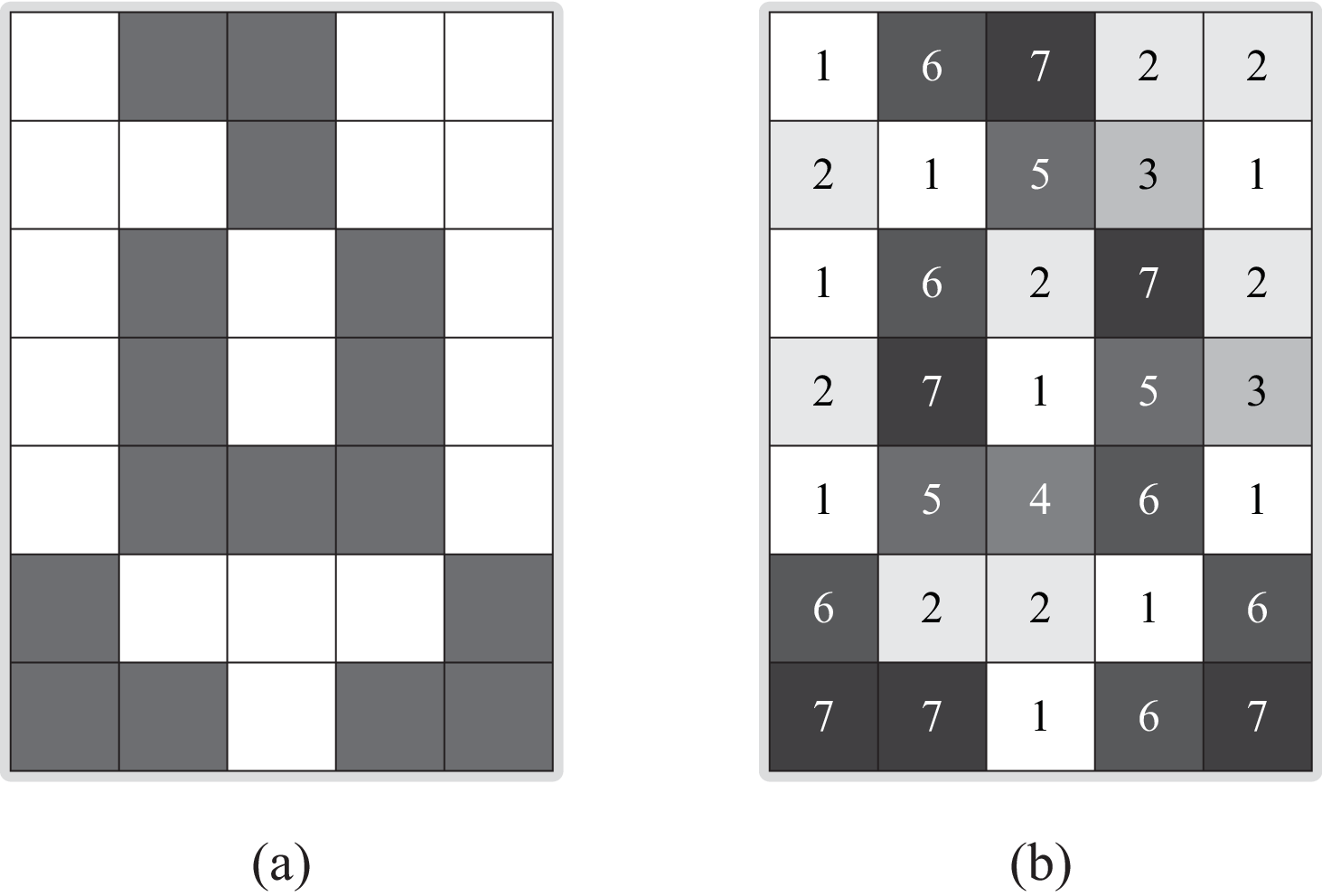
For example, the 2-coloured pattern in Figure 2a defines a 2-part partition, , say. The 7-part partition in Figure 2b is a refinement of () and in fact, is constructible (see Figure 3b) and corresponds to a minimal solution of the PATS problem defined by the pattern .
3.2 Determining constructibility
In this section we give an algorithm for deciding the constructibility of a given partition in polynomial time. To do this, we use the concept of most general (or least constraining) tile assignments. For simplicity, we assume the set of glue labels to be infinite.
Definition 2
Given a partition of the set , a most general tile assignment (MGTA) is a function such that
- A1.
When every position in is assigned a tile type according to , any two adjacent positions agree on the glue type of the side between them.
- A2.
For all assignments satisfying A1 we have11 1 To shorten the notation we write instead of .
(5) for all .
To demonstrate this concept we present a most general tile assignment for the initial partition in Figure 3a and a MGTA for the partition of Figure 2b in Figure 3b.

Given a partition and a function , we say that is obtained from by merging glues and if for all we have
| (6) |
A most general tile assignment for a partition can be found as follows. We start with a function that assigns to each tile edge a unique glue type, or in other words, a function so that the mapping is injective. Next, we go through all pairs of adjacent positions in (in some order) and require their matching sides to have the same glue type by merging the corresponding glues. This process generates a sequence of functions and terminates after steps.
Lemma 2
The above algorithm generates a most general tile assignment.
Proof
By the end, we are left with a function that satisfies property A1 by construction. To see why property A2 is satisfied, we again use the language of partitions.
Any assignment gives rise to a set of equivalence classes (or a partition) on : Elements that are assigned the same glue type reside in the same equivalence class. The initial assignment gives each part-direction pair a unique glue type, and thus, corresponds to the initial partition . In the algorithm, any glue merging operation corresponds to the combination of two equivalence classes.
The algorithm goes through a list of pairs of elements from that are required to have the same glue type. In this way, the list records necessary conditions for property A1 to hold. This is to say that every assignment satisfying A1 has to correspond to a partition that is coarser than each of the partitions in , where is the partition obtained from the initial partition by combining parts and . Since the set is a lattice, there exists a unique greatest lower bound of the partitions in . This is exactly the partition that the algorithm calculates in the form of the assignment . As a greatest lower bound, is finer than any partition corresponding to an assignment satisfying A1, but this is precisely the requirement for condition A2.∎
The above analysis also gives the following.
Corollary 1
For a given partition, MGTAs are unique up to relabeling of the glue types.
Thus, for each partition , we take the MGTA for to be some canonical representative from the class of MGTAs for .
For efficiency purposes, it is worth mentioning that MGTAs can be generated iteratively: A partition can be obtained by repeatedly combining parts starting from the initial partition :
| (7) |
As a base case, a MGTA for can be computed by the above algorithm. A MGTA for each can be computed from a MGTA for the previous partition by just a small modification: Let a MGTA be given for and suppose is obtained from by combining parts . Now, a MGTA for can be obtained from by merging tiles and , that is, merging the glue types on the four corresponding sides.
We now give the conditions for a partition to be constructible in terms of MGTAs.
Lemma 3
A partition is constructible iff the MGTA for is injective and the tile set is deterministic in the sense of Proposition 1.
Proof
“”: Let be constructible and let the MGTA for be given. Let be a deterministic TAS such that . The uniquely produced assembly of induces a tile assignment that satisfies property A1. Now using property A2 for the MGTA we see that any violation of the injectivity of or any violation of the determinism of the tile set would imply such violations for . But since corresponds to a constructible partition, no violations can occur for and thus none for .
“”: Let be an injective MGTA with deterministic tile set . Because is deterministic, we can choose glue types for a seed assembly so that the westernmost and southernmost tiles fall into place according to in the self-assembly process. The TAS , with appropriate glue strengths , then uniquely produces a terminal assembly that agrees with on . This gives , but since is injective, and so . ∎
3.3 An initial search DAG
Our algorithm performs an exhaustive search in the lattice searching for constructible partitions. In the search, we maintain and incrementally update MGTAs for every partition we visit. First, we describe simple branching rules to obtain a rooted directed acyclic graph search structure and later give rules to prune this DAG to a node-disjoint search tree.
The root of the DAG is taken to be the initial partition that is always constructible. For each partition we next define the set of children of . Our algorithm always proceeds by combining parts of the partition currently being visited, so for each we will have . Say we visit a partition . We have two possibilities:
- C1.
is constructible:
- 1.
If is not a refinement of the target pattern , that is if , we can drop this branch of the search, since no possible descendant can be a refinement of either. (i.e. )
- 2.
In case , we can use the MGTA for to give a concrete solution to the PATS problem instance defined by the colouring . To continue the search and to find more optimal solutions we consider each pair of parts in turn and recursively visit the partition where the two parts are combined. In fact, by the above analysis, it is sufficient to consider only pairs of the same colour:
(8)
- 1.
- C2.
is not constructible: In this case the MGTA for gives and for some parts . We continue the search from partition :
(9)
To guarantee that our algorithm finds the optimal solution in the case C2 above, we need the following.
Lemma 4
Let be a non-constructible partition, the MGTA for and , , parts such that and . For all constructible we have .
Proof
Let , , and be as in the statement of the lemma. Let be a constructible partition and the MGTA for . Since is coarser than we can obtain from a tile assignment such that , where is the unique part for which . The assignment has property A1 and so using A2 for the MGTA we get that
| (10) |
Now, since is constructible, the identities and can not hold for any two different parts . Looking at the definition of , we conclude that and for some . This demonstrates . ∎
3.4 Pruning the DAG to a search tree
Computational resources should be saved by not visiting any partition twice. To keep the branches in our search structure node-disjoint, we maintain a list of graphs that store restrictions on the choices the search can make.
For each partition we associate a family of undirected graphs , one for each colour region of the pattern . Every part in is represented by a vertex in the graph corresponding to the colour of the part. More formally, the vertex set is taken to be those parts for which . (So now, .) An edge indicates that the parts and are not allowed ever to be combined in the search branch in question. When we start our search with the initial partition , the edge sets are initially empty, . At each partition , the graphs have been determined inductively and the graphs for those children that we visit are defined as follows.
- D1.
If is constructible: We choose some ordering , , for similarly coloured pairs of parts. Define , to be the colour of the pair , so that . Now, we visit a partition if and only if . When we decide to visit a child partition , we define the edge sets as follows:
- 1.
We start with the graphs and add the edges for all to their corresponding graphs. Call the resulting graphs .
- 2.
Finally, as we combine the parts and to obtain the partition , we merge the vertices and in the graph (After merging, the neighbourhood of the new vertex is the union of the neighbourhoods for and in ). The graphs follow as a result.
- 1.
- D2.
If is not constructible: Here, the MGTA for suggests a single child partition for some . If , we terminate this branch of the search. Otherwise, we define the graphs to be the graphs , except that in the vertices and have to be merged.
One can see that the outcome of this pruning process is a search tree that has node-disjoint branches and one in which every possible constructible partition is still guaranteed to be found. Figure 4 presents a sketch of the search tree.
Note that we are not usually interested in finding every constructible partition , but only in finding a minimal one (in terms of ). Next, we give an efficient method to lower-bound the partition sizes of a given search branch.

3.5 The bounding function
Given a root of some subtree of the search tree, we ask: What is the smallest partition that can be found from this subtree? The nodes in the subtree rooted at consists of those partitions that can be obtained from by merging pairs of parts that are not forbidden by the graphs . This merging process halts precisely when all the graphs have beed reduced into cliques. As is well known, the size of the smallest clique that a graph can be turned into by merging non-adjacent vertices is given by the chromatic number of the graph . This immediately gives the following.
Proposition 3
For every in the subtree rooted at and constrained by , we have
| (11) |
Determining the chromatic number of an arbitrary graph is an NP-hard problem. Fortunately, we can restrict our graphs to be of a special form: graphs that consist only of a clique and some isolated vertices. For these graphs, the chromatic numbers are given by the sizes of the cliques.
To see how to maintain graphs in this form, consider as a base case the initial partition . Here, for all , so is of our special form—it has a clique of size 1. For a general partition , we go through the branching rules D1-D2.
- D1:
is constructible: Since we are allowed to choose an arbitrary ordering , , for the children , we design an ordering that preserves the special form of the graphs. For a graph of our special form, let consist of those vertices that are part of the clique in . In the algorithm, we first set for all and repeat the following process until every graph is a complete clique.
- 1.
Pick some colour and an isolated vertex .
- 2.
Process the pairs for all in some order. By the end, update to include all the edges that were just processed (the size of the clique in increases by one).
A moment’s inspection reveals that when the graphs are of our special form, so are all of the derived graphs passed on to the children of .
- 1.
- D2:
is not constructible: If the algorithm decides to continue the search from a partition , for some , we have . This means that either , in which case we are merging two isolated vertices, or one of or is part of the clique , in which case we merge an isolated vertex to the clique. In both cases, we maintain the special form in the graphs .
3.6 Traversing the search tree
When running a B&B algorithm we maintain a “current best solution” discovered so far as a global variable. This solution gives an upper bound for the minimal value of the tile set size and can be used to prune such search branches that are guaranteed (by the bounding function) to only yield solutions worse than the current best. There are two general strategies to traverse a B&B search tree: Depth-First Search and Best-First Search [2]. Our description of the search tree for the lattice is general enough to allow either of these strategies to be used in an actual implementation of the algorithm.
In the next section we give performance data on our DFS implementation of the B&B algorithm.
4 Results
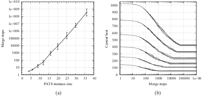

The running time of our B&B algorithm is proportional—up to a polynomial factor—to the number of partitions the algorithm visits. Hence, we measure the running time in terms of the number of merge operations performed in the search. Figure 5a presents the running time of the algorithm to find a minimal solution for random 2-coloured instances of the PATS problem. The algorithm was executed for instance sizes and ; the 20th and 80th percentiles are shown alongside the median of 21 separate runs for each instance size. For the limiting case , the algorithm spent on the order of two hours of (median) computing time on a 2,61 GHz AMD processor.
Even though B&B search is an exact method, it can be used to find approximate solutions by running it for a suitable length of time. Figure 5b illustrates how the best solution found up to a point develops as increasingly many steps of the algorithm are run. The figure provides data on random 2-coloured instances of sizes from up to . Because we begin our search from the initial partition, the best solution at the first step is precisely equal to the instance size. For each size, several different patterns were used. The algorithm was cut off after steps. By this time, an approximate reduction of 58% in the size of the tile set was achieved (cf. a reduction of 43.5% in [6]).
Next, we consider two well known examples of structured patterns: the discrete Sierpinski triangle (part of which was shown in Figure 1) and the binary counter (see Figure 1 in [12]). A tile set of size 4 is optimal for both of these patterns. First, for the Sierpinski pattern, we get a tile reduction of well over 90% (cf. 45% in [6]) in Figure 6a. We used the same cutoff threshold and instance sizes as in Figure 5b. Our description of the B&B algorithm leaves some room for randomization in deciding which search branch a DFS is to explore next. This randomization does not seem to affect the search dramatically when considering the Sierpinski pattern—the separate single runs in Figure 6a are representative of an average randomized run. By contrast, for the binary counter pattern, randomized runs for single instance size do make a difference. Figure 6b depicts several seperate runs for instance size . Here, each run brings about a reduction in solution size that oscillates between a reduction achieved on a random 2-coloured instance (5b) and a reduction achieved on the Sierpinski instance (6a). This suggests that, as is characteristic of DFS traversal, restarting the algorithm with a different random seed may help with large instances that have small optimal solutions.
5 Conclusion
We have presented an exact branch-and-bound algorithm for finding minimum-size tile sets that self-assemble a given -coloured pattern in a uniform self-assembly setting. Simulation results indicate that our algorithm is able to find provably minimal tile sets for random instances of sizes up to and can give approximate solutions for larger instances as well.
One research direction to pursue would be to study tile sets that self-assemble an infinite, but finite-period pattern. Does this generalization reduce easily to the finite case? Do there exist minimal tile sets that tile the plane aperiodically while still producing a periodic colour pattern?
References
- [1] L. Adleman, Q. Cheng, A. Goel, M.-D. Huang, D. Kempe, P. M. de Espanés, and P. W. K. Rothemund. Combinatorial optimization problems in self-assembly. In Proceedings of the 34th Annual ACM Symposium on Theory of Computing (STOC’02), pages 23–32, New York, NY, USA, 2002. ACM.
- [2] J. Clausen and M. Perregaard. On the best search strategy in parallel branch-and-bound: Best-first search versus lazy depth-first search. Annals of Operations Research, 90(0):1–17, Jan. 1999.
- [3] K. Fujibayashi, R. Hariadi, S. H. Park, E. Winfree, and S. Murata. Toward reliable algorithmic self-assembly of DNA tiles: a fixed-width cellular automaton pattern. Nano Letters, 8(7):1791–1797, July 2008.
- [4] J. I. Lathrop, J. H. Lutz, and S. M. Summers. Strict self-assembly of discrete Sierpinski triangles. Theoretical Computer Science, 410(4-5):384–405, 2009.
- [5] C. Lin, Y. Liu, S. Rinker, and H. Yan. DNA tile based self-assembly: building complex nanoarchitectures. ChemPhysChem, 7(8):1641–1647, 2006.
- [6] X. Ma and F. Lombardi. Synthesis of tile sets for DNA self-assembly. IEEE Transactions on Computer-Aided Design of Integrated Circuits and Systems, 27(5):963–967, May 2008.
- [7] X. Ma and F. Lombardi. On the computational complexity of tile set synthesis for DNA self-assembly. IEEE Transactions on Circuits and Systems II: Express Briefs, 56(1):31–35, Jan. 2009.
- [8] S. H. Park, C. Pistol, S. J. Ahn, J. H. Reif, A. R. Lebeck, C. Dwyer, and T. H. LaBean. Finite-size, fully addressable DNA tile lattices formed by hierarchical assembly procedures. Angewandte Chemie International Edition, 45(5):735–739, 2006.
- [9] S. H. Park, H. Yan, J. H. Reif, T. H. LaBean, and G. Finkelstein. Electronic nanostructures templated on self-assembled DNA scaffolds. Nanotechnology, 15:S525–S527, 2004.
- [10] P. W. K. Rothemund. Theory and Experiments in Algorithmic Self-assembly. PhD thesis, University of Southern California, 2001.
- [11] P. W. K. Rothemund. Folding DNA to create nanoscale shapes and patterns. Nature, 440(16 March 2006):297–302, 2006.
- [12] P. W. K. Rothemund and E. Winfree. The program-size complexity of self-assembled squares (extended abstract). In Proceedings of the 32nd Annual ACM Symposium on Theory of Computing (STOC’00), pages 459–468, New York, NY, USA, 2000. ACM.
- [13] E. Winfree. Algorithmic Self-Assembly of DNA. PhD thesis, California Institute of Technology, 1998.
- [14] H. Yan, S. H. Park, G. Finkelstein, J. H. Reif, and T. H. LaBean. DNA-templated self-assembly of protein arrays and highly conducive nanowires. Science, 301(26 September 2003):1882–1884, 2003.