Critical surfaces for general inhomogeneous bond percolation problems

We start with the martini lattice [32, 33] (Figure 5a), and recover the previously reported inhomogeneous bond threshold [34, 31]. To solve this problem, we could use (1) with Figure 5b, which requires a rather involved enumeration of paths on the unit cell. However, by virtue of (1), and the fact that the probabilites $P$ are all linear functions of the bond probabilities, the critical function, denoted $\mathrm{M}(p_{1},p_{2},p_{3},r_{1},r_{2},r_{3})$, is also linear in all its arguments. Furthermore, we know that setting $r_{1}=0$ results in a honeycomb lattice in which two of the bonds are doubled in series, i.e.,

$$\mathrm{M}(p_{1},p_{2},p_{3},0,r_{2},r_{3})=\mathrm{H}(p_{1},p_{2}r_{3},p_{3}r_{2}).$$

In order to satisfy this condition and linearity, the function must be of the form

$$\mathrm{M}(p_{1},p_{2},p_{3},r_{1},r_{2},r_{3})=\mathrm{H}(p_{1},p_{2}r_{3},p_{3}r_{2})+r_{1}\phi(p_{1},p_{2},p_{3},r_{2},r_{3})$$

(8)

where $\phi$ is as-yet undetermined. Setting $r_{1}=1$ gives another honeycomb lattice, this time with a more complicated vertical bond (Fig 8). The probability of crossing this bond is $p_{1}[1-(1-r_{2})(1-r_{3})]$, i.e., the $p_{1}$ bond must be open and the $r_{2}$ and $r_{3}$ bonds cannot both be closed. Thus,

$$\mathrm{M}(p_{1},p_{2},p_{3},1,r_{2},r_{3})=\mathrm{H}(p_{1}[1-(1-r_{2})(1-r_{3})],p_{2},p_{3}).$$

(9)

Using (9) in (8) allows us to determine $\phi$ uniquely. The resulting expression for $\mathrm{M}$ is

$$\mathrm{M}(p_{1},p_{2},p_{3},r_{1},r_{2},r_{3})=(1-r_{1})\mathrm{H}(p_{1},p_{2}r_{3},p_{3}r_{2})+r_{1}\mathrm{H}(p_{1}[1-(1-r_{2})(1-r_{3})],p_{2},p_{3})$$

and expanding this out leads to the final result [31, 34],

	$\displaystyle\mathrm{M}(p_{1},p_{2},p_{3},r_{1},r_{2},r_{3})$	$\displaystyle=$	$\displaystyle 1-p_{1}p_{2}r_{3}-p_{2}p_{3}r_{1}-p_{1}p_{3}r_{2}-p_{1}p_{2}r_{1}r_{2}$		(10)
		$\displaystyle-$	$\displaystyle p_{1}p_{3}r_{1}r_{3}-p_{2}p_{3}r_{2}r_{3}+p_{1}p_{2}p_{3}r_{1}r_{2}$
		$\displaystyle+$	$\displaystyle p_{1}p_{2}p_{3}r_{1}r_{3}+p_{1}p_{2}p_{3}r_{2}r_{3}+p_{1}p_{2}r_{1}r_{2}r_{3}$
		$\displaystyle+$	$\displaystyle p_{1}p_{3}r_{1}r_{2}r_{3}+p_{2}p_{3}r_{1}r_{2}r_{3}-2p_{1}p_{2}p_{3}r_{1}r_{2}r_{3}=0\ .$

Solving the polynomial $\mathrm{M}(p,p,p,p,p,p)=0$ gives the exact homogeneous bond percolation threshold, $p_{c}=1/\sqrt{2}$. Two special cases will also be useful later; the martini-A lattice (Figure 6) found by contracting the $p_{3}$ bond, $\mathrm{MA}(p_{1},p_{2},r_{1},r_{2},r_{3})\equiv\mathrm{M}(p_{1},p_{2},1,r_{1},r_{2},r_{3})$, and the martini-B lattice (Figure 7) which results from contraction of the $p_{2}$ and $p_{3}$ bonds, $\mathrm{MB}(p_{1},r_{1},r_{2},r_{3})\equiv\mathrm{M}(p_{1},1,1,r_{1},r_{2},r_{3})$.

The method we used to find this solution is somewhat less work than using (1), however its greatest virtue lies in the fact that it can be generalized to lattices that are not handled by (1). As we will show, the thresholds predicted in those cases are not exact but are always very good approximations, usually holding to $4$ or more decimal places.

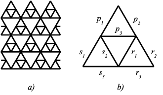
The stack of three triangles (Figure 9) will be useful in deriving the approximation for the $(3,4,6,4)$ lattice. The unit cell has $9$ probabilities, and we denote its critical function by $\mathrm{SoT}(p_{1},p_{2},p_{3},r_{1},r_{2},r_{3},s_{1},s_{2},s_{3})$ . This is a very long formula, and it is included as a text file among the source files of this submission. Here, we just report the polynomial for the homogeneous case:

$$\mathrm{SoT}(p,p,p,p,p,p,p,p,p)=1-3p^{2}-9p^{3}+3p^{4}+45p^{5}-72p^{6}+45p^{7}-12p^{8}+p^{9}=0\ .$$

The critical point of this lattice is $p_{c}=0.471629...$ [35].

This is another lattice that is helpful for the $(3,4,6,4)$ approximation. It is shown in Figure 10, which we call “rocket” from the shape of the unit cell. The critical function is denoted $\mathrm{R}(p,r,s,t,u,v,w,x)$, and once again we will forego reporting the full threshold but have included it in the supplemental material. The result for the homogeneous case is,

$$1-3p^{3}-4p^{4}+p^{5}+13p^{6}-12p^{7}+3p^{8}=0\ .$$

The critical probability is $p_{c}=0.669182...$ .

This lattice (Figure 11) will be useful when we consider the $(3^{3},4,3,4)$ lattice. It is really just a square lattice with a complicated horizontal bond. Its threshold is straightforward to find:

	$\displaystyle\mathrm{DS}(p,r,s,t,u,v)$	$\displaystyle\equiv$	$\displaystyle 1-p-st-ru-rtv-suv+rstv$		(11)
		$\displaystyle+$	$\displaystyle rstu+rsuv+rtuv+stuv-2rstuv=0.$

Bond percolation on the kagome lattice (Figure 1d) has been the subject of particular curiosity and numerous conjectures over the years [24, 36, 29]. This is the one unknown threshold for the four most basic lattices that are generally studied (the square, triangular, honeycomb, and kagome). The attraction of this problem also stems from its similarity to the double-bond honeycomb lattice, which has an exactly known bond threshold [28]. Most of the attempted solutions have been based on finding a simple connection between the two, but none have been successful (although some have been quite close).

A shortcut like the one we used for the martini lattice is possible here. We assign the probabilities as shown in Figure 12. If we set the $s_{1}$ bond probability to $0$ the result should be the martini-A lattice, so we must have

$$\mathrm{K}(r_{1},r_{2},r_{3},s_{1},s_{2},s_{3})=\mathrm{MA}(s_{3},s_{2},r_{2},r_{3},r_{1})+s_{1}\phi(r_{1},r_{2},r_{3},s_{2},s_{3}).$$

(12)

Setting this bond to $1$ gives the martini-B lattice with its $p_{1}$ bond doubled in parallel. We should therefore set $p_{1}=1-(1-s_{2})(1-s_{3})$ in the B lattice threshold:

$$\mathrm{K}(r_{1},r_{2},r_{3},1,s_{2},s_{3})=\mathrm{MB}(1-(1-s_{2})(1-s_{3}),r_{1},r_{2},r_{3}).$$

(13)

Setting $s_{1}=1$ in (12) and substituting (13) allows determination of $\phi(r_{1},r_{2},r_{3},s_{2},s_{3})$, giving

$$\mathrm{K}(r_{1},r_{2},r_{3},s_{1},s_{2},s_{3})=(1-s_{1})\mathrm{MA}(s_{3},s_{2},r_{2},r_{3},r_{1})+s_{1}\mathrm{MB}(1-(1-s_{2})(1-s_{3}),r_{1},r_{2},r_{3}).$$

(14)

After expanding, the result is:

	$\displaystyle\mathrm{K}(r_{1},r_{2},r_{3},s_{1},s_{2},s_{3})$	$\displaystyle\equiv$	$\displaystyle 1-r_{1}s_{1}-r_{2}s_{2}-r_{3}s_{3}-s_{1}r_{2}r_{3}-s_{2}r_{1}r_{3}-s_{3}r_{1}r_{2}$		(15)
		$\displaystyle-$	$\displaystyle r_{1}s_{2}s_{3}-r_{2}s_{1}s_{3}-r_{3}s_{1}s_{2}+s_{1}r_{1}r_{2}r_{3}+s_{2}r_{1}r_{2}r_{3}$
		$\displaystyle+$	$\displaystyle s_{3}r_{1}r_{2}r_{3}+r_{1}r_{2}s_{1}s_{3}+r_{1}r_{3}s_{1}s_{2}+r_{2}r_{3}s_{1}s_{2}$
		$\displaystyle+$	$\displaystyle r_{2}r_{3}s_{1}s_{3}+r_{1}r_{2}s_{2}s_{3}+r_{2}s_{1}s_{2}s_{3}+r_{3}s_{1}s_{2}s_{3}$
		$\displaystyle+$	$\displaystyle r_{1}r_{3}s_{2}s_{3}+r_{1}s_{1}s_{2}s_{3}-r_{1}r_{2}r_{3}s_{1}s_{3}-r_{1}r_{2}r_{3}s_{2}s_{3}$
		$\displaystyle-$	$\displaystyle r_{1}r_{2}r_{3}s_{1}s_{2}-r_{1}r_{2}s_{1}s_{2}s_{3}-r_{1}r_{3}s_{1}s_{2}s_{3}$
		$\displaystyle-$	$\displaystyle r_{2}r_{3}s_{1}s_{2}s_{3}+r_{1}r_{2}r_{3}s_{1}s_{2}s_{3}\ .$

This inhomogeneous threshold was reported previously in [34], but was derived by a different method. The critical probability is the solution to $\mathrm{K}(p,p,p,p,p,p)=0$, i.e.,

$$1-3p^{2}-6p^{3}+12p^{4}-6p^{5}+p^{6}=0$$

(16)

with solution in $[0,1]$, $p_{c}=0.524430...$, which is identical to the value conjectured by Wu in 1979 [24]. Two recent numerical estimates are $p_{c}=0.52440499(2)$ [5] and $p_{c}=0.52440510(5)$ [16], so we are close, but not quite right. The inhomogeneous threshold (15) is remarkable in that, absent a high-precision numerical result (which has only been available for the last twelve years [37]), it would be easy to convince oneself that it is the correct answer. It has all the necessary symmetry properties, and makes no incorrect prediction for any special case one can consider. Moreover, as is obvious from the derivation, it is the only function linear in its arguments that could possibly serve as the kagome threshold. The fact that it is incorrect means that the linearity assumption is wrong, but it is interesting that we can find such a function regardless, and that it makes a prediction so close to the correct answer. These properties are characteristic of all the criticality functions we will find here.

Equation (14) has the formal appearance of an average of two lattice thresholds. This is the general form of a linear critical surface. If we have a lattice $L_{1}$ with critical surface $f_{L_{1}}(p_{1},...,p_{n})=0$, that reduces to $L_{2}$, which is a lattice with $m<n$ bonds in its unit cell and threshold $f_{L_{2}}(r_{1},...,r_{m})$, when $p_{1}=1$ and $L_{3}$, which has $k<n$ bonds in its unit cell and threshold $f_{L_{3}}(s_{1},...,s_{k})$, when $p_{1}=0$, then we have

	$\displaystyle f_{L_{1}}(p_{1},...,p_{n})$	$\displaystyle=$	$\displaystyle p_{1}f_{L_{2}}(\rho_{1}(p_{2},...,p_{n}),...,\rho_{m}(p_{2},...,p_{n}))$		(17)
		$\displaystyle+$	$\displaystyle(1-p_{1})f_{L_{3}}(\eta_{1}(p_{2},...,p_{n}),...,\eta_{k}(p_{2},...,p_{n}))$

where $\rho_{i}$ and $\eta_{i}$ are functions that are at most first-order in their arguments. $L_{1}$ is a kind of “average” of $L_{2}$ and $L_{3}$. Equation (17) is the only way one can form a threshold that is linear in probabilities and that correctly reduces to $L_{2}$ and $L_{3}$ in the appropriate limits. This indicates that, in general, if a linear function exists that makes correct predictions in all special cases, then it is the only such function and the method of obtaining it is irrelevant.

The basic cell of the $(4,8^{2})$ (“four-eight” or “FE” lattice) lattice has six bonds and is shown in Figure 13 along with the probability assignments. Removal of the $t$ bond results in the honeycomb lattice with two doubled bonds, and setting $t=1$ gives the martini-A lattice. Equation (17) implies

$$\mathrm{FE}(p,r,s,t,u,v)=(1-t)\mathrm{H}(p,ru,sv)+t\mathrm{MA}(u,v,r,s,p).$$

Expanding gives the complete function, which will also be useful later,

	$\displaystyle\mathrm{FE}(p,r,s,t,u,v)$	$\displaystyle=$	$\displaystyle 1-(pru+stu+psv+rtv)-(rsuv+ptuv)+$
	$\displaystyle prsuv+ptruv$	$\displaystyle+$	$\displaystyle pstuv+rstuv+prstu+prstv-2prstuv=0.$

The critical polynomial $\mathrm{FE}(p,p,p,p,p,p)=0$ is then

$$1-4p^{3}-2p^{4}+6p^{5}-2p^{6}=0$$

with solution on $[0,1]$, $p_{c}=0.676835...$ . According to Parviainen [4], this lattice has $p_{c}=0.676802...$ with standard error $6.3\times 10^{-7}$. Although our answer lies outside the error bars, it does agree to four significant figures. It also lies well within the confidence interval of Riordan and Walters [20] shown in Table 1.

This threshold makes another interesting prediction. Setting $u=v=1$ gives the square lattice with four different probabilities as shown in Figure 14, and we have

$$\mathrm{CB}(p,r,s,t)\equiv 1-pr-ps-rs-pt-rt-st+prs+prt+pst+rst=0.$$

(18)

This arrangement was named the “checkerboard” by Wu [38] and he conjectured its threshold for the $q-$state Potts model based on symmetry and special cases, in much the same way as we are doing here. Our result is identical with the $q\rightarrow 1$ limit of Wu’s formula. Although his conjecture was shown to be incorrect for $q=3$ [39], our simulations suggest that it may be exact for percolation. However, proving this will require a new technique, as it is not handled by (1).

The approximation for the $(3,12^{2})$ lattice (often called the 3-12 lattice [40]) was also previously mentioned by the authors [34]. We will just repeat the result here, which we write in a factorized form to save space,

	$\displaystyle 1$	$\displaystyle-$	$\displaystyle m_{1}m_{2}(r_{3}+r_{1}r_{2}-r_{1}r_{2}r_{3})(s_{3}+s_{1}s_{2}-s_{1}s_{2}s_{3})$		(19)
		$\displaystyle-$	$\displaystyle m_{1}m_{3}(r_{2}+r_{1}r_{3}-r_{1}r_{2}r_{3})(s_{2}+s_{1}s_{3}-s_{1}s_{2}s_{3})$
		$\displaystyle-$	$\displaystyle m_{2}m_{3}(r_{1}+r_{2}r_{3}-r_{1}r_{2}r_{3})(s_{1}+s_{2}s_{3}-s_{1}s_{2}s_{3})$
		$\displaystyle+$	$\displaystyle m_{1}m_{2}m_{3}(r_{1}r_{2}+r_{1}r_{3}+r_{2}r_{3}-2r_{1}r_{2}r_{3})$
		$\displaystyle\times$	$\displaystyle(s_{1}s_{2}+s_{1}s_{3}+s_{2}s_{3}-2s_{1}s_{2}s_{3})=0\ ,$

where we have used the probability assignments from Figure 15. The polynomial for the homogeneous case factorizes to

$$(1+p-2p^{3}+p^{4})(1-p+p^{2}+p^{3}-7p^{4}+4p^{5})=0\ .$$

The part that contains the solution in $[0,1]$ is

$$1-p+p^{2}+p^{3}-7p^{4}+4p^{5}=0$$

(20)

and yields $p_{c}=0.7404233179...$ . According to Ding et al. [16], $p_{c}(3,12^{2})=0.7404207(2)$, so our approximation agrees to $5$ significant figures.

For the remaining lattices, we must employ a more brute-force method to find the critical function, requiring the use of Mathematica to perform the algebra. For the $(3^{3},4^{2})$ lattice, we consider an inhomogeneous triangular lattice, which we call the “striped” triangular lattice because the probabilities are assigned in distinct stripes (Figure 16a). The $(3^{3},4^{2})$ lattice appears when $r_{1}=0$. We start by defining the most general function that is at most first-order in its variables,

$$f(p_{1},r_{1},s_{1},p_{2},r_{2},s_{2})=\sum_{i=0}^{1}...\sum_{n=0}^{1}a_{ijklmn}p_{1}^{i}r_{1}^{j}s_{1}^{k}p_{2}^{l}r_{2}^{m}s_{2}^{n}$$

(21)

where there are $64$ $a$’s to be determined (in general, there will be $2^{n}$ coefficients, where $n$ is the number of bonds in a unit cell). However, we are free to set the constant term to $1$, because we can multiply $f=0$ by any constant and not change the threshold. Now we impose all the known symmetries and special cases onto $f$. For example, simply re-partitioning the lattice as shown in Figure 16b should not change the result, so

$$f(p_{1},r_{1},s_{1},p_{2},r_{2},s_{2})=f(p_{1},r_{1},s_{2},p_{2},r_{2},s_{1}).$$

This constraint tells us that a certain set of the $a$’s are equal to each other, reducing the number of coefficients by 16 in this case. Similarly, the threshold should be invariant under a flip about a vertical axis:

$$f(p_{1},r_{1},s_{1},p_{2},r_{2},s_{2})=f(r_{1},p_{1},s_{1},r_{2},p_{2},s_{2})$$

which eliminates another 18 coefficients. Next, there is the symmetry between the $1$ and $2$ bonds,

$$f(p_{1},r_{1},s_{1},p_{2},r_{2},s_{2})=f(p_{2},r_{2},s_{2},p_{1},r_{1},s_{1})$$

eliminating $9$ $a$’s, leaving $20$ to be determined. Setting $r_{1}=s_{1}=0$ should give the threshold for the martini-B lattice,

$$f(p_{1},0,0,p_{2},r_{2},s_{2})=\mathrm{MB}(p_{1},s_{2},p_{2},r_{2})$$

leaving $9$ undetermined coefficients. Because we are dealing with the triangular lattice $p_{1}=p_{2}=p,r_{1}=r_{2}=r,s_{1}=s_{2}=s$ should yield (6). The function $f$ will not simply reduce to the function $\mathrm{T}(p,r,s)$ because $f(p,r,s,p,r,s)$ has second-order terms. Rather, $\mathrm{T}(p,r,s)$ must factor out of the resulting expression. Because $\mathrm{T}(p,r,s)=0$ is equivalent to $p=(r+s-1)/(rs-1)$ we must have

$$f\left(\frac{r+s-1}{rs-1},r,s,\frac{r+s-1}{rs-1},r,s\right)=0.$$

This leaves only one coefficient unconstrained. We find this by observing that $r_{1}=r_{2}=0$ gives the same lattice as setting $r_{1}=p_{2}=0$, with some probabilities changed, i.e.,

$$f(p_{1},0,s_{1},p_{2},0,s_{2})=f(p_{1},0,s_{1},0,p_{2},s_{2}).$$

This finally fixes the threshold, which is given by

	$\displaystyle\mathrm{ST}(p_{1},r_{1},s_{1},p_{2},r_{2},s_{2})$	$\displaystyle\equiv$	$\displaystyle 1-s_{1}-s_{2}-p_{1}p_{2}-r_{1}r_{2}-p_{1}r_{1}-p_{2}r_{1}-p_{2}r_{2}-p_{1}r_{2}$		(22)
		$\displaystyle+$	$\displaystyle s_{1}s_{2}+p_{1}p_{2}r_{2}+p_{1}p_{2}r_{1}+p_{1}r_{1}r_{2}+p_{2}r_{1}r_{2}+p_{1}r_{1}s_{1}$
		$\displaystyle+$	$\displaystyle p_{2}r_{2}s_{1}+p_{1}r_{1}s_{2}+p_{2}r_{2}s_{2}-p_{1}r_{1}s_{1}s_{2}-p_{2}r_{2}s_{1}s_{2}$
		$\displaystyle-$	$\displaystyle p_{1}p_{2}r_{1}r_{2}s_{2}-p_{1}p_{2}r_{1}r_{2}s_{1}+p_{1}p_{2}r_{1}r_{2}s_{1}s_{2}=0$

The $(3^{3},4^{2})$ lattice is obtained by setting $r_{1}=0$:

	$\displaystyle\mathrm{TF}(p_{1},p_{2},r_{2},s_{1},s_{2})$	$\displaystyle\equiv$	$\displaystyle 1-s_{1}-s_{2}+s_{1}s_{2}-p_{1}p_{2}-p_{1}r_{2}-p_{2}r_{2}$		(23)
		$\displaystyle+$	$\displaystyle p_{2}r_{2}s_{1}+p_{2}r_{2}s_{2}+p_{1}p_{2}r_{2}-p_{2}r_{2}s_{1}s_{2}=0$

The homogeneous polynomial is

$$\mathrm{TF}(p,p,p,p,p)=1-2p-2p^{2}+3p^{3}-p^{4}=0$$

with solution on $[0,1]$ $p_{c}=0.419308...$ . Parviainen finds $p_{c}\approx 0.41964191$ with standard error $4.3\times 10^{-7}$, a difference of $0.00033$. Once again, our result is close but not in agreement with the numerical value. It may seem somewhat surprising that we could satisfy all our various criteria using only a function first-order in probabilities. What is more, we have a formula that makes predictions for cases that we did not explicitly consider in the derivation. For example, setting $s_{1}=0$ gives an inhomogeneous version of the bow-tie lattice [41], $\mathrm{BT}(p,r,s,t,u)\equiv\mathrm{ST}(t,s,0,r,p,u)$ (Figure 17), so

	$\displaystyle\mathrm{BT}(p,r,s,t,u)$	$\displaystyle=$	$\displaystyle 1-u-pr-ps-rs-pt$		(24)
		$\displaystyle-$	$\displaystyle rt-st+prs+prt+pst$
		$\displaystyle+$	$\displaystyle rst+pru+stu-prstu=0.$

Setting the probabilities equal gives

$$1-p-6p^{2}+6p^{3}-p^{5}=0$$

(25)

with $p_{c}^{\mathrm{bowtie}}=0.404518...$, which is the exact answer found by Wierman [41]. Based upon numerical studies, we believe that the more general equation (24) may also be exact [42], even though it is not obvious how to derive it using the normal duality arguments.

Another interesting prediction is found by setting $r_{1}=r_{2}=0$ (Fig 18). This again results in a square lattice, but the probabilities are assigned differently from the checkerboard. We call this the “striped” square, and the threshold is predicted by (22) to be

$$-p_{1}p_{2}+s_{1}s_{2}-s_{1}-s_{2}+1=0.$$

(26)

This formula has several interesting properties. For example, if we set $p_{1}=p_{2}=p$ and $s_{1}=s_{2}=s$ we have the standard square lattice and (26) can be factored to give

$$(1+p-s)(1-p-s)=0$$

leading to the correct threshold $1-p-s=\mathrm{S}(p,s)=0$. We can discard the first term in brackets because $s=1+p$ obviously does not give answers in $(0,1)$. Although the underlying lattice is self-dual, this assignment of probabilities is not. The dual lattice is again a square, but the inequivalent $p$ and $s$ bonds are interchanged. Our formula reflects this property too, because if we set $p_{i}\rightarrow 1-p_{i}$ and $s_{i}\rightarrow 1-s_{i}$ we indeed end up with

$$-s_{1}s_{2}+p_{1}p_{2}-p_{1}-p_{2}+1=0.$$

Finally, setting all probabilities equal leads to $p_{c}=1/2$ as required for the square lattice. Although this formula rather nicely exhibits all the required features, it does not turn out to be exact. This is easily seen by a numerical example. If we set $s_{1}=s_{2}=p_{2}=0.4$, then (26) predicts $p_{1}=0.9$. However, our numerical work [42] gives a value of $p_{1}\approx 0.9013$, which rules out this prediction.

Finally, we point out that the path we took to constrain $\mathrm{ST}(p_{1},r_{1},s_{1},p_{2},r_{2},s_{2})$ might not be the most efficient or direct; the order in which we apply the conditions is mostly just the order in which we thought of them. However, as we pointed out above, once one has found a consistent linear threshold it is the only function that has all the correct properties. The converse is not true however — two different lattices may be self-consistently represented by the same linear function. An example is equation (26), which is also the exact threshold of the square lattice with vertical bonds replaced by two in series, and horizontal bonds replaced by two in parallel (Figure (19)), i.e. $\mathrm{S}(p_{1}p_{2},1-(1-s_{1})(1-s_{2}))$.

The basic cell for the $(3,4,6,4)$ lattice of Figure 1h is shown in Figure 20. It has $12$ bonds, making it the largest cell we will consider. There are $4095$ coefficients that must be constrained (the constant is set to $1$ as usual). The constraints that fully determine the critical function are as follows:

1. 1.

   We can rotate the unit cell by $120$ degrees without changing the threshold, meaning that we have

   $$f(p_{1},p_{2},p_{3},p_{4},r_{1},r_{2},r_{3},r_{4},s_{1},s_{2},s_{3},s_{4})=f(r_{2},r_{3},r_{1},r_{4},s_{2},s_{3},s_{1},s_{4},p_{2},p_{3},p_{1},p_{4}).$$

   Rotating the opposite direction does not give any additional constraint.

2. 2.

   It is possible to re-partition the lattice, as we did in Figure 16 for the striped triangular situation, so the unit cell is still a set of three squares but the probabilities are shuffled, i.e.,

   $$f(p_{1},p_{2},p_{3},p_{4},r_{1},r_{2},r_{3},r_{4},s_{1},s_{2},s_{3},s_{4})=f(s_{1},s_{3},s_{4},s_{2},p_{4},p_{2},p_{1},p_{3},r_{2},r_{4},r_{3},r_{1}).$$

3. 3.

   We can reflect the lattice about a vertical line drawn through the middle of the unit cell, so

   $$f(p_{1},p_{2},p_{3},p_{4},r_{1},r_{2},r_{3},r_{4},s_{1},s_{2},s_{3},s_{4})=f(p_{2},p_{1},p_{3},p_{4},s_{2},s_{1},s_{3},s_{4},r_{2},r_{1},r_{3},r_{4}).$$

   Reflections about other axes do not give any further constraints.

4. 4.

   Contracting the $p_{4},r_{4},s_{4}$ bonds, i.e., setting their probabilities to $1$, results in the stack of triangles, so

   $$f(p_{1},p_{2},p_{3},1,r_{1},r_{2},r_{3},1,s_{1},s_{2},s_{3},1)=\mathrm{SoT}(p_{1},p_{2},p_{3},r_{1},r_{2},r_{3},s_{1},s_{2},s_{3}).$$

5. 5.

   Setting $s_{3},r_{3}=0$ results in the rocket lattice (Figure 10) with a complicated $v$ bond:

   $$f(p_{1},p_{2},p_{3},p_{4},r_{1},r_{2},0,r_{4},s_{1},s_{2},0,s_{4})=\mathrm{R}(r_{4},s_{4},p_{4},p_{1},p_{2},1-(1-p_{3})(1-s_{2}r_{1}),s_{1},r_{2}))$$

6. 6.

   If we set $r_{2}=r_{4}=s_{2}=s_{3}=0$, the $(4,8^{2})$ lattice with some doubled bonds results. Because we previously found the only linear function of probabilities that would qualify as that threshold, (IV.2), the current function must reduce to that one. That is,

   $$f(p_{1},p_{2},p_{3},p_{4},r_{1},0,r_{3},0,s_{1},0,0,s_{4})=\mathrm{FE}(p_{4},p_{1},p_{2},p_{3},s_{1}s_{4},r_{1}r_{3})$$

7. 7.

   A version of the kagome lattice results when we remove the $p_{3},r_{1}$, and $s_{2}$ bonds. Once again, the only consistent linear threshold is given by (15) so we expect reduction to that formula:

   $$f(p_{1},p_{2},0,p_{4},0,r_{2},r_{3},r_{4},s_{1},0,s_{3},s_{4})=\mathrm{K}(p_{4},s_{4},r_{4},s_{3}r_{3},p_{2}r_{2},s_{1}p_{1}).$$

8. 8.

   Setting $r_{2}=r_{3}=s_{1}=s_{3}=1$ gives a $(3^{3},4^{2})$ with several decorated bonds. This requires

   	$\displaystyle f(p_{1},p_{2},p_{3},p_{4},r_{1},1,1,r_{4},1,s_{2},1,s_{4})=$
   	$\displaystyle\mathrm{TF}(1-(1-p_{1})(1-p_{2}),p_{3},1-(1-r_{1})(1-r_{4}),1-(1-s_{2})(1-s_{4}),p_{4}).$

9. 9.

   Setting $p_{1}=p_{2}=r_{3}=s_{1}=1$ and $s_{4}=0$ gives a version of the dual to the $(4,8^{2})$ lattice. As such we will need

   $$\mathrm{FED}(p,r,s,t,u,v)\equiv-\mathrm{FE}(1-p,1-r,1-s,1-t,1-u,1-v).$$

   and so

   	$\displaystyle f(1,1,p_{3},p_{4},r_{1},r_{2},1,r_{4},1,s_{2},s_{3},s_{4})=$
   	$\displaystyle\mathrm{FED}(s_{4},1-(1-p_{3})(1-p_{4}),1-(1-r_{2})(1-s_{3}),r_{1},s_{2},r_{4})$

10. 10.

    We can get a version of the honeycomb lattice by assigning $p_{1}=r_{1}=r_{2}=s_{3}=s_{4}=0$:

    $$f(0,p_{2},p_{3},p_{4},0,0,r_{3},r_{4},s_{1},s_{2},0,0)=\mathrm{H}(p_{2}p_{3}p_{4},s_{1}r_{4},s_{2}r_{3})$$

11. 11.

    We now have only one coefficient left. Setting $p_{3}=p_{4}=0$ results in a 10-bond version of the dual to the bow-tie lattice, with the known threshold $p_{c}=0.595482...$ . Requiring

    $$f(p_{c},p_{c},0,0,p_{c},p_{c},p_{c},p_{c},p_{c},p_{c},p_{c},p_{c})=0$$

    (27)

    fixes the final coefficient.

All coefficients are now constrained, and the full expression, containing $879$ terms, is included in the supplemental material. The polynomial for this lattice is

$$1-6p^{3}-12p^{4}-6p^{5}+69p^{6}+60p^{7}-363p^{8}+448p^{9}-252p^{10}+66p^{11}-6p^{12}=0$$

with $p_{c}=0.524821111889...$ . Parviainen’s numerical result is $p_{c}=0.52483258$ with standard error $5.3\times 10^{-7}$. Once again we are outside the error bars but the difference is only $0.000012$ .

References

- [1] J. M. Hammersley and K. W. Morton, J. R. Stat. Soc. 16, 23 (1954).
- [2] S. R. Broadbent and J. M. Hammersley, Proc. Cambridge Phil. Soc. 53, 629 (1957).
- [3] P. N. Suding and R. M. Ziff, Phys. Rev. E 60, 275 (1999).
- [4] R. Parviainen, J. Phys. A 40, 9253 (2007).
- [5] X. Feng, Y. Deng, and H. W. J. Blöte, Phys. Rev. E 78, 031136 (2008).
- [6] R. M. Ziff and H. Gu, Phys. Rev. E 79, 020102 (2009).
- [7] A. M. Becker and R. M. Ziff, Phys. Rev. E 80, 041101 (2009).
- [8] J. A. Quintanilla and R. M. Ziff, Phys. Rev. E 76, 051115 (2007).
- [9] M. J. Lee, Phys. Rev. E 2008, 031131 (2008).
- [10] P. Grassberger, Phys. Rev. E 2003, 036101 (2003).
- [11] J.-P. Kownacki, Phys. Rev. E 77, 021121 (2008).
- [12] A. Corsi and P. D. Gujrati, Phys. Rev. E 74, 061121 (2006).
- [13] I. Kozáková, Int. J. Algebra Comput. 18, 683 (2008).
- [14] J. Li and S.-L. Zhang, Phys. Rev. E 80, 040104 (2009).
- [15] S. K. Baek, P. Minnhagen, and B. J. Kim, Phys. Rev. E 79, 011124 (2009).
- [16] C. Ding, Z. Fu, W. Guo, and F. Y. Wu, arxiv:1001.1488v1 (2010).
- [17] J. C. Wierman, Combin. Probab. Comput. 11, 629 (2002).
- [18] J. C. Wierman, Combin. Probab. Comput. 12, 95 (2003).
- [19] W. D. May and J. C. Wierman, Combin. Probab. Comput. 14, 549 (2005).
- [20] O. Riordan and M. Walters, Phys. Rev. E 76, 011110 (2007).
- [21] S. Galam and A. Mauger, Phys. Rev. E 53, 2177 (1996).
- [22] J. C. Wierman, D. P. Naor, and R. Cheng, Phys. Rev. E 72, 066116 (2005).
- [23] C. R. Scullard and R. M. Ziff, Phys. Rev. Lett. 100, 185701 (2008).
- [24] F. Y. Wu, J. Phys. C 12 (1979).
- [25] F. Y. Wu, arXiv:0911.2514 (2009).
- [26] B. Grünbaum and G. C. Shephard, Tilings and Patterns (Freeman, New York, 1987).
- [27] R. M. Ziff, Phys. Rev. E 73, 016134 (2006).
- [28] M. F. Sykes and J. W. Essam, J. Math. Phys. 5, 1117 (1964).
- [29] R. M. Ziff and C. R. Scullard, J. Phys. A 39, 15083 (2006).
- [30] L. Chayes and H. K. Lei, J. Stat. Phys. 122, 647 (2006).
- [31] F. Y. Wu, Phys. Rev. Lett. 96, 090602 (2006).
- [32] P. Fendley and K. Schoutens, Phys. Rev. Lett. 95, 046403 (2005).
- [33] C. R. Scullard, Phys. Rev. E 73, 016107 (2006).
- [34] C. R. Scullard and R. M. Ziff, Phys. Rev. E 73, 045102(R) (2006).
- [35] A. Haji-Akbari and R. M. Ziff, Phys. Rev. E 79, 021118 (2009).
- [36] C. Tsallis, J. Phys. C 15, L757 (1982).
- [37] R. M. Ziff and P. N. Suding, J. Phys. A 15, 5351 (1997).
- [38] F. Y. Wu, Rev. Mod. Phys. 54, 235 (1982).
- [39] I. G. Enting, J. Phys. A 20, L917 (1987).
- [40] J. M. Maillard, G. Rollet, and F. Y. Wu, J. Phys. A 26, L495 (1993).
- [41] J. C. Wierman, J. Phys. A 17, 1525 (1984).
- [42] R. M. Ziff, H. Gu, and C. R. Scullard, To be published (2010).