Effect of disorder and electron-phonon interaction on interlayer tunnelling current in quantum Hall bilayer.
Abstract
We study the transport properties of the quantum Hall bilayers systems looking closely at the effect that disorder and electron-phonon interaction have on the interlayer tunnelling current in the presence of an in-plane magnetic field . We find that it is important to take into account the effect of disorder and electron-phonon interactions in order to predict a finite current at a finite voltage when an in-plane magnetic field is present. We find a broadened resonant feature in the tunnelling current as a function of bias voltage, in qualitative agreement with experiments. We also find the broadening due to electron-phonon coupling has a non-monotonic dependence on , related to the geometry of the double quantum well. We also compare this with the broadening effect due to spatial fluctuations of the tunnelling amplitude. We conclude that such static disorder provides only very weak broadening of the resonant feature in the experimental range.
pacs
73.43.Jn, 73.43.Cd, 73.43.Lp, 72.10.Di,72.10.FkI Introduction
Over the last fifteen years quantum Hall bilayer systems (QHB) have been extensively studied since they are one of the few systems that show macroscopic evidence of quantum coherence. The richness of the physics of the QHB has attracted the attention of both theoretical [1, 2, 3, 4, 5, 6] and experimental studies [7, 8, 9, 10, 11]. This has led to rather rapid progress in the area. The bilayer consists of two parallel two-dimensional electron layers in a double quantum well closely separated by a distance and subjected to a magnetic field perpendicular to the plane of the layers . In this paper, we will focus on the case when each layer is a half-filled Landau level: filling factor . If the separation between layers is large they behave as two independent Fermi liquids and no quantum Hall effect is observed. When the distance between the layers becomes comparable with the magnetic length ( the system undergoes a phase transition from a compressible state at large to an incompressible state small . In the incompressible state, the system as a whole exhibits the quantum Hall effect even when interlayer tunnelling is negligible. This transition is driven by Coulomb interactions between the layers. The ground state in the quantum Hall regime is believed[3] to have a broken U(1) symmetry which leads to spontaneous interlayer phase coherence. This ground state can be described as a pseudospin ferromagnet [2] using a pseudospin picture equating electrons in the upper (lower) layer with pseudospin “up” (“down”) [2, 12], or as an excitonic superfluid[4, 13].
A series of remarkable experiments have probed the existence of this coherent phase. They show evidence for interlayer coherence with a linearly dispersing Goldstone mode [11] and counterflow superfluidity[9, 14, 15] and drag Hall voltage[16]. One piece of the experimental evidence of interlayer coherence is a sharp peak in the tunnelling current for small bias (between 10 and 100V) and low temperature. Another characteristic of the QHB that indicates the existence of phase coherence between layers is the sensitivity of the QHB to the presence of an in-plane magnetic field. The sharp peak in the tunnelling current at small bias is suppressed when a magnetic field is applied parallel to the plane of the layers. At the same time, experiments show a ’dispersive’ feature in the tunnelling current at a voltage which evolves linearly with the in-plane field . This has been interpreted as the excitation of the Goldstone mode of the excitonic superfluid at wavevector and energy given by
| (1) |
where is the velocity of the collective mode and is the flux quantum [11].
The tunnelling current can be computed using as a perturbation the interlayer hopping matrix element . For a homogeneous system in the absence of an in-plane field, Jack et al[6] found a tunnelling current proportional to at zero temperature, consistent with the observation of a region of negative differential tunnelling conductance at low temperature. However, the same calculation gives a delta function at in the tunnelling current in the presence of an in-plane field. Although the position of this feature is consistent with experiments, the experimental data does not exhibit a sharp feature even at the lowest temperatures. In this paper, we will explore sources for a finite linewidth of this feature. We find that two mechanisms should be dominant at low temperatures: tunnelling disorder and electron-phonon coupling. We will not discuss the role of vortices which could be nucleated at zero temperature by strong charge disorder or by thermal activation.
This paper is organised as follows. In the next section, we review the methodology for computing the tunnelling current as originally used by Jack et al[6]. In Section III, we discuss the effect of electron-phonon interactions on the tunnelling current. We will calculate how the magnitude and the width of the dispersive feature in the tunnelling current is affected by the electron-phonon coupling. In Section IV, we investigate the effect that an inhomogenous tunnelling amplitude over the sample has on the tunnelling current. We present the conclusions of the paper in Section V.
II Theoretical discussion
We will adopt the pseudospin picture of the quantum Hall bilayer, labelling single-particle states in the upper layer as and states in the lower layer as . We will review this framework in this section. In this picture, the system is a pseudospin ferromagnet with an easy-plane anisotropy. Furthermore, we will work with the large- generalisation of this model on a lattice which corresponds to coarse-graining the system by treating ferromagnetic patches containing electrons as lattice sites containing a large spin . The Hamiltonian can be written as:
| (2) |
where and are the pseudospin raising and lowering operators on site of a square lattice, is the exchange interaction, represents a local capacitative energy for charge imbalance. In the presence of tunnelling across the bilayer, the Hamiltonian becomes:
| (3) |
where is the interlayer tunnelling matrix element in the absence of in-plane field and is the -coordinate of the spin . We have chosen the gauge such that, in the presence of an in-plane magnetic field , the tunnelling matrix acquires a phase that varies spatially in the -direction with periodicity with as defined in (1).
The large- treatment of this model corresponds to taking to a large value while keeping and constant so that the three energy scales for exchange, interaction and tunnelling scale in the same way with . We note that in the bilayer system.
The pseudospin can be written in terms of phase and operators as
| (4) |
Semiclassically, gives the azimuthal angle of the pseudospin projected onto the -plane in spin space. They are canonical conjugate variables: . We can take the continuum limit and integrate out the (charge imbalance) fluctuations to arrive at a phase-only action[17]:
| (5) |
where , is the spin stiffness and is the Josephson length which gives the length scale over which counterflow currents decay due to tunnelling across the bilayer. If we further include a bias of across the bilayer, the only change to the action is that the cosine term in the action becomes[4, 6] . In this model, all the dynamics of the system depends on the phase . Spatial gradients in the phase correspond to counterflow in the two layers.
In the absence of tunnelling, this Lagrangian represents an easy-plane ferromagnet with spontaneously broken symmetry, i.e. a spatially uniform phase. In the presence of an in-plane magnetic field, the ground state develops spatial variations in the phase field[18, 19]. At small , the phase field increases linearly with the Aharonov-Bohm phase: . At large , the phase field cannot follow the Aharonov-Bohm phase and has only small oscillations: where is the Josephson length. The transition occurs at O(1). The Josephson length is estimated to be of the order of microns. Experimental values[11] of the in-plane field give . Therefore, the spatial fluctuations of the ground-state phase field are small. In our following calculation, we will consider quantum fluctuations as perturbations around the uniform state.
Our calculation of the quantum fluctuations in the system starts by the system in the absence of tunnelling. Then we will introduce interlayer tunnelling in perturbation theory. In the absence of tunnelling, the Hamiltonian (2) can be diagonalized
| (6) |
where the coherence factors are . This means that the elementary excitations in the pseudospin lattice system, created by the operator are long-lived pseudospin waves with energy at wavevector . At long wavelengths, the pseudospin waves have a linear dispersion, , with pseudospin wave velocity .
The operators , and all involve the creation and annihilation of pseudospin waves. Most significantly, interlayer tunnelling, , causes decay of the pseudospin waves at all wavelengths. This can be seen by examining the operator that represents electron tunnelling in the pseudospin language. From equation (4), we see that it creates perturbations in the phase and . This involves the creation and annihilation of pseudospin waves (see equation (6)). This is a consequence of the fact that tunnelling breaks the global U(1) phase invariance of the system so that Goldstone’s theorem no longer protects the long-wavelength pseudospin waves from decay.
Let us consider now the interlayer tunnelling current in the presence of an interlayer bias . The tunnelling current at site of the lattice is given by the operator . Therefore, in the continuum limit, the expectation value of the interlayer tunnelling current is[4, 6]:
| (7) |
where the expectation value is taken with respect to the full Hamiltonian as defined by (3). In a perturbative treatment of the interlayer tunnelling in the Hamiltonian , we can treat the tunnelling term in first-order perturbation theory. This gives[4, 6] a dc current proportional to :
| (8) |
where , evaluated at zero tunnelling with Hamiltonian . We can see that we are calculating the response of the system at wavevector and frequency . It can be shown that
| (9) |
where and is the propagator for the phase fluctuations at zero tunnelling.
Jack et al[6] analysed the tunnelling current at zero in-plane field. They showed that the perturbative calculation above can be understood in terms of the generation of finite-momentum pseudospin waves via the decay of the mode. Technically, this is an interpretation of (8) as a Taylor expansion of the exponential in the definition of . Each term in the Taylor expansion involving -fields represents the generation of pseudospin waves. In the absence of an in-plane field, there is no decay of the mode to a single pseudospin wave with non-zero wavevector because of momentum conservation. The most important decay channel is then the generation of a pair of pseudospin waves with equal and opposite momenta. However, in the presence of an in-plane magnetic field , the vector potential provides a momentum of , as given by equation (1), to the pseudospin system, as can be seen in the Hamiltonian (3). The generation of a single pseudospin wave at wavevector is now possible and this is the leading contribution in orders of . (In the perturbative formulation, this can be seen mathematically in (8) which tells us that we need to calculate the Fourier component of at wavevector .) For a homogeneous system, this calculation gives a current which is a delta function at :
| (10) |
In this work, we investigate possible sources of line broadening for this peak at non-zero in-plane magnetic field. We will focus on effects which do not vanish at zero temperature. In order to obtain a finite linewidth, we find that the pseudospin waves need elastic or inelastic scattering. We will discuss elastic scattering due to disorder in section IV. In section III, we will study inelastic scattering. This can arise from the generation of photons or phonons. The two mechanisms are similar. However, we will see that the energy of photons involved in this process will be much higher than the energy of the pseudospin waves. This means that the process can only be virtual. It can at most alter the dispersion relation of the pseudospin waves but cannot cause decay. Therefore, we will focus on the electron-phonon interaction in this work.
III phonon generation
In this section, we introduce interactions between phonons and pseudospin waves and study how the tunnelling current between layers is affected by the introduction of these interactions.
When electrons tunnel across the bilayer, the electron density changes, perturbing the core ions on the AlGaAs of the tunnelling barrier and thus creates phonons in the three-dimensional system in which the quantum well is embedded. For the range of values of the bias voltage used in the experiments, the most important interaction between ions in the host material and the tunnelling electrons is the deformation potential interaction [20, 21] with the acoustic phonons. We neglect optical phonons because they are at energies high compared to the electron energy at the experimental range of bias voltage.
The phonon Hamiltonian is given by:
| (11) |
where is a three-dimensional wavevector, , is the phonon frequency spectrum and and are the phonon annihilation and creation operators. We are discussing physics at wavelengths long compared to the lattice spacing of the substrate. So, we will use a simple linear dispersion for the acoustic phonon: . The electron-ion interaction takes the form:
| (12) |
where is the ion mass density, is the volume of the three-dimensional solid and is the three-dimensional electron density.
The electron density perturbation caused by tunnelling involves charge imbalance across the bilayer. It is convenient to express the density perturbation at position in terms of the -component of the pseudospin:
| (13) |
where is the three-dimensional electron density and is the one-dimensional density profile in the -direction for electrons in the upper (lower) layer, normalized to . We have scaled the density by in the spirit of the coarse-graining idea of the large- generalisation of this model, as discussed at the start of section II. It is easy to check that the above expression produce the expected three-dimensional density profile for the cases of to a balanced bilayer and completely imbalanced bilayer .
For simplicity, we approximate the electron wavefunction in the lowest subband of the single quantum well centered at by a Gaussian wavepacket:
| (14) |
where is the width of the well. (A factor of has been inserted into the exponential so that the form matches the amplitude and width of the actual wavefunction in the square well.) Using this approximation, the electron density in the Fourier representation is given by
| (15) |
where is the separation of the centres of the two quantum wells in the -direction. We have dropped terms that do not involve the pseudospin degrees of freedom, i.e. terms that do not change as a result of a tunnelling event that creates a charge imbalance across the bilayer. Note that the part proportional to vanishes as because this part represents charge imbalance and does not contribute to a uniform change in density in the -direction. In fact, the form of the -dependence in reflects the geometry of the double quantum well. There are two contributions to the geometrical form factors in this expression, analogous to the Fraunhofer diffraction pattern from a double slit in optics. The sinusoidal dependence on comes from the convolution of the two density profiles centered at and the Gaussian comes from the electron density profile in the -direction. From equations (4), (6) and (15), we see that the electron-phonon interaction in equation (12) includes the decay of one pseudospin wave with momentum into one phonon with momentum (or vice versa). This is depicted in Figure 1. There is no conservation of momentum in the -direction because translational symmetry is broken by the presence of the double quantum well. This decay of the pseudospin wave into a phonon can only occur as a real process if energy is conserved:
| (16) |
This requires the pseudospin wave velocity to be higher than the phonon velocity: . This is the case we consider here. We estimate ms-1 from the data of Spielman et al.[11] and for the sound velocity in the heterostructure[21]. On the other hand, if the phonon velocity was greater than the pseudospin wave velocity , then the process where a phonon of greater speed (or indeed a photon) can be emitted and re-absorbed is only a virtual process. This will alter the pseudospin wave spectrum but does not contribute to the tunnelling current.

We will now investigate more quantitatively how the pseudospin-phonon interaction affect the system. We proceed by integrating out the phonons to obtain an effective action. This can be performed because the electron-phonon coupling is linear in the phonon field. We obtain a retarded interaction for , the charge imbalance across the layers:
| (17) |
where
| (18) |
and ). This adds to the on-site instantaneous interaction . Integrating out , we obtain a modified phase action at zero tunnelling:
| (19) |
The decay of the pseudospin wave into a phonon is encoded in the imaginary part of . It is non-zero when :
| (20) |
For , the imaginary part of is zero. The real part of will shift the position of the peak of the tunnelling current with respect to the voltage.
The leading term on the expansion of (9) in powers of corresponds to the decay of one mode into one finite-momentum spin wave at wavevector . The contribution to the current from this term is
| (21) | |||||
with

| (22) |
The main difference between the present Green’s function and the one used by Jack et al and Balents and Radzihovsky is that this decay is affected by the phonon-electron interaction (Figure 2b) while the process considered by them is not (Figure 2a). This will give a broadened peak on the current centered at . Physically, this is a consequence of the fact that, once the spin wave is coupled to the phonons, it is no longer a sharp resonance. Mathematically, we have to inspect which includes the decay of one zero-momentum pseudospin wave with energy into a phonon with the same in-plane momentum. The poles of establish the relation between the momentum and the frequency and the integral over time in equation (21) gives the restriction for the pseudospin wave energy to . The final expression for the current is then
| (23) |
where is the pole of with a positive real part.
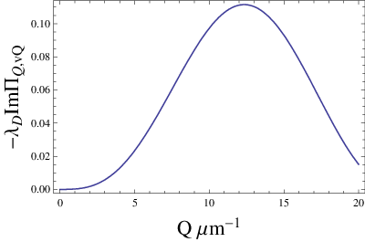
A measure of the importance of the electron-phonon coupling is the dimensionless quantity (see Fig. 3):
| (24) |
This is formally small in the large- limit. Indeed, we can check that, even if we set to unity, remains small. Neglecting the geometrical form factors, the coupling strength is given by for between 10 and 20 m-1(as probed in the experiments[11]). The geometrical form factors reduce this further. From Fig. 3, we see that the coupling is most appreciable for wavevectors in the experimental range[11] of 10 to 20m-1(with nm and nm). This corresponds to . On the other hand, the coupling can also vanish when is an integer multiple of . At these wavevectors, the electron and ion density oscillations are symmetric in the two layers and so are not excited by a tunnelling event which causes charge imbalance across the layers.
The weak electron-phonon coupling means that we can expect the pole of the Green’s function to be close to the original pseudospin wave energy: . We can approximate by and
| (25) |
This corresponds to a spin wave decay rate of . These results give us predictions for the height and width of the feature in the tunnelling current that disperses with the in-plane field as reported by Spielman et al[11]. From equation (23), the maximum value of the current occurs at . At ,
| (26) |
The width of the peak in the current as a function of the bias is similarly controlled by Im:
| (27) |
First of all, the area under the peak in the curve can be approximated by . This is proportional to so that this peak weakens as we increase the in-plane field. However, the evolution of the shape of the curve is a non-monotonic function of (see Fig. 4). The peak is sharp when electron-phonon coupling is weak, i.e. away from 10m-1. The peak is broad in the experimental regime because of the appreciable electron-phonon coupling as we noted above.


Our results are qualitatively consistent with the dispersive feature in the characteristic observed by Spielman et al[11] . This feature has been identified as due to the excitation of coherent excitations of the interlayer-coherent phase because its position moves linearly with the in-plane magnetic field. The width of the feature appears to have non-monotonic dependence on the in-plane field. It would be interesting to explore this dependence for a larger range of wavevectors in order to elucidate relaxation mechanisms in the system.
We note that our theoretical results differ in absolute magnitude from the experiments. Our current values are nearly an order of magnitude higher than the experimental values[11]. This may be due to a strongly renormalised tunnelling amplitude at low energies due to fluctuations. We also predict sharper peaks than seen in experiments. The broadest peak we obtained (which does correspond to the range of in-plane fields studied experimentally), the theory gives a width of the order of 10% of the position of the peak . See Figure 5 for a direct comparison with the differential conductance. The discrepancy may be due to other relaxation processes which contribute additively to the broadening of the peak. (We will discuss the contribution from elastic scattering in the next section.) It could also be caused by a suppression of tunnelling due to thermal[4] and quantum[6] phase fluctuations.
In summary, we have found that electron-phonon scattering may have a measurable contribution on the broadening of the coherent feature in the tunnelling characteric in the quantum Hall bilayer. In our theory, this broadening arises from the finite lifetime of the collective density excitation of the bilayer at wavevector due to the decay of electron density oscillations into lattice vibrations with the same in-plane wavevector. The effect is in fact strongest in the range of in-plane magnetic fields studied experimentally, giving a width of the order of 10% of the position of the peak .
IV Effect of disorder
We now consider the effect of disorder on the tunnelling current. Charge inhomogeneity can be present in the system in the case of strong disorder from the random distribution of dopants. This will nucleate textures in the pseudospins (merons), producing a ground state with random vorticity in the phase of counterflow superfluid. This has been investigated by Eastham, Cooper and Lee[22] who found suppressed tunnelling in the sense that the length scale for counterflow current to leak across the bilayer by tunnelling becomes enhanced by at least an order of magnitude.
In this paper, we will focus on a system of weak disorder where the ground state of the system is free of vortices. This applies to relatively clean samples which have small charge variations even on the length scale of a few magnetic lengths. We will consider in particular spatial variations in the tunnelling amplitude across the bilayer as a consequence of not having perfectly flat layers. In the pseudospin model, inhomogeneous tunnelling corresponds to inhomogeneous Zeeman coupling to the in-plane component of the pseudospin so that the Hamiltonian is:
| (28) |
where represents the fractional fluctuation around the mean tunnelling matrix element . We will model the on-site fluctuation in as Gaussian distribution with zero mean and variance . We will consider disorder which is short-ranged on the scale of the magnetic length. We can perform a perturbation theory around the zero-tunnelling ground state. After averaging over disorder, the lowest order in perturbation theory () would give a dc tunnelling current:
| (29) | |||||
This is clearly not a physical result since this expression still contains the current for the uniform system (see equation (10)) which give a delta-function response at . Therefore, we need to consider further corrections due to the disordered tunnelling strength. As we have learnt from the previous section, the scattering of the pseudospin wave at wavevector is important to consider. In the previous section, we considered scattering due to electron-phonon interactions. Here, we need to consider scattering by the disorder. This process involves terms of the form in the expansion of the Hamiltonian (28) in orders of . The matrix elements are of order and have the form:
| (30) |
The decay rate of a pseudospin wave at can be calculated from Fermi’s golden rule as . We see that we require since these collisions are elastic. We can approximate by . Averaging over disorder, we obtain a decay rate of:
| (31) |
for spatially uncorrelated disorder: .
Analogous to our previous treatment for electron-phonon coupling with a finite decay rate for the spin waves (25), this scattering rate due to disorder gives a peak for the curve of width and height:
| (32) |
This gives a field-independent peak current but a peak width that decreases with increasing .
For disorder with a correlation length of with the correlation function , we obtain:
| (33) |
As a function of the in-plane field, the peak width decreases and the peak current increases as we increase the in-plane field. This is observable if the in-plane field is large enough that becomes large compared to unity.
We can compare the width with the position of this resonant feature. For uncorrelated disorder,
| (34) |
In the experimental range, , and we expect for the validity of the perturbation theory. We see that this broadening is very weak. Consequently, the peak current is apparently very large as can be seen in our expression for the peak current (which is independent of ). Therefore, we conclude that spatial fluctuations in the tunnelling amplitude does not give rise to a strong broadening of the resonant peak. Conversely, our results indicate that, since , the broadening effect of this source of disorder is only observable at much smaller values of the in-plane field.
V Summary
We have studied in this paper extrinsic sources of scattering for the collective excitations (’spin waves’) of the counterflow superfluid, with the aim of understanding the broadened peak that disperses with in-plane field in tunnelling experiments. The peak then reflects the spectral weight of the spin waves at the wavevector .
We have concentrated on disorder and electron-phonon interaction as sources of spin wave decay and hence a broadening of the feature. Interestingly, we found that the broadening is non-monotonic and is strongest in the experimental range of in-plane fields ( 10 m-1) because the acoustic phonons emitted after the tunnelling event involve vibrations commensurate with the spacing between the two quantum wells. It will be interesting to investigate the linewidths more systematically to see if this monotonic evolution of the lineshape can be observed in experiments.
Disorder also provides broadening. We have considered fluctuations in the tunnelling amplitude across the bilayer. Our theory suggests that this provides only very weak broadening. Stronger disorder would nucleate charged quasiparticles in the system and is beyond the scope of this paper. This is discussed recently by Eastham et al[22].
However, the linewidths predicted are still nearly a factor of ten smaller than the experimental results. As mentioned above, this may be due to phase disorder due to thermal or quantum fluctuations. It will be very useful to have experimental measurements for a wider range of the magnetic fields and at lower temperatures to investigate whether electron-phonon or weak disorder are important in determining the lineshapes in this system.
Acknowledgements.
We gratefully acknowledge the financial support of EPSRC grant EPSRC-GB EP/C546814/01.References
- [1] S.M. Girvin, A.H. MacDonald and J.P. Eisenstein, in Perspectives in Quantum Hall Effects, ed. S. Das Sarma and A. Pinczuk (Wiley, New York, 1997).
- [2] K. Moon, H. Mori, K. Yang, S.M. Girvin, A.H. MacDonald, L. Zheng, D. Yoshioka, and S.C. Zhang, Phys. Rev. B 51, 5138 (1995).
- [3] X.G. Wen and A.Zee, Phys. Rev. B 47 2265 (1993).
- [4] L. Balents and L. Radzihovsky, Phys. Rev. Lett. 86, 1825 (2001).
- [5] A. Stern, S.M. Girvin, A.H. MacDonald, and N. Ma, Phys. Rev. Lett. 86, 1829(2001); M.M. Fogler and F. Wilczek, Phys. Rev. Lett. 86, 1833 (2001); Y.N. Joglekar and A.H. MacDonald,Phys. Rev. Lett. 87, 196802 (2001)
- [6] R.L. Jack, D.K.K. Lee and N.R. Cooper Phys. Rev. Lett. 93, 126803 (2004); Phys. Rev. B 71, 085310 (2005).
- [7] J.P. Eisenstein, G.S. Boebinger, L.N. Pfeiffer, K.W. West and S. He, Phys. Rev. Lett. 68,1383 (1992); J.P. Eisenstein, L.N. Pfeiffer, and K.W. West, Phys. Rev. Lett. 69, 3804 (1992).
- [8] S.Q. Murphy, J.P. Eisenstein, G.S. Boebinger,L.N. Pfeiffer, and K.W. West, Phys. Rev. Lett. 72, 728 (1994).
- [9] M. Kellogg, J.P. Eisenstein, L.N.Pfeiffer, and K.W. West, Phys. Rev. Lett. 90, 246801 (2003).
- [10] I.B. Spielman, J.P. Eisenstein, L.N. Pfeiffer, and K.W. West, Phys. Rev. Lett. 84, 5808 (2000).
- [11] I.B. Spielman, J.P. Eisenstein, L.N. Pfeiffer, and K.W. West, Phys. Rev. Lett. 87, 036803 (2001).
- [12] S.M. Girvin, in proceedings of Les Houches summer school on Topological Aspects of Low Dimensional Systems, ed. A. Comtet, T. Jolicoeur, S. Ouvry, F. David (Springer-Verlag, Berlin and Les Editions de Physique, Les Ulis, 2000).
- [13] H.A. Fertig, Phys. Rev. B. 40, 1087 (1989).
- [14] E. Tutuc, M. Shayegan and D.A. Huse, Phys. Rev. Lett. 93, 036802 (2004).
- [15] L. Tiemann, J.G.S. Lok, W. Dietsche, K. von Klitzing, K. Muraki, D. Schuh, and W. Wegscheider, Phys. Rev. B 77 033306 (2008).
- [16] L. Tiemann, W. Dietsche, M. Hauser, and K. von Klitzing, New J. Phys. 10 045018 (2008); L. Tiemann, Y. Yoon, W. Dietsche, K. von Klitzing, and W. Wegscheider, Phys. Rev. B 80, 165120 (2009).
- [17] K. Yang, K. Moon, L Zheng, A.H. MacDonald, S.M. Girvin, D. Yoshioka, and S.C. Zhang, Phys. Rev. Lett.72, 732 (1994)
- [18] P. Bak, Rep. Prog. Phys. 45 587 (1982).
- [19] C.B. Hanna, A.H. MacDonald and S.M. Girvin, Phys. Rev. B 63, 125305 (2001).
- [20] G. D. Mahan, Many-Particle Physics (Plenum, New York, 1990).
- [21] Y. Yu and M. Cardona, Fundaments of Semiconductors: Physics and Matherial Properties (Springer 2001).
- [22] P.R. Eastham, N.R. Cooper and D.K.K. Lee, Phys. Rev. B 80, 045302 (2009).