跳到论文正文
W Papers独立论文阅读器 arXiv:0911.2491 论文正文 计算阅读时间 · 0%
引用这篇论文根据当前论文元数据生成,正式投稿前建议核对。


License: arXiv.org perpetual non-exclusive license
arXiv:0911.2491v1 [astro-ph.CO] 13 Nov 2009

Cosmic String Power Spectrum, Bispectrum and Trispectrum

D.M. Regan Affiliation: Centre for Theoretical Cosmology,
Department of Applied Mathematics and Theoretical Physics,
University of Cambridge, Wilberforce Road, Cambridge CB3 0WA, United Kingdom
   E.P.S. Shellard Affiliation: Centre for Theoretical Cosmology,
Department of Applied Mathematics and Theoretical Physics,
University of Cambridge, Wilberforce Road, Cambridge CB3 0WA, United Kingdom
August 24, 2026
Abstract

We use analytic calculations of the post-recombination gravitational effects of cosmic strings to estimate the resulting CMB power spectrum, bispectrum and trispectrum. We place a particular emphasis on multipole regimes relevant for forthcoming CMB experiments, notably the Planck satellite. These calculations use a flat sky approximation, generalising previous work by integrating string contributions from last scattering to the present day, finding the dominant contributions to the correlators for multipoles l>50l>50. We find a well-behaved shape for the string bispectrum (without divergences) which is easily distinguishable from inflationary bispectra which possess significant acoustic peaks. We estimate that the nonlinearity parameter characterising the bispectrum is approximately fN​L∼−20f_{NL}\sim-20 (given present string constraints from the CMB power spectrum. We also apply these unequal time correlator methods to calculate the trispectrum for parrallelogram configurations, again valid over a large range of angular scales relevant for WMAP and Planck, as well as on very small angular scales. We find that, unlike the bispectrum which is suppressed by symmetry considerations, the trispectrum for cosmic strings is large. Our current estimate for the trispectrum parameter is τN​L∼104\tau_{NL}\sim 10^{4}, which may provide one of the strongest constraints on the string model as observational estimates for the trispectrum improve.

pacs
1

I Introduction

Cosmic strings are a common feature in fundamental cosmology scenarios, such as brane inflation [1], and they appear to be generic in realistic grand unified theories [2]. Cosmic strings leave a distinct ‘line-like’ signature in the cosmic microwave background (CMB) [3, 4] which offers one of the best prospects for their detection. Strings create this imprint after recombination by perturbing photons through relativistic gravitational effects. While inflationary fluctuations are believed to dominate the overall CMB power spectrum, current constraints suggest that up to 10% of the signal could be contributed by cosmic strings [5, 6]. A higher proportion is incompatible with WMAP because the cosmic string power spectrum around multipoles l≈200l\approx 200 is dominated by metric fluctuations with a relatively featureless spectrum, rather than the pre-recombination acoustic peaks characterising inflation. The gravitational strength of cosmic strings is determined by the parameter G​μ=(η/mP​l)2G\mu=(\eta/m_{Pl})^{2} which is the ratio of the string tension μ\mu to the square of the Planck mass mP​lm_{Pl}. The present WMAP limit on the string contribution to the CMB translates into a strong constraint on the parameter G​μ≤2.5×10⁻⁷G\mu\leq 2.5\times 10^{-7} [5].

Inflationary CMB fluctuations in the standard picture are very nearly Gaussian, so higher order correlators offer the prospect of further differentiation between these and competing signals from cosmic strings. The spherical harmonic transform of the three-point CMB correlator is the bispectrum Bl1​l2​l3B_{l_{1}l_{2}l_{3}}. Usually discussions of the bispectrum are simplified further by focusing on the nonlinearity parameter fN​Lf_{NL} which is roughly the ratio of the three point correlator to the square of the two-point correlator, that is, fN​L∼⟨ζ​ζ​ζ⟩/⟨ζ​ζ⟩2f_{NL}\sim\langle\zeta\zeta\zeta\rangle/\langle\zeta\zeta\rangle^{2} where the ζ\zeta are the primordial curvature fluctuations (dimensionless) which seed the CMB anisotropies. For a perturbative theory like inflation, we expect the second-order fluctuations ζ(2)\zeta^{(2)} to be constructed from convolutions of the linear perturbations ζ(2)∼ζ(1)∗ζ(1)\zeta^{(2)}\sim\zeta^{(1)}*\zeta^{(1)}. This implies that the leading order term in the three-point correlator can be expected to behave as ⟨ζ(1)​ζ(1)​ζ(2)⟩∼⟨ζ(1)​ζ(1)⟩2\langle\zeta^{(1)}\zeta^{(1)}\zeta^{(2)}\rangle\sim\langle\zeta^{(1)}\zeta^{(1)}\rangle^{2}, that is, fN​L∼1f_{NL}\sim 1. In fact, for standard single field inflation there is considerable further suppression from slow-roll and the primordial signal fN​L≈𝒪⁡(0.01)f_{NL}\approx{\cal O}(0.01) [7]. One can only obtain a significantly larger fN​Lf_{NL} in more exotic inflationary models with multiple scalar fields or non-canonical kinetic terms (see, for example, the reviews in [9, 8]). Similar arguments apply to the trispectrum or four-point correlator characterised by τN​L∼⟨ζ​ζ​ζ​ζ⟩/⟨ζ​ζ⟩3\tau_{NL}\sim\langle\zeta\zeta\zeta\zeta\rangle/\langle\zeta\zeta\rangle^{3} with τN​L≲1\tau_{NL}\lesssim 1 for standard single field inflation.

In contrast, the cosmic string signature has an inherently non-perturbative origin so we do not expect fN​Lf_{NL} to be small nor, more particularly, τN​L\tau_{NL}. For the higher order correlators from cosmic strings (measured relative to the string power spectrum ⟨ζ​ζ⟩c​s\langle\zeta\zeta\rangle_{cs}), the relevant scaling with the parameter G​μG\mu is fN​L∼𝒜​(G​μ)−1f_{NL}\sim{\cal A}(G\mu)^{-1} [10] and, as we shall discuss here, τN​L∼ℬ​(G​μ)2\tau_{NL}\sim{\cal B}(G\mu)^{2} with coefficients 𝒜{\cal A} and ℬ{\cal B} determined by geometric and dynamical considerations. There is a suppressed amplitude 𝒜{\cal A} for the bispectrum (due to symmetry cancellations [10]), and we contrast this here with one of the key results of this paper which is the much larger relative value of ℬ{\cal B} for the trispectrum. Here, we shall compare the higher order correlators from strings we calculate with the dominant inflationary power spectrum ⟨ζ​ζ⟩i​n​f\langle\zeta\zeta\rangle_{inf} and we will show that the trispectrum with τN​L⋙1\tau_{NL}\ggg 1 is the more likely correlator to produce the strongest constraints on cosmic strings (or with which to identify them).

In this paper, we use analytic calculations of the post-recombination string signature to estimate the power spectrum, bispectrum and trispectrum relevant for forthcoming CMB experiments, particularly the Planck satellite. We generalise previous analytic calculations of Hindmarsh and collaborators for the power spectrum [11] and bispectrum [10] based on a flat sky approximation. While this was an important first step, the summation employed was essentially confined only to strings close to the surface of last scattering and it is only relevant for very small angular scales. Here, we note that the dominant contribution on large angular scales (as well as very small angles) comes from the same gravitational GKS effects but from strings at late times well after last scattering. By integrating in time over the unequal time correlators, we obtain an approximate bispectrum valid for all l≳50l\gtrsim 50 (where the flat sky approximation breaks down), i.e. useful for both WMAP and Planck. We also apply these unequal time correlator methods to the first calculation of the trispectrum (for parralelogram configurations), which is again valid over a large range of angular scales. Our bispectrum calculation also differs from ref. [10] by eliminating the divergences they find in their Gaussian integrals for flattened triangles. We note that these are actually cut-off by the behaviour of other terms in the integrand (due to momentum constraints), yielding a finite result in this regime. The cross-sectional shape of the bispectrum we present is relatively featureless, except for a finite rise near the edges (for flattened triangles) and suppression towards the corners because of causality contraints (squeezed triangle limit). This well-behaved shape is suitable for the bispectrum estimation methods being developed for Planck and is easily distinguishable from bispectra predicted by inflation because of the absence of acoustic peaks [8]. Of course, these analytic calculations neglect important recombination effects which also provide significant contributions to the string bispectrum for 500≲l≲2000500\lesssim l\lesssim 2000. However, determining the extent to which these contributions can confuse the non-Gaussian ‘line-like’ signature of cosmic strings will be the subject of future study [12].

These results for the string bispectrum and trispectrum are important for CMB experiments and should be valid and dominant at both large and very small angular scales. While the Planck satellite does not have the resolution to see individual string signatures, it should be possible to obtain statistically significant constraints on cosmic strings that compete with limits on G​μG\mu from the power spectrum, especially for the trispectrum when these techniques are fully developed. On very small angular scales the string power spectrum begins to dominate over the inflationary signature (l>3000l>3000) because it is not influenced by exponentially decaying transfer functions. Here direct detection of ‘line-like’ signatures may prove possible provided that experiments can achieve μ​K\mu K sensitivities, as anticipated by AMI and ACT, for example. Again, searching in larger data sets for higher order correlators may provide statistically more significant results.

II Gott-Kaiser-Stebbins effect

In this section we calculate the Gott-Kaiser-Stebbins (GKS) effect which is expected to give the principle contribution to cosmic strings on subhorizon scales where we may use the flat sky approximation and can ignore the response of cosmological fluids. With these approximations the integrated Sachs Wolfe effect is equal to the temperature discontinuity in the CMB. In fact we shall show in this paper that it is the ‘late time small angular effect’ induced by the GKS effect that also dominates large angular scales for cosmic strings. The discussion here otherwise follows that of [10].

Consider a photon with 44-momentum pμ=(E,0,0,E)p_{\mu}=(E,0,0,E) and a string of coordinates Xμ​(σ,t)X^{\mu}(\sigma,t), where (σ,t)(\sigma,t) are the worldsheet coordinates of the string (with the gauge chosen such that tt corresponds to the (conformal) time coordinate). The unperturbed geodesics can be written as

Zμ=xμ+λ​pμ\displaystyle Z^{\mu}=x^{\mu}+\lambda p^{\mu}

The perturbation to the energy along the photon path (which gives the ISW effect) is

δpμ=−12∫λ1λ0hν​ρ,μ(Z(λ))pνpρdλ\displaystyle\delta p_{\mu}=-\frac{1}{2}\int_{\lambda_{1}}^{\lambda_{0}}h_{\nu\rho,\mu}(Z(\lambda))p^{\nu}p^{\rho}d\lambda (1)

where hμ​νh_{\mu\nu} is the metric perturbation which in general must be calculated. However, in refs. [13, 11] it was pointed out that we can simplify the discussion by considering

∇⟂2δ​pμ\displaystyle\mathbf{\nabla}_{\perp}^{2}\delta p_{\mu}

where ∇⟂\mathbf{\nabla}_{\perp} represents partial derivatives with respect to the transverse coordinates to the unperturbed geodesics of the photons.
Now suppose that the photon motion is in the zz-direction. This implies that (∂t−∂z)f(Z)=E−1d​fd​λ(\partial_{t}-\partial_{z})f(Z)=E^{-1}\frac{df}{d\lambda}. Also we note the following

∇2δ​pμ\displaystyle\mathbf{\nabla}^{2}\delta p_{\mu} =\displaystyle= (∂t2−∂z2−∂2)δpμ\displaystyle(\partial_{t}^{2}-\partial_{z}^{2}-\partial^{2})\delta p_{\mu}
=\displaystyle= −12∫λ0λ1dλ[(∂t+∂z)(∂t−∂z)−∂2]hν​ρ,μ(Z(λ))pνpρ\displaystyle-\frac{1}{2}\int_{\lambda_{0}}^{\lambda_{1}}d\lambda\left[(\partial_{t}+\partial_{z})(\partial_{t}-\partial_{z})-\partial^{2}\right]h_{\nu\rho,\mu}(Z(\lambda))p^{\nu}p^{\rho}

Now suppose we use the harmonic gauge for the metric perturbations. Then we have ∂2hμ​ν=16​π​G​(Tμ​ν−1/2​ημ​ν​T)\partial^{2}h_{\mu\nu}=16\pi G(T_{\mu\nu}-1/2\eta_{\mu\nu}T) which implies that we have

∇2δ​pμ\displaystyle\mathbf{\nabla}^{2}\delta p_{\mu} =\displaystyle= [12​E(∂t+∂z)hν​ρ,μpνpρ]λ1λ0+8πG∂μ∫λ0λ1dλTν​ρpνpρ.\displaystyle\left[\frac{1}{2E}(\partial_{t}+\partial_{z})h_{\nu\rho,\mu}p^{\nu}p^{\rho}\right]^{\lambda_{0}}_{\lambda_{1}}+8\pi G\partial_{\mu}\int_{\lambda_{0}}^{\lambda_{1}}d\lambda T_{\nu\rho}p^{\nu}p^{\rho}\,.

Next we define p^μ=pμ/E\hat{p}^{\mu}=p^{\mu}/E. Since we are interested in the energy we focus on the μ=0\mu=0 component. We then obtain11 1 Note that the formula (∂t−∂z)f(Z)=E−1d​fd​λ(\partial_{t}-\partial_{z})f(Z)=E^{-1}\frac{df}{d\lambda} generalises for a general photon path to (∂t+p^i∂i)=E−1dd​λ(\partial_{t}+\hat{p}^{i}\partial_{i})=E^{-1}\frac{d}{d\lambda}

Tρ​i,0​p^i\displaystyle T_{\rho i,0}\hat{p}^{i} =\displaystyle= 1E​d​Tρ​i,0​p^id​λ−Tρ​i,j​p^i​p^j\displaystyle\frac{1}{E}\frac{dT_{\rho i,0}\hat{p}^{i}}{d\lambda}-T_{\rho i,j}\hat{p}^{i}\hat{p}^{j}
⟹Tρ​ν,0​p^ν\displaystyle\implies T_{\rho\nu,0}\hat{p}^{\nu} =\displaystyle= 1E​d​Tρ​i,0​p^id​λ−Tρ​i,j​p^i​p^j+Tρ​j,j\displaystyle\frac{1}{E}\frac{dT_{\rho i,0}\hat{p}^{i}}{d\lambda}-T_{\rho i,j}\hat{p}^{i}\hat{p}^{j}+T_{\rho j,j}
=\displaystyle= ∇⟂iTρ​i+1E​d​Tρ​i,0​p^id​λ,\displaystyle\nabla_{\perp}^{i}T_{\rho i}+\frac{1}{E}\frac{dT_{\rho i,0}\hat{p}^{i}}{d\lambda}\,,

where we have used Tρ​j,j=Tρ​0,0T_{\rho j,j}=T_{\rho 0,0} in the second line and we define ∇⟂i=∂i−p^ip^j∂j\nabla_{\perp}^{i}=\partial^{i}-\hat{p}^{i}\hat{p}^{j}\partial_{j}. This leads to

∇2δ​EE=8πG∫dλE∇⟂iTi​ρp^ρ+12[(∂t+∂z)∂th^−16πGTρ​i​jp^ip^ρ]λ0λ1.\displaystyle\mathbf{\nabla}^{2}\frac{\delta E}{E}=8\pi G\int d\lambda E\nabla_{\perp}^{i}T_{i\rho}\hat{p}^{\rho}+\frac{1}{2}\left[(\partial_{t}+\partial_{z})\partial_{t}\hat{h}-16\pi GT_{\rho ij}\hat{p}^{i}\hat{p}^{\rho}\right]_{\lambda_{0}}^{\lambda_{1}}\,.

The terms in square brackets are boundary terms. These may be important at decoupling however due to the finite thickness of the last scattering surface we expect these fluctuations to be smeared out on the scales of interest and so we neglect these terms. For a string source22 2 The energy momentum tensor in the conformal gauge is Tμ​ν=∫d​t​𝑑σ​(X˙μ​X˙ν−X′μ​X′μ)​δ(4)​(x−X)T^{\mu\nu}=\int dtd\sigma(\dot{X}^{\mu}\dot{X}^{\nu}-{X^{\prime}}^{\mu}{X^{\prime}}^{\mu})\delta^{(4)}(x-X) in the light cone gauge (X0+X3=tX^{0}+X^{3}=t) this yields

∇⟂2δ=−8πGμ∫dσX˙.∇⟂δ(2)(𝐱−𝐗)\displaystyle\mathbf{\nabla}_{\perp}^{2}\delta=-8\pi G\mu\int d\sigma\dot{X}.\mathbf{\nabla}_{\perp}\delta^{(2)}(\mathbf{x-X})

where the quantities are evaluated at tr=t+z−X3​(σ,tr)t_{r}=t+z-X^{3}(\sigma,t_{r}). The wavenumber 𝐤\mathbf{k} is related to the multipole moment, ll, for l≳60l\gtrsim 60 via k2≈l⁡(l+1)/(t0−tr)2≈l⁡(l+1)/t02k^{2}\approx l(l+1)/(t_{0}-t_{r})^{2}\approx l(l+1)/t_{0}^{2}, where t0t_{0} is the conformal time today.
In Fourier space we have

−k2​δk​(tr)=i​8​π​G​μ​kA​∫d​σ​X˙A​(σ,tr)​ei​𝐤.𝐗⁡(σ,tr)\displaystyle-k^{2}\delta_{k}(t_{r})=i8\pi G\mu k^{A}\int d\sigma\dot{X}^{A}(\sigma,t_{r})e^{i\mathbf{k.X}(\sigma,t_{r})} (2)

where A=1,2A=1,2 runs over the transverse coordinates.

III Power Spectrum

III.1 Power Spectrum on small angular scales l≳500l\gtrsim 500

In order to calculate the power spectrum we find the unequal time correlator for density perturbations formed at different light cone crossing times and then we sum these up between the last scattering surface and today to get the total power spectrum P⁡(k)P(k). Defining the unequal time correlator as

P⁡(k1,t1,t2)=(2​π)2​δ(2)​(𝐤𝟏+𝐤𝟐)​⟨δ𝐤𝟏​(t1)​δ𝐤𝟐​(t2)⟩,\displaystyle P(k_{1},t_{1},t_{2})=(2\pi)^{2}\delta^{(2)}(\mathbf{k_{1}+k_{2}})\langle\delta_{\mathbf{k_{1}}}(t_{1})\delta_{\mathbf{k_{2}}}(t_{2})\rangle\,, (3)

we can find it by integrating over the string source terms (2) at the given times,

P⁡(k,t1,t2)=(8​π​G​μ)2​kA​kB𝒜​k4​∫d​σ​d​σ′​⟨X˙A​(σ,t1)​X˙B​(σ′,t2)​ei​𝐤.(𝐗⁡(σ,𝐭𝟏)−𝐗⁡(σ′,𝐭𝟐))⟩,\displaystyle P(k,t_{1},t_{2})=(8\pi G\mu)^{2}\frac{k^{A}k^{B}}{\mathcal{A}k^{4}}\int d\sigma d\sigma^{\prime}\left<\dot{X}^{A}(\sigma,t_{1})\dot{X}^{B}(\sigma^{\prime},t_{2})e^{i\mathbf{k.(X(\sigma,t_{1})-X(\sigma^{\prime},t_{2}))}}\right>\,, (4)

where 𝒜=(2​π)2​δ​(0)\mathcal{A}=(2\pi)^{2}\delta(0) is a formal area factor. We obtain the power spectrum through the sum from last scattering tl​s​st_{lss} to today t0t_{0}:

P⁡(k)=∑tl​s​st0∑tl​s​st0d​t1​d​t2​P​(k,t1,t2)\displaystyle P(k)=\sum_{t_{lss}}^{t_{0}}\sum_{t_{lss}}^{t_{0}}dt_{1}dt_{2}P(k,t_{1},t_{2})

Now we use the following three assumptions (for the network at a given time as in ref. [10]): (i) The string ensemble is a Gaussian process, i.e. we can find all the correlation functions in terms of two point correlators. (ii) We have reflection and translation invariance of the transverse coordinates. (iii) We have reflection and translation invariance of the worldsheet coordinates. This means that for equal time correlators we can write

Therefore we can write (for equal time correlators)

⟨X˙A​(σ,t)​X˙B​(σ′,t)⟩\displaystyle\left<\dot{X}^{A}(\sigma,t)\dot{X}^{B}(\sigma^{\prime},t)\right> =\displaystyle= δA​B2​V​(σ−σ′,t)\displaystyle\frac{\delta^{AB}}{2}V(\sigma-\sigma^{\prime},t)
⟨X˙A​(σ,t)​X′B​(σ′,t)⟩\displaystyle\left<\dot{X}^{A}(\sigma,t){X^{\prime}}^{B}(\sigma^{\prime},t)\right> =\displaystyle= δA​B2​M1​(σ−σ′,t)\displaystyle\frac{\delta^{AB}}{2}M_{1}(\sigma-\sigma^{\prime},t)
⟨X′A​(σ,t)​X′B​(σ′,t)⟩\displaystyle\left<{X^{\prime}}^{A}(\sigma,t){X^{\prime}}^{B}(\sigma^{\prime},t)\right> =\displaystyle= δA​B2​T​(σ−σ′,t)\displaystyle\frac{\delta^{AB}}{2}T(\sigma-\sigma^{\prime},t)

and hence we have

⟨(XA​(σ,t)−XA​(σ′,t))2⟩\displaystyle\left<(X^{A}(\sigma,t)-X^{A}(\sigma^{\prime},t))^{2}\right> =\displaystyle= ∫σ′σ∫σ′σd​σ1​d​σ2​T​(σ1−σ2,t)=:Γ⁡(σ−σ′,t)\displaystyle\int_{\sigma^{\prime}}^{\sigma}\int_{\sigma^{\prime}}^{\sigma}d\sigma_{1}d\sigma_{2}T(\sigma_{1}-\sigma_{2},t)=:\Gamma(\sigma-\sigma^{\prime},t)
⟨(XA​(σ,t)−XA​(σ′,t))​X˙A​(σ′,t)⟩\displaystyle\left<(X^{A}(\sigma,t)-X^{A}(\sigma^{\prime},t))\dot{X}^{A}(\sigma^{\prime},t)\right> =\displaystyle= ∫σ′σd​σ1​M1​(σ1−σ,t)=:Π⁡(σ−σ′,t).\displaystyle\int_{\sigma^{\prime}}^{\sigma}d\sigma_{1}M_{1}(\sigma_{1}-\sigma,t)=:\Pi(\sigma-\sigma^{\prime},t)\,.

This is an extremely powerful relation since we can use the fact that at small angles, i.e. small distances for correlators we have that Γ⁡(σ,t)∝σ2,V⁡(σ,t)∝σ0,Π⁡(σ,t)∝σ2\Gamma(\sigma,t)\propto\sigma^{2},V(\sigma,t)\propto\sigma^{0},\Pi(\sigma,t)\propto\sigma^{2}. In particular we write (for small angles)

Γ⁡(σ,t)≈t¯2​σ2,V⁡(σ,t)≈v¯2,Π⁡(σ,t)≈c02​ξ^​σ2\displaystyle\Gamma(\sigma,t)\approx\overline{t}^{2}\sigma^{2},V(\sigma,t)\approx\overline{v}^{2},\Pi(\sigma,t)\approx\frac{c_{0}}{2\hat{\xi}}\sigma^{2}

where t¯2=23−v¯2\overline{t}^{2}=\frac{2}{3}-\overline{v}^{2} and ξ^=ξ~​t\hat{\xi}=\tilde{\xi}t is the correlation length of the network which scales in (conformal) time, i.e. ξ~=constant\tilde{\xi}=\mbox{constant}. At time t≳tl​s​st\gtrsim t_{lss}, we have the following relation between the wavenumber kk and the multipole ll

k​ξ^≈l500​tl​s​st,\displaystyle k\hat{\xi}\approx\frac{l}{500}\frac{t_{lss}}{t}\,, (5)

that is, the correlation length at time t≳tl​s​st\gtrsim t_{lss} corresponds to a multipole 500​(tl​s​s/t)500(t_{lss}/t) since the correlation length at last scattering corresponds to a multipole of approximately l≈500l\approx 500. Therefore, for angular scales below 500500 we cannot integrate back to last scattering and instead to tl​s​s​(500/l)>tl​s​st_{lss}(500/l)>t_{lss}.

For unequal times, we have on small angular scales

Γ~​(σ,σ′,t1,t2)\displaystyle\tilde{\Gamma}(\sigma,\sigma^{\prime},t_{1},t_{2}) =\displaystyle= ⟨(XA​(σ,t1)−XA​(σ′,t2))2⟩≈t¯2​(σ−σ′)2+v¯2​(t1−t2)2\displaystyle\left<(X^{A}(\sigma,t_{1})-X^{A}(\sigma^{\prime},t_{2}))^{2}\right>\approx\overline{t}^{2}(\sigma-\sigma^{\prime})^{2}+\overline{v}^{2}(t_{1}-t_{2})^{2}

Hence, on small angular scales,

P(k,t1,t2)∝e−k2v¯2(t1−t2)2/4\displaystyle P(k,t_{1},t_{2})\propto e^{-k^{2}\overline{v}^{2}(t_{1}-t_{2})^{2}/4}

and so we have that P⁡(k,t1,t2)≈P⁡(k,t1,t1)P(k,t_{1},t_{2})\approx P(k,t_{1},t_{1}), such that

P⁡(k)≈∫1t0/tl​s​sd​t1​P​(k,t1,t1)\displaystyle P(k)\approx\int_{1}^{t_{0}/t_{lss}}dt_{1}P(k,t_{1},t_{1})

where we use the renormalised time t/tl​s​st/t_{lss}.

Now using

P⁡(k,t,t)=(8​π​G​μ)2​kA​kB4​𝒜​k4​∫d​σ+​∫d​σ−​⟨X˙A​(σ,t)​X˙B​(σ′,t)​ei​𝐤.(𝐗⁡(σ,𝐭)−𝐗⁡(σ′,𝐭))⟩\displaystyle P(k,t,t)=(8\pi G\mu)^{2}\frac{k^{A}k^{B}}{4\mathcal{A}k^{4}}\int d\sigma_{+}\int d\sigma_{-}\left<\dot{X}^{A}(\sigma,t)\dot{X}^{B}(\sigma^{\prime},t)e^{i\mathbf{k.(X(\sigma,t)-X(\sigma^{\prime},t))}}\right>

where σ+=σ+σ′\sigma_{+}=\sigma+\sigma^{\prime} and σ−=σ−σ′\sigma_{-}=\sigma-\sigma^{\prime}, we approximate the integral as

P⁡(k,t,t)=(8​π​G​μ)2​ℒ𝒜​12​k2​∫d​σ−​(V⁡(σ−,t)+k22​Π​(σ−,t))​exp⁡(−k24​Γ​(σ−,t))\displaystyle P(k,t,t)=(8\pi G\mu)^{2}\frac{\mathcal{L}}{\mathcal{A}}\frac{1}{2k^{2}}\int d\sigma_{-}\left(V(\sigma_{-},t)+\frac{k^{2}}{2}\Pi(\sigma_{-},t)\right)\exp\left(-\frac{k^{2}}{4}\Gamma(\sigma_{-},t)\right)

where we note that the range of integration (in σ\sigma) is limited by the length of string in the network. For large wavenumbers, k≳5000k\gtrsim 5000, we may use the small angle approximations as outlined above. However for smaller wavenumbers we can approximate this by constraining the range of σ−\sigma_{-} to (−ξ^/2,ξ^/2)(-\hat{\xi}/2,\hat{\xi}/2), since simulations show that in the range the approximations made above are reasonably accurate for k≳500k\gtrsim 500. We can make a better approximation motivated by the velocity correlator as found numerically in ref. [14]33 3 The velocity correlator here is in the light cone gauge. However the behaviour in any other temporal gauge should follow a similar behaviour.. In particular we approximate the velocity correlator (see Figure 1) to be44 4 This approximation obeys the constraint ∫d​σ​V​(σ)=0\int d\sigma V(\sigma)=0 which is a reflection of conservation of momentum in the network.

V(σ,t)≈v¯2(1−|σ|ξ^)exp(−|σ|/ξ^)\displaystyle V(\sigma,t)\approx\overline{v}^{2}\left(1-\frac{|\sigma|}{\hat{\xi}}\right)\exp\left(-|\sigma|/\hat{\xi}\right)
Refer to caption
Figure 1: Plot of the improved approximation of V⁡(σ,t)/(v¯2)V(\sigma,t)/(\overline{v}^{2}). The velocity approaches zero at the correlation length at each time tt and displays an anti-correlation which is a result of momentum conservation in the network. The plot is in units of the correlation length.

Using this approximation we may safely push the range of integration for V⁡(σ,t)V(\sigma,t) to σ∈(−∞,∞)\sigma\in(-\infty,\infty). However, using this (better) approximation here makes little difference to the total power spectrum and so we do not use it at this junction. Nevertheless, this approximation becomes very important for the bispectrum and trispectrum.

The second term in the above approximation gives a subdominant contribution to the power spectrum at all angular scales and therefore we discuss only the first term below. The power spectrum is therefore given by

k2​P​(k)≈l2​Cl≈\displaystyle k^{2}P(k)\approx l^{2}C_{l}\approx (8​π​G​μ)2​ℒ​ξ^𝒜​1ξ~​∫1t0/tl​s​sd​tt​∫0ξ~​t/2d​σ′​v¯2​π2​t¯​l​exp⁡(−t¯2​l24​σ′2)\displaystyle(8\pi G\mu)^{2}\frac{\mathcal{L}\hat{\xi}}{\mathcal{A}}\frac{1}{\tilde{\xi}}\int_{1}^{t_{0}/t_{lss}}\frac{dt}{t}\int_{0}^{\tilde{\xi}t/2}d\sigma^{\prime}\overline{v}^{2}\frac{\sqrt{\pi}}{2\overline{t}l}\exp\left(-\frac{\overline{t}^{2}l^{2}}{4}{\sigma^{\prime}}^{2}\right)
≈\displaystyle\approx (8​π​G​μ)2​ℒ​ξ^𝒜​1ξ~​π2​t¯​l​∫1t0/tl​s​sd​tt​v¯2​erf​(t¯​l​ξ~4​t)\displaystyle(8\pi G\mu)^{2}\frac{\mathcal{L}\hat{\xi}}{\mathcal{A}}\frac{1}{\tilde{\xi}}\frac{\sqrt{\pi}}{2\overline{t}l}\int_{1}^{t_{0}/t_{lss}}\frac{dt}{t}\overline{v}^{2}\mbox{erf}\left(\frac{\overline{t}l\tilde{\xi}}{4}t\right)

since the factor ℒ​ξ^/𝒜≈constant\mathcal{L}\hat{\xi}/\mathcal{A}\approx\mbox{constant} and again we use the renormalised time t/tl​s​st/t_{lss} and the renormalised worldsheet coordinate σ′=σ/t0\sigma^{\prime}=\sigma/t_{0} to simplify notation. For the purposes of finding the total power spectrum we approximate the error function by a constant - in particular, by unity since it will quickly reach this value if it is not already equal to unity at last scattering. Hence, we obtain the small angle power spectrum (l≳500l\gtrsim 500):

k2​P​(k)≈l2​Cl≈(8​π​G​μ)2​π​ℒ​ξ^2​𝒜​v¯2t¯​1l​ξ~​ln⁡(t0tl​s​s)∼l−1.\displaystyle k^{2}P(k)\approx l^{2}C_{l}\approx(8\pi G\mu)^{2}\sqrt{\pi}\frac{\mathcal{L}\hat{\xi}}{2\mathcal{A}}\frac{\overline{v}^{2}}{\overline{t}}\frac{1}{l\tilde{\xi}}\ln\left(\frac{t_{0}}{t_{lss}}\right)\sim l^{-1}\,. (6)

III.2 Power Spectrum on large angular scales, l≲500l\lesssim 500

In ref. [11], it was shown that if we compute the large angle power spectrum using the contribution of strings at the last scattering surface then k2​P​(k)∝k2k^{2}P(k)\propto k^{2} or l2​Cl∝l2l^{2}C_{l}\propto l^{2} on lengthscales above the correlation length (l≲500l\lesssim 500). However, we will show in this section that the late time small angle contribution of strings, i.e. the small angle effect of cosmic strings as the network evolves between last scattering and today, is the dominant contribution to the low ll part of the spectrum. We find this by integrating the unequal time correlator for all times between t>tl​s​st>t_{lss} and t0t_{0} and finding where the peak of the spectrum from such times is located. Such contributions are, in effect, superhorizon effects at last scattering which come inside the horizon at later times. Essentially we are tracking the evolution of the peak of the spectrum (located at l≈500l\approx 500 at last scattering) in time. Here we simply note that the contributions on superhorizon scales at a time t=tHt=t_{H} fall off sufficiently rapidly for k<a​Hk<aH that they can be neglected relative to the late time contributions t>tHt>t_{H} from subhorizon strings.

Integrating the string sources over all times since last scattering we obtain the power spectrum relevant on large angular scales (l≲500l\lesssim 500),

k2​P​(k)≈l2​Cl\displaystyle k^{2}P(k)\approx l^{2}C_{l} ≈\displaystyle\approx (8​π​G​μ)2​π​ℒ​ξ^2​𝒜​v¯2t¯​ln⁡(t0t)\displaystyle(8\pi G\mu)^{2}\sqrt{\pi}\frac{\mathcal{L}\hat{\xi}}{2\mathcal{A}}\frac{\overline{v}^{2}}{\overline{t}}\ln\left(\frac{t_{0}}{t}\right) (7)
≈\displaystyle\approx (8​π​G​μ)2​π​ℒ​ξ^2​𝒜​v¯2t¯​ln⁡(t0tl​s​s​l500)\displaystyle(8\pi G\mu)^{2}\sqrt{\pi}\frac{\mathcal{L}\hat{\xi}}{2\mathcal{A}}\frac{\overline{v}^{2}}{\overline{t}}\ln\left(\frac{t_{0}}{t_{lss}}\frac{l}{500}\right) (8)

This is only strictly valid, as mentioned above, for l≳60l\gtrsim 60 where the flat sky approximation remains good. However, it can be extrapolated to lower ll to provide useful estimates as can our subsequent results for the bispectrum and trispectrum in these regimes. From this expression and the small angle result, we see that the peak of the power spectrum lies near l≈500l\approx 500 with a logarithmic deviation from scale-invariance on large angular scales and a steeper l−1l^{-1} fall-off on smaller scales. The large angle result is qualitatively in agreement with early numerical work on this problem in ref. [15] (see, more recent results in [5]), though we note that quantitatively the rise towards a peak at l≈500l\approx 500 is much steeper for two reasons: (i) The matter-radiation transition breaks scale-invariance because the density of strings is substantially higher in the radiation era and is therefore falling through recombination and afterwards as the string slowly responds to the smooth increase in the expansion rate. (ii) We do not take into account the pre-recombination perturbations seeded in the cosmological fluid by cosmic strings which create additional intrinsic CMB anisotropies. Since the power spectrum is not our focus here in this analytic work, we leave these quantitative issues for further study elsewhere [12].

IV Bispectrum

IV.1 Bispectrum on small angular scales

The calculation above for the power spectrum (3) can be easily extended to the bispectrum by defining the analogous unequal time correlators

⟨δ𝐤1​(t1)​δ𝐤2​(t2)​δ𝐤3​(t3)⟩=(2​π)2​δ​(𝐤𝟏+𝐤𝟐+𝐤𝟑)​BT​(𝐤1,𝐤2,𝐤3,t1,t2,t3),\displaystyle\left<\delta_{\mathbf{k}_{1}}(t_{1})\delta_{\mathbf{k}_{2}}(t_{2})\delta_{\mathbf{k}_{3}}(t_{3})\right>=(2\pi)^{2}\delta(\mathbf{k_{1}+k_{2}+k_{3}})B^{T}(\mathbf{k}_{1},\mathbf{k}_{2},\mathbf{k}_{3},t_{1},t_{2},t_{3})\,,

which are again found by integrating over the string sources

BT​(𝐤1,𝐤2,𝐤3,t1,t2,t3)=\displaystyle B^{T}(\mathbf{k}_{1},\mathbf{k}_{2},\mathbf{k}_{3},t_{1},t_{2},t_{3})=
i​(8​π​G​μ)3​1𝒜​k1A​k2B​k3Ck12​k22​k32​∫d​σ1​d​σ2​d​σ3​⟨X˙A​(σ1,t1)​X˙B​(σ2,t2)​X˙C​(σ3,t3)​ei​𝐤𝐚.𝐗𝐚⟩\displaystyle i(8\pi G\mu)^{3}\frac{1}{\mathcal{A}}\frac{k_{1}^{A}k_{2}^{B}k_{3}^{C}}{k_{1}^{2}k_{2}^{2}k_{3}^{2}}\int d\sigma_{1}d\sigma_{2}d\sigma_{3}\left<\dot{X}^{A}(\sigma_{1},t_{1})\dot{X}^{B}(\sigma_{2},t_{2})\dot{X}^{C}(\sigma_{3},t_{3})e^{i\mathbf{k_{a}.X_{a}}}\right>

where a=1,2,3a=1,2,3. As for the power spectrum, the bispectrum is found by integration of the unequal time bispectrum between last scattering and today ti∈[tl​s​s,t0]t_{i}\in[t_{lss},t_{0}]. A similar calculation to this was carried out in [10], except that the contribution was considered to be dominated by the strings near the last scattering surface i.e. t≈tl​s​st\approx t_{lss}. Just for clarity at the outset we present some of our notation. We are concerned with triangles formed by the three wavevectors 𝐤1,𝐤2,𝐤3{\bf k}_{1},\,{\bf k}_{2},\,{\bf k}_{3} such that 𝐤1+𝐤2+𝐤3=0{\bf k}_{1}+{\bf k}_{2}+{\bf k}_{3}=0 so we define

k1=|𝐤1|,k2=|𝐤2|,k3=|𝐤3|,κ12=𝐤1⋅𝐤2,κ23=𝐤2⋅𝐤3,κ13=𝐤1⋅𝐤3.\displaystyle k_{1}=|{\bf k}_{1}|\,,\quad k_{2}=|{\bf k}_{2}|\,,\quad k_{3}=|{\bf k}_{3}|\,,\qquad\kappa_{12}={\bf k}_{1}\cdot{\bf k}_{2}\,,\quad\kappa_{23}={\bf k}_{2}\cdot{\bf k}_{3}\,,\quad\kappa_{13}={\bf k}_{1}\cdot{\bf k}_{3}\,.

A particular concern will be the area of the triangle (especially for flattened cases where it vanishes) with

AreaΔ=14​2​(k12​k22+k22​k32+k32​k12)−k14−k24−k34=12​k12​k22−κ12​…\displaystyle{\rm Area}_{\Delta}=\frac{1}{4}\sqrt{2(k_{1}^{2}k_{2}^{2}+k_{2}^{2}k_{3}^{2}+k_{3}^{2}k_{1}^{2})-k_{1}^{4}-k_{2}^{4}-k_{3}^{4}}=\frac{1}{2}\sqrt{k_{1}^{2}k_{2}^{2}-\kappa_{12}}...
K1=2​A​r​e​aΔ/k1,K2=2​A​r​e​aΔ/k2,K3=2​A​r​e​aΔ/k3.\displaystyle K_{1}=2{\rm Area}_{\Delta}/k_{1}\,,\quad K_{2}=2{\rm Area}_{\Delta}/k_{2}\,,\quad K_{3}=2{\rm Area}_{\Delta}/k_{3}\,.

We note also that we will temporarily drop the subscript referring to time, which we will treat as dimensionless with the range of tt in [1,t0/tl​s​s][1,t_{0}/t_{lss}]. We will continue to use kk in place of ll, but their relation is given by (5)s in the flat sky approximation.

Writing CA​B​C=X˙A​(σ1)​X˙B​(σ2)​X˙C​(σ3)C^{ABC}=\dot{X}^{A}(\sigma_{1})\dot{X}^{B}(\sigma_{2})\dot{X}^{C}(\sigma_{3}) and D=ka.XaD=k_{a}.X_{a}, and again using the assumption of a Gaussian process we find that

⟨CA​B​C​ei​D⟩=i⁡(⟨CA​B​C​D⟩−⟨X˙A​(σ1)​D⟩​⟨X˙B​(σ2)​D⟩​⟨X˙C​(σ3)​D⟩)​e−D22\displaystyle\left<C^{ABC}e^{iD}\right>=i\left(\left<C^{ABC}D\right>-\left<\dot{X}^{A}(\sigma_{1})D\right>\left<\dot{X}^{B}(\sigma_{2})D\right>\left<\dot{X}^{C}(\sigma_{3})D\right>\right)e^{-\frac{D^{2}}{2}}

Now writing X˙1=X˙​(σ1)\dot{X}_{1}=\dot{X}(\sigma_{1}), etc we have

⟨CA​B​C​D⟩\displaystyle\left<C^{ABC}D\right> =\displaystyle= ⟨X˙1AX˙2B⟩⟨X˙3C𝐤𝐚.𝐗𝐚⟩+⟨X˙1AX˙3C⟩⟨X˙2B𝐤𝐚.𝐗𝐚⟩\displaystyle\left<\dot{X}_{1}^{A}\dot{X}_{2}^{B}\right>\left<\dot{X}_{3}^{C}\mathbf{k_{a}.X_{a}}\right>+\left<\dot{X}_{1}^{A}\dot{X}_{3}^{C}\right>\left<\dot{X}_{2}^{B}\mathbf{k_{a}.X_{a}}\right>
+⟨X˙2BX˙3C⟩⟨X˙1A𝐤𝐚.𝐗𝐚⟩\displaystyle+\left<\dot{X}_{2}^{B}\dot{X}_{3}^{C}\right>\left<\dot{X}_{1}^{A}\mathbf{k_{a}.X_{a}}\right>
=\displaystyle= δA​B2​V​(σ1−σ2)​[⟨X˙3C​k1D​(X1D−X3D)+X˙3C​k2D​(X2D−X3D)⟩]+…\displaystyle\frac{\delta^{AB}}{2}V(\sigma_{1}-\sigma_{2})\left[\left<\dot{X}_{3}^{C}k_{1}^{D}(X_{1}^{D}-X_{3}^{D})+\dot{X}_{3}^{C}k_{2}^{D}(X_{2}^{D}-X_{3}^{D})\right>\right]+\dots
=\displaystyle= δA​B4​V​(σ1−σ2)​[k1C​Π​(σ1−σ3)+k2C​Π​(σ2−σ3)]\displaystyle\frac{\delta^{AB}}{4}V(\sigma_{1}-\sigma_{2})\left[k_{1}^{C}\Pi(\sigma_{1}-\sigma_{3})+k_{2}^{C}\Pi(\sigma_{2}-\sigma_{3})\right]
+δA​C4​V​(σ1−σ3)​[k1B​Π​(σ1−σ2)+k3B​Π​(σ3−σ2)]\displaystyle+\frac{\delta^{AC}}{4}V(\sigma_{1}-\sigma_{3})\left[k_{1}^{B}\Pi(\sigma_{1}-\sigma_{2})+k_{3}^{B}\Pi(\sigma_{3}-\sigma_{2})\right]
+δB​C4​V​(σ2−σ3)​[k2A​Π​(σ2−σ1)+k3A​Π​(σ3−σ1)]\displaystyle+\frac{\delta^{BC}}{4}V(\sigma_{2}-\sigma_{3})\left[k_{2}^{A}\Pi(\sigma_{2}-\sigma_{1})+k_{3}^{A}\Pi(\sigma_{3}-\sigma_{1})\right]

and

⟨D2⟩\displaystyle\left<D^{2}\right> =\displaystyle= ⟨𝐤𝐚.𝐗𝐚𝐤𝐛.𝐗𝐛⟩\displaystyle\left<\mathbf{k_{a}.X_{a}}\mathbf{k_{b}.X_{b}}\right>
=\displaystyle= ⟨(k1A​(X1A−X3A)+k2A​(X2A−X3A))​(k2B​(X2B−X1B)+k3B​(X3B−X1B))⟩\displaystyle\left<(k_{1}^{A}(X_{1}^{A}-X_{3}^{A})+k_{2}^{A}(X_{2}^{A}-X_{3}^{A}))(k_{2}^{B}(X_{2}^{B}-X_{1}^{B})+k_{3}^{B}(X_{3}^{B}-X_{1}^{B}))\right>
=\displaystyle= −12​[κ13​Γ​(σ1−σ3)+κ23​Γ​(σ2−σ3)+κ12​Γ​(σ1−σ2)]\displaystyle-\frac{1}{2}\left[\kappa_{13}\Gamma(\sigma_{1}-\sigma_{3})+\kappa_{23}\Gamma(\sigma_{2}-\sigma_{3})+\kappa_{12}\Gamma(\sigma_{1}-\sigma_{2})\right]

where κ12=𝐤𝟏.𝐤𝟐\kappa_{12}=\mathbf{k_{1}.k_{2}}, etc. We also find that

⟨X˙iA​D⟩=∑j≠ikjA2​Πj​i⟹\displaystyle\left<\dot{X}_{i}^{A}D\right>=\sum_{j\neq i}\frac{k_{j}^{A}}{2}\Pi_{ji}\quad\implies
k1A​k2B​k3C​⟨X˙1A​D⟩​⟨X˙2B​D⟩​⟨X˙3C​D⟩=\displaystyle k_{1}^{A}k_{2}^{B}k_{3}^{C}\left<\dot{X}^{A}_{1}D\right>\left<\dot{X}^{B}_{2}D\right>\left<\dot{X}^{C}_{3}D\right>=
18​(κ12​Π12+κ13​Π13)​(κ12​Π12+κ23​Π23)​(κ13​Π13+κ23​Π23)\displaystyle\qquad\qquad\qquad\frac{1}{8}(\kappa_{12}\Pi_{12}+\kappa_{13}\Pi_{13})(\kappa_{12}\Pi_{12}+\kappa_{23}\Pi_{23})(\kappa_{13}\Pi_{13}+\kappa_{23}\Pi_{23})

(where we use the notation Πi​j=Π⁡(σi−σj)\Pi_{ij}=\Pi(\sigma_{i}-\sigma_{j})). The second term is subdominant (as in the case of the power spectrum) and so we neglect it in the following.

In order to calculate this we note that only two of σ12,σ13,σ23\sigma_{12},\sigma_{13},\sigma_{23} are independent. The choice of independent variables depend on the quantities under consideration, e.g. for the term V13​Π12V_{13}\Pi_{12} we use σ12,σ13\sigma_{12},\sigma_{13} and any term involving σ23\sigma_{23} is then written in terms of these variables. Therefore the prescription is to make a transformation from σ1,σ2,σ3\sigma_{1},\sigma_{2},\sigma_{3} to these variables. Clearly one of the integrations is then independent of the two independent variables chosen and integrates to give ℒ\mathcal{L}, as in the case of the power spectrum. In the following we consider the term V13​Π12V_{13}\Pi_{12}, i.e.

∫dσ1dσ2dσ3V13Π12exp(−D2/2)=ℒ4∫dσ12dσ13V13Π12exp(−D2/2).\displaystyle\int d\sigma_{1}d\sigma_{2}d\sigma_{3}V_{13}\Pi_{12}\exp(-D^{2}/2)=\frac{\mathcal{L}}{4}\int d\sigma_{12}d\sigma_{13}V_{13}\Pi_{12}\exp(-D^{2}/2).

We can assume the small angle approximations for Γ,Π\Gamma,\Pi but as we will outline we need to use the better approximation in the case of VV, as detailed in Section 33. In order to simplify the calculation we note that

−D22\displaystyle\frac{-D^{2}}{2} ≈\displaystyle\approx t¯24​(κ12​σ122+κ13​σ132+κ23​(σ12−σ13)2)\displaystyle\frac{\overline{t}^{2}}{4}\left(\kappa_{12}\sigma_{12}^{2}+\kappa_{13}\sigma_{13}^{2}+\kappa_{23}(\sigma_{12}-\sigma_{13})^{2}\right)
≈\displaystyle\approx −t¯24​((k2​σ12−κ23k2​σ13)2+k22​k32−κ232k22​σ132).\displaystyle-\frac{\overline{t}^{2}}{4}\left((k_{2}\sigma_{12}-\frac{\kappa_{23}}{k_{2}}\sigma_{13})^{2}+\frac{k_{2}^{2}k_{3}^{2}-\kappa_{23}^{2}}{k_{2}^{2}}\sigma_{13}^{2}\right).

This indicates that we can make the integration separable using

∫dσ12dσ13V13Π12exp(−D2/2)\displaystyle\int d\sigma_{12}d\sigma_{13}V_{13}\Pi_{12}\exp(-D^{2}/2)
≈∫d​σ12​Π12​exp⁡(−t¯2​k22​σ1224)​∫d​σ13​V13​exp⁡(−t¯2​Area△2k22​σ132)\displaystyle\approx\int d\sigma_{12}\Pi_{12}\exp\left(-\frac{\overline{t}^{2}k_{2}^{2}\sigma_{12}^{2}}{4}\right)\int d\sigma_{13}V_{13}\exp\left(-\overline{t}^{2}\frac{\mbox{Area}_{\triangle}^{2}}{k_{2}^{2}}\sigma_{13}^{2}\right)
≈∫d​σ12​Π12​exp⁡(−t¯2​k22​σ1224)​∫d​σ13​V13​exp⁡(−t¯2​K22​σ1324)\displaystyle\approx\int d\sigma_{12}\Pi_{12}\exp\left(-\frac{\overline{t}^{2}k_{2}^{2}\sigma_{12}^{2}}{4}\right)\int d\sigma_{13}V_{13}\exp\left(-\frac{\overline{t}^{2}K_{2}^{2}\sigma_{13}^{2}}{4}\right)

where Area△=k22​k32−κ232/2\mbox{Area}_{\triangle}=\sqrt{k_{2}^{2}k_{3}^{2}-\kappa_{23}^{2}}/2 and (for simplicity of notation) we denote Ki=2​Area△/kiK_{i}=2\mbox{Area}_{\triangle}/k_{i}. Since KiK_{i} (divided by t0t_{0}) may be less than 500500, i.e. correspond to an angular scale below that of the correlation length then we should use a better approximation to V12V_{12}. From earlier considerations we find that

∫d​σ​Π​(σ)​exp⁡(−t¯2​k2​σ24)=c0ξ^​∫0ξ^/2d​σ​σ2​exp⁡(−t¯2​k2​σ24)\displaystyle\int d\sigma\Pi(\sigma)\exp\left(-\frac{\overline{t}^{2}k^{2}\sigma^{2}}{4}\right)=\frac{c_{0}}{\hat{\xi}}\int_{0}^{\hat{\xi}/2}d\sigma\sigma^{2}\exp\left(-\frac{\overline{t}^{2}k^{2}\sigma^{2}}{4}\right)
≈c0ξ^​2​π​erf​(k​ξ^​t¯/4)−k​ξ^​t¯​exp⁡(−(k​ξ^​t¯/4)2)k3​t¯3≡c0ξ^​1k3​t¯3​f1​(k​ξ^)\displaystyle\approx\frac{c_{0}}{\hat{\xi}}\frac{2\sqrt{\pi}\mbox{erf}(k\hat{\xi}\overline{t}/4)-k\hat{\xi}\overline{t}\exp(-(k\hat{\xi}\overline{t}/4)^{2})}{k^{3}\overline{t}^{3}}\equiv\frac{c_{0}}{\hat{\xi}}\frac{1}{k^{3}\overline{t}^{3}}f_{1}(k\hat{\xi})

and also

∫dσV(σ)exp(−t¯2​K2​σ24)≈2v¯2∫0∞dσ(1−σξ^)exp(−σ/ξ^)exp(−t¯2​K2​σ24)\displaystyle\int d\sigma V(\sigma)\exp\left(-\frac{\overline{t}^{2}K^{2}\sigma^{2}}{4}\right)\approx 2\overline{v}^{2}\int_{0}^{\infty}d\sigma\left(1-\frac{\sigma}{\hat{\xi}}\right)\exp\left(-\sigma/\hat{\xi}\right)\exp\left(-\frac{\overline{t}^{2}K^{2}\sigma^{2}}{4}\right)
≈2​v¯2​π​(2+ξ^2​K2​t¯2)​erfc​(1/(ξ^​K​t¯))​exp⁡(1/(ξ^​K​t¯))2−2​ξ^​K​t¯K3​ξ^2​t¯3≡2​v¯2K3​ξ^2​t¯3​f2​(K​ξ^)\displaystyle\approx 2\overline{v}^{2}\frac{\sqrt{\pi}(2+\hat{\xi}^{2}K^{2}\overline{t}^{2})\mbox{erfc}(1/(\hat{\xi}K\overline{t}))\exp(1/(\hat{\xi}K\overline{t}))^{2}-2\hat{\xi}K\overline{t}}{K^{3}\hat{\xi}^{2}\overline{t}^{3}}\equiv\frac{2\overline{v}^{2}}{K^{3}\hat{\xi}^{2}\overline{t}^{3}}f_{2}(K\hat{\xi})

Using this notation (i.e. the above definitions of f1f_{1} and f2f_{2}) the total bispectrum on small angular scales (for which all ki≳500k_{i}\gtrsim 500), after some algebra, reads

B⁡(k1,k2,k3)=\displaystyle B({k_{1},k_{2},k_{3}})= ∫1t0/tl​s​sdt(8πGμ)3ℒ​ξ^𝒜c0​v¯264​t¯6​ξ^41k12​k22​k32​Area△3×\displaystyle\int_{1}^{t_{0}/t_{lss}}dt(8\pi G\mu)^{3}\frac{\mathcal{L}\hat{\xi}}{\mathcal{A}}\frac{c_{0}\overline{v}^{2}}{64\overline{t}^{6}\hat{\xi}^{4}}\frac{1}{k_{1}^{2}k_{2}^{2}k_{3}^{2}\mbox{Area}_{\triangle}^{3}}\penalty\ \times (10)
(κ12​k32​f1​(k3​ξ^)​f2​(K3​ξ^)+κ13​k22​f1​(k2​ξ^)​f2​(K2​ξ^)+κ23​k12​f1​(k1​ξ^)​f2​(K1​ξ^))\displaystyle\left(\kappa_{12}k_{3}^{2}f_{1}(k_{3}\hat{\xi})f_{2}(K_{3}\hat{\xi})+\kappa_{13}k_{2}^{2}f_{1}(k_{2}\hat{\xi})f_{2}(K_{2}\hat{\xi})+\kappa_{23}k_{1}^{2}f_{1}(k_{1}\hat{\xi})f_{2}(K_{1}\hat{\xi})\right)

In order to carry out the time integration we identify ki,Kik_{i},K_{i} as angular multipoles and ξ^=ξ~​t\hat{\xi}=\tilde{\xi}t (where we use the renormalised time as usual). We have calculated the bispectrum numerically over the full range of multipoles for which the flat sky approximation is valid and the results are shown in Figures 3 and 4. The end result is a fairly featureless flat bispectrum with very localised and modest upturns for flattened triangles and suppression of squeezed triangles because of causality. This is quite unlike the inflationary bispectra found in ref. [8] and should be easily distinguishable given a sufficiently significant signal. In the analytic spirit of this paper, however, we press on to give some simple analytic approximations to the full bispectrum () in all the different regimes:

Approximation (1):

In the small angle limit at high multipoles with ki​ξ^,Ki​ξ^≳10k_{i}\hat{\xi},K_{i}\hat{\xi}\gtrsim 10 at tl​s​st_{lss} we have f1​(ki​ξ^)≈2​πf_{1}(k_{i}\hat{\xi})\approx 2\sqrt{\pi} and f2​(Ki​ξ^)≈π​ξ^2​Ki2​t¯2f_{2}(K_{i}\hat{\xi})\approx\sqrt{\pi}\hat{\xi}^{2}K_{i}^{2}\overline{t}^{2}. This then implies that

B⁡(k1,k2,k3)\displaystyle B({k_{1},k_{2},k_{3}}) ≈\displaystyle\approx −∫1t0/tl​s​sdt(8πGμ)3ℒ​ξ^𝒜c0​v¯2​π64​t¯4​ξ^2k12+k22+k32k12​k22​k32​Area△\displaystyle-\int_{1}^{t_{0}/t_{lss}}dt(8\pi G\mu)^{3}\frac{\mathcal{L}\hat{\xi}}{\mathcal{A}}\frac{c_{0}\overline{v}^{2}\pi}{64\overline{t}^{4}\hat{\xi}^{2}}\frac{k_{1}^{2}+k_{2}^{2}+k_{3}^{2}}{k_{1}^{2}k_{2}^{2}k_{3}^{2}\mbox{Area}_{\triangle}}
≈\displaystyle\approx −(8​π​G​μ)3​ℒ​ξ^𝒜​c0​v¯2​π64​t¯4​ξ~2​k12+k22+k32k12​k22​k32​Area△\displaystyle-(8\pi G\mu)^{3}\frac{\mathcal{L}\hat{\xi}}{\mathcal{A}}\frac{c_{0}\overline{v}^{2}\pi}{64\overline{t}^{4}\tilde{\xi}^{2}}\frac{k_{1}^{2}+k_{2}^{2}+k_{3}^{2}}{k_{1}^{2}k_{2}^{2}k_{3}^{2}\mbox{Area}_{\triangle}}
⟹(k12​k22​k32)2/3​B​(k1,k2,k3)\displaystyle\implies(k_{1}^{2}k_{2}^{2}k_{3}^{2})^{2/3}B(k_{1},k_{2},k_{3}) ≈\displaystyle\approx −(8​π​G​μ)3​ℒ​ξ^𝒜​c0​v¯2​π64​t¯4​ξ~2​k12+k22+k32(k12​k22​k32)1/3​Area△∝1ξ~2​l2\displaystyle-(8\pi G\mu)^{3}\frac{\mathcal{L}\hat{\xi}}{\mathcal{A}}\frac{c_{0}\overline{v}^{2}\pi}{64\overline{t}^{4}\tilde{\xi}^{2}}\frac{k_{1}^{2}+k_{2}^{2}+k_{3}^{2}}{(k_{1}^{2}k_{2}^{2}k_{3}^{2})^{1/3}\mbox{Area}_{\triangle}}\propto\frac{1}{\tilde{\xi}^{2}l^{2}}

The difference between this result and that of ref. ([10]) is due to the approximation made to make the integration over the σ\sigma coordinates separable. This has little effect on the quantitative result and we observe the same asymptotic limit.

Approximation (2):

For K​ξ^≳5K\hat{\xi}\gtrsim 5 (at the initial time ts​t​a​r​tt_{start}) and any value of kk we find that

(k12​k22​k32)2/3​B​(k1,k2,k3)≈(8​π​G​μ)3​ℒ​ξ^𝒜​c0​v¯2​π64​t¯4​ξ~2\displaystyle(k_{1}^{2}k_{2}^{2}k_{3}^{2})^{2/3}B(k_{1},k_{2},k_{3})\approx(8\pi G\mu)^{3}\frac{\mathcal{L}\hat{\xi}}{\mathcal{A}}\frac{c_{0}\overline{v}^{2}\pi}{64\overline{t}^{4}\tilde{\xi}^{2}}
5​(κ23​erf​(k1​ξ^​t¯/4)+κ13​erf​(k2​ξ^​t¯/4)+κ12​erf​(k3​ξ^​t¯/4))3​(k12​k22​k32)1/3​Area△\displaystyle\frac{5(\kappa_{23}\mbox{erf}(k_{1}\hat{\xi}\overline{t}/4)+\kappa_{13}\mbox{erf}(k_{2}\hat{\xi}\overline{t}/4)+\kappa_{12}\mbox{erf}(k_{3}\hat{\xi}\overline{t}/4))}{3(k_{1}^{2}k_{2}^{2}k_{3}^{2})^{1/3}\mbox{Area}_{\triangle}}

where km=min⁡(ki,500)k_{m}=\min(k_{i},500) tells us the earliest time, ts​t​a​r​tt_{start}, to which we can integrate back and for which km​ξ^=(km/500)​t/tl​s​s=1k_{m}\hat{\xi}=(k_{m}/500)t/t_{lss}=1 at t=ts​t​a​r​tt=t_{start}.

Approximation (3):

For the intermediate range K​ξ^∈(3,5)K\hat{\xi}\in(3,5) we find

(k12​k22​k32)2/3​B​(k1,k2,k3)≈(8​π​G​μ)3​ℒ​ξ^𝒜​c0​v¯2​π64​t¯4​ξ~2\displaystyle(k_{1}^{2}k_{2}^{2}k_{3}^{2})^{2/3}B(k_{1},k_{2},k_{3})\approx(8\pi G\mu)^{3}\frac{\mathcal{L}\hat{\xi}}{\mathcal{A}}\frac{c_{0}\overline{v}^{2}\pi}{64\overline{t}^{4}\tilde{\xi}^{2}}
5​(κ23​erf​(k1​ξ~​t¯/4)​K1​ξ^+κ13​erf​(k2​ξ^​t¯/4)​K2​ξ~+κ12​erf​(k3​ξ^​t¯/4)​K3​ξ~)3​(k12​k22​k32)1/3​Area△\displaystyle\frac{\sqrt{5}(\kappa_{23}\mbox{erf}(k_{1}\tilde{\xi}\overline{t}/4)\sqrt{K_{1}\hat{\xi}}+\kappa_{13}\mbox{erf}(k_{2}\hat{\xi}\overline{t}/4)\sqrt{K_{2}\tilde{\xi}}+\kappa_{12}\mbox{erf}(k_{3}\hat{\xi}\overline{t}/4)\sqrt{K_{3}\tilde{\xi}})}{3(k_{1}^{2}k_{2}^{2}k_{3}^{2})^{1/3}\mbox{Area}_{\triangle}}

This approximation is adjusted slightly for K​ξ^∈(1,3)K\hat{\xi}\in(1,3) where we replace erf​(k3​ξ^​t¯/4)\mbox{erf}(k_{3}\hat{\xi}\overline{t}/4) by 0.8​erf​(k3​ξ^​t¯/2.5)0.8\mbox{erf}(k_{3}\hat{\xi}\overline{t}/2.5). However since we are interested in only a quantitative approximation to the level of signal from the bispectrum we note that we can use the expression for K​ξ^∈(3,5)K\hat{\xi}\in(3,5) in the full range (1,5)(1,5).

Approximation (4):

For flattened triangles K​ξ^≲1K\hat{\xi}\lesssim 1 the behaviour of the bispectrum gives (for small angles k​ξ^≳4k\hat{\xi}\gtrsim 4) we need an improved estimate finding

(k12​k22​k32)2/3​B​(k1,k2,k3)≈(8​π​G​μ)3​ℒ​ξ^𝒜​c0​v¯2​π64​t¯4​ξ~2\displaystyle(k_{1}^{2}k_{2}^{2}k_{3}^{2})^{2/3}B(k_{1},k_{2},k_{3})\approx(8\pi G\mu)^{3}\frac{\mathcal{L}\hat{\xi}}{\mathcal{A}}\frac{c_{0}\overline{v}^{2}\pi}{64\overline{t}^{4}\tilde{\xi}^{2}}
5​(κ23​erf​(k1​ξ^​t¯/4)​K1​ξ~+κ13​erf​(k2​ξ^​t¯/4)​K2​ξ~+κ12​erf​(k3​ξ^​t¯/4)​K3​ξ~)6​(k12​k22​k32)1/3​Area△\displaystyle\frac{\sqrt{5}(\kappa_{23}\mbox{erf}(k_{1}\hat{\xi}\overline{t}/4){K_{1}\tilde{\xi}}+\kappa_{13}\mbox{erf}(k_{2}\hat{\xi}\overline{t}/4){K_{2}\tilde{\xi}}+\kappa_{12}\mbox{erf}(k_{3}\hat{\xi}\overline{t}/4){K_{3}\tilde{\xi}})}{6(k_{1}^{2}k_{2}^{2}k_{3}^{2})^{1/3}\mbox{Area}_{\triangle}}
≈(8​π​G​μ)3​ℒ​ξ^𝒜​c0​v¯2​π32​t¯4​ξ~​κ23​erf​(k1​ξ^​t¯/4)+κ13​erf​(k2​ξ^​t¯/4)+κ12​erf​(k3​ξ^​t¯/4)3​(k12​k22​k32)1/3\displaystyle\approx(8\pi G\mu)^{3}\frac{\mathcal{L}\hat{\xi}}{\mathcal{A}}\frac{c_{0}\overline{v}^{2}\pi}{32\overline{t}^{4}\tilde{\xi}}\frac{\kappa_{23}\mbox{erf}(k_{1}\hat{\xi}\overline{t}/4)+\kappa_{13}\mbox{erf}(k_{2}\hat{\xi}\overline{t}/4)+\kappa_{12}\mbox{erf}(k_{3}\hat{\xi}\overline{t}/4)}{3(k_{1}^{2}k_{2}^{2}k_{3}^{2})^{1/3}}

This approximation is further motivated by the asymptotic expansion of erfc​(x)≈exp⁡(−x2)​1π​x+…\mbox{erfc}(x)\approx\exp(-x^{2})\frac{1}{\sqrt{\pi}x}+\dots for xx large. For k​ξ^<4k\hat{\xi}<4 we note that the formula behaves more like A​p​p​r​o​x.(3)Approx.\penalty\ (3) for lower and lower values of K​ξ^K\hat{\xi} before it becomes accurate. It is important from these approximations to note that although the bispectrum grows as we approach collapsed configurations (for which Area△→0\mbox{Area}_{\triangle}\rightarrow 0) it is not divergent and attains a finite value on the boundary.

To summarise, let us provide a final simple expression which is valid over all multipoles l<2000l<2000 (e.g. relevant for both the Planck and WMAP experiments):

(k12k22k32)2/3B(k1,k2,k3)≈(8πGμ)3ℒ​ξ^𝒜c0​v¯2​π64​t¯4​ξ~2×\displaystyle(k_{1}^{2}k_{2}^{2}k_{3}^{2})^{2/3}B(k_{1},k_{2},k_{3})\approx(8\pi G\mu)^{3}\frac{\mathcal{L}\hat{\xi}}{\mathcal{A}}\frac{c_{0}\overline{v}^{2}\pi}{64\overline{t}^{4}\tilde{\xi}^{2}}\penalty\ \times (11)
5​(κ23​erf​(k1​ξ^​t¯/4)​D​(K1​ξ~)+κ13​erf​(k2​ξ^​t¯/4)​D​(K2​ξ~)+κ12​erf​(k3​ξ^​t¯/4)​D​(K3​ξ~))3​(k12​k22​k32)1/3​Area△\displaystyle\frac{5(\kappa_{23}\mbox{erf}(k_{1}\hat{\xi}\overline{t}/4)D(K_{1}\tilde{\xi})+\kappa_{13}\mbox{erf}(k_{2}\hat{\xi}\overline{t}/4)D(K_{2}\tilde{\xi})+\kappa_{12}\mbox{erf}(k_{3}\hat{\xi}\overline{t}/4)D(K_{3}\tilde{\xi}))}{3(k_{1}^{2}k_{2}^{2}k_{3}^{2})^{1/3}\mbox{Area}_{\triangle}} (12)

where the function DD is defined by

D⁡(K​ξ~)\displaystyle D(K\tilde{\xi}) =\displaystyle= 1if​K​ξ~>5\displaystyle 1\qquad\qquad\quad\mbox{if}\,\,K\tilde{\xi}>5 (13)
=\displaystyle= K​ξ~/5if​K​ξ~∈(0,5)..\displaystyle\sqrt{K\tilde{\xi}/5}\qquad\mbox{if}\,\,K\tilde{\xi}\in(0,5)\,.. (14)

Although this expression will not accurately describe the very localised upturn near the edges of tetrahedron, this region makes a negligible integrated contribution to fN​Lf_{NL}. Going further out beyond l>2000l>2000, these upturned edge regions become more significant, so we must replace the second line above (14) by the following

D⁡(K​ξ~)\displaystyle D(K\tilde{\xi}) =\displaystyle= K​ξ~/5if​K​ξ~∈(1,5),\displaystyle\sqrt{K\tilde{\xi}/5}\qquad\mbox{if}\,\,K\tilde{\xi}\in(1,5)\,,
=\displaystyle= K​ξ~/5if​K​ξ~<1..\displaystyle K\tilde{\xi}/\sqrt{5}\qquad\mbox{if}\,\,K\tilde{\xi}<1\,..

IV.2 Bispectrum on large angular scales

If min⁡ki=km≲500\min k_{i}=k_{m}\lesssim 500, then we must restrict the range of times over which we sum to (ts​t​a​r​t,t0)(t_{start},t_{0}). We find that, as in the case for the power spectrum, the bispectrum decreases as a logarithm as we restrict the range, i.e. the bispectrum ∝ln⁡((km/500)​t0/tl​s​s)≈ln⁡(km/10)\propto\ln((k_{m}/500)t_{0}/t_{lss})\approx\ln(k_{m}/10). Therefore, we can include this effect by multiplying the formulae in the previous section by ln⁡(km/10)/ln⁡(50)\ln(k_{m}/10)/\ln(50) for km≲500k_{m}\lesssim 500. The extension to large angular scales allows us to make approximations to the level of non-Gaussianity in the parameter range of Planck. In Figures 5 and 6 we illustrate k~=k1+k2+k3=c​o​n​s​t.\tilde{k}=k_{1}+k_{2}+k_{3}=const. slices through the bispectrum to reveal the cross-sectional shape using the approximations above.

IV.3 Estimator of fN​Lf_{NL}

As detailed in [16] the signal to noise ratio of the bispectrum is given by

(S/N)2=14​π​∑l1,l2,l3(2​l1+1)​(2​l2+1)​(2​l3+1)​(l1l2l3000)2​bl1,l2,l32Cl1​Cl2​Cl3\displaystyle(S/N)^{2}=\frac{1}{4\pi}\sum_{l_{1},l_{2},l_{3}}(2l_{1}+1)(2l_{2}+1)(2l_{3}+1)\left(\begin{array}[]{ccc}l_{1}&l_{2}&l_{3}\\ 0&0&0\end{array}\right)^{2}\frac{b_{l_{1},l_{2},l_{3}}^{2}}{C_{l_{1}}C_{l_{2}}C_{l_{3}}}

where bl1​l2​l3b_{l_{1}l_{2}l_{3}} corresponds to the reduced bispectrum, which is precisely the bispectrum as calculated in the flat sky limit and where we assume that the noise is cosmic variance dominated. From the images shown in the last section we see that in the range of interest for Planck we can find a reasonably accurate estimate for fN​Lf_{NL} by summing over the equal ll values. This gives

(S/N)2\displaystyle(S/N)^{2} ≈\displaystyle\approx 2π​∑ll4​(lll000)2​bl1,l2,l32Cl1​Cl2​Cl3\displaystyle\frac{2}{\pi}\sum_{l}l^{4}\left(\begin{array}[]{ccc}l&l&l\\ 0&0&0\end{array}\right)^{2}\frac{b_{l_{1},l_{2},l_{3}}^{2}}{C_{l_{1}}C_{l_{2}}C_{l_{3}}}
≈\displaystyle\approx 12​3​π5​∑l∈2​𝒵l​(l4​bl​l​l)2(l2​Cl/(2​π))3\displaystyle\frac{1}{2\sqrt{3}\pi^{5}}\sum_{l\in 2\mathcal{Z}}\frac{l(l^{4}b_{lll})^{2}}{(l^{2}C_{l}/(2\pi))^{3}}

For the local model of inflation the signal to noise ratio is proportional to fN​Lf_{NL}. Since [8] the local bispectrum is proportional to l−4l^{-4} for l≲1000l\lesssim 1000 we normalise the signal to noise ratio of cosmic strings to that of local models of inflation, for which l4​bl​l​l≈2×10⁻¹⁷​fN​Ll^{4}b_{lll}\approx 2\times 10^{-17}f_{NL}. We have computed l2​Cl/(2​π)l^{2}C_{l}/(2\pi) using CMBFAST with WMAP5 values for the parameters. Therefore, defining,

fN​L2=(S/N)2​(cosmic strings)/(S/N)2​(inflation),\displaystyle f_{NL}^{2}=(S/N)^{2(\mbox{cosmic strings})}/(S/N)^{2(\mbox{inflation})},

we plot fN​Lf_{NL} against ll for multipoles summed between 60 and ll. The fluctuations in the plot arise since cosmic strings do not strictly follow a local model and because of the transfer functions appearing in the ClC_{l}s. However, we find that for the following values of the cosmic string model parameters, as found in simulations ([17],[14], [18])

v¯2=0.18;t¯2=0.42;ℒ​ξ^𝒜=2\displaystyle\overline{v}^{2}=0.18;\qquad\overline{t}^{2}=0.42;\qquad\frac{\mathcal{L}\hat{\xi}}{\mathcal{A}}=2

and G​μ=7×10⁻⁷G\mu=7\times 10^{-7} that fN​L≈−75​c0f_{NL}\approx-75c_{0}. Preliminary estimates of c0c_{0} from numerical simultaions suggest that it is significantly below unity, so we estimate fN​L∼−20f_{NL}\sim-20 (see Figure 2). Given the most recent estimate of fN​Lf_{NL} for local models fN​L=38±21f_{NL}=38\pm 21 ([19] ). It should also be stressed that cosmic strings produce a very different shape to local non-Gaussianity, so analysis of compatibility with WMAP or Planck needs to be specifically investigated ([12]).
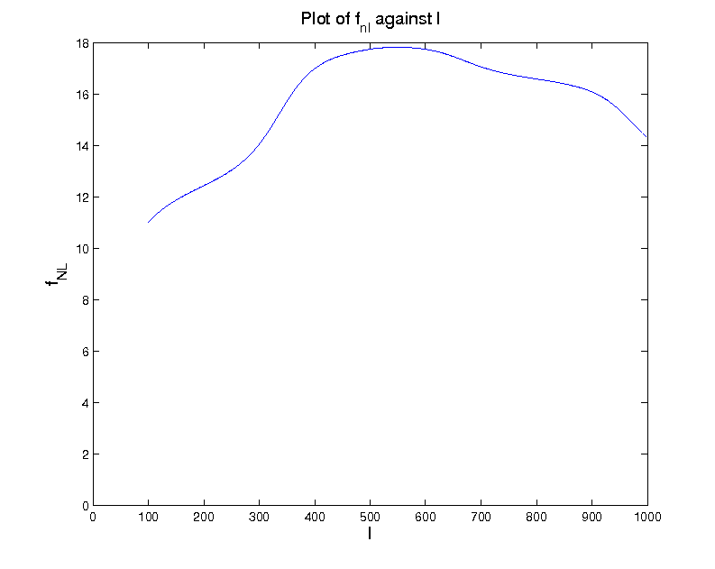
Refer to caption
Figure 2: Measure of the level of non-Gaussianity using fN​Llocalf_{NL}^{\mbox{local}}

IV.4 Numerical results

We have plotted the three dimensional bispectrum in the multipole range of Planck li<2000l_{i}<2000 by numerically integrating the analytic result (see Figures 3 and 4 ). In particular we plot the quantity (l1​l2​l3)4/3​B​(l1,l2,l3)(l_{1}l_{2}l_{3})^{4/3}B(l_{1},l_{2},l_{3}). We do not integrate out fully to the edge since the result begins to diverge there and is more difficult to evaluate numerically. We find that the signal peaks at around (500,500,500)(500,500,500) and drops towards the corners. Therefore, our assumption that using the equal ll values to estimate the level of non-Gaussianity seems valid. However, we do expect that the signal rises very near the edge (before it levels out) and so we use our approximations as detailed earlier to track this behaviour on slices across the bispectrum. In particular we show the slice for l1+l2+l3=2000l_{1}+l_{2}+l_{3}=2000 (Figure 5) and for l1+l2+l3=1500l_{1}+l_{2}+l_{3}=1500 (Figure 6). In order to see the behaviour more clearly we have multplied the bispectrum by a negative sign and we have shown the former plot as a contour lot. The slices are plotted in units of ϵ3=(8​π​G​μ)3\epsilon^{3}=(8\pi G\mu)^{3}. There is a peak towards the edge but only a factor of a few that at the centre point. Also it begins to diverge very near the edge for these slices. Therefore, we feel justified in neglecting the edges in our estimator for fN​Lf_{NL}.

Refer to caption
Figure 3: Plot of the 3D bispectrum (l1​l2​l3)4/3​B​(l1,l2,l3)(l_{1}l_{2}l_{3})^{4/3}B(l_{1},l_{2},l_{3}). The signal is seen to peak at the near the correlation length at last scattering for which all li≈500l_{i}\approx 500. Due to the resolution of the data points we do not pick up the rise towards the edge.
Refer to caption
Figure 4: Plot of the 3D bispectrum (l1​l2​l3)4/3​B​(l1,l2,l3)(l_{1}l_{2}l_{3})^{4/3}B(l_{1},l_{2},l_{3}) with difference slicings to that of Figure 3.
Refer to caption
Figure 5: Contour plot of the slice through the bispectrum at ∑ili=2000\sum_{i}l_{i}=2000.
Refer to caption
Figure 6: Plot of the slice through the bispectrum at ∑ili=1500\sum_{i}l_{i}=1500.

V Trispectrum

V.1 Trispectrum on small angular scales

As in the section on the bispectrum we regard kk as the angular multipole and ξ^\hat{\xi} to be the correlation length as measured at the original time (normalised by some factor as discussed previously). We will return the to the time dependence later in the calculation. However, we note here that as in the case for the power spectrum and bispectrum the total trispectrum reduces to the sum of equal time four point correlators between ts​t​a​r​t≳tl​s​st_{start}\gtrsim t_{lss} and t0t_{0}.

The trispectrum, in the flat sky approximation, is given (at any given time) by

⟨δ𝐤1​δ𝐤2​δ𝐤3​δ𝐤4⟩c=(2​π)2​δ(2)​(𝐤𝟏+𝐤𝟐+𝐤𝟑+𝐤𝟒)​Tc​(𝐤𝟏,𝐤𝟐,𝐤𝟑,𝐤𝟒)\displaystyle\left<\delta_{\mathbf{k}_{1}}\delta_{\mathbf{k}_{2}}\delta_{\mathbf{k}_{3}}\delta_{\mathbf{k}_{4}}\right>_{c}=(2\pi)^{2}\delta^{(2)}(\mathbf{k_{1}+k_{2}+k_{3}+k_{4}})T_{c}(\mathbf{k_{1},k_{2},k_{3},k_{4}})

where the subscript cc denotes the connected part. This suggest that we normalise the trispectrum by the area factor 𝒜\mathcal{A}. However, as we shall see below we should in fact normalise by 𝒜2\mathcal{A}^{2} for parallelogram configurations. The unconnected part, denoted hereafter by the subscript u​cuc, is given by

⟨δ𝐤1​δ𝐤2​δ𝐤3​δ𝐤4⟩u​c\displaystyle\left<\delta_{\mathbf{k}_{1}}\delta_{\mathbf{k}_{2}}\delta_{\mathbf{k}_{3}}\delta_{\mathbf{k}_{4}}\right>_{uc} =\displaystyle= (2​π)4​δ(2)​(𝐤𝟏+𝐤𝟐)​δ(2)​(𝐤𝟑+𝐤𝟒)​P​(k1)​P​(k3)+(2​π)4​δ(2)​(𝐤𝟏+𝐤𝟑)​δ(2)​(𝐤𝟐+𝐤𝟒)​P​(k1)​P​(k2)\displaystyle(2\pi)^{4}\delta^{(2)}(\mathbf{k_{1}+k_{2}})\delta^{(2)}(\mathbf{k_{3}+k_{4}})P(k_{1})P(k_{3})+(2\pi)^{4}\delta^{(2)}(\mathbf{k_{1}+k_{3}})\delta^{(2)}(\mathbf{k_{2}+k_{4}})P(k_{1})P(k_{2})
+(2​π)4​δ(2)​(𝐤𝟏+𝐤𝟒)​δ(2)​(𝐤𝟐+𝐤𝟑)​P​(k1)​P​(k2)\displaystyle+(2\pi)^{4}\delta^{(2)}(\mathbf{k_{1}+k_{4}})\delta^{(2)}(\mathbf{k_{2}+k_{3}})P(k_{1})P(k_{2})
=\displaystyle= 𝒜2​(δk1,k2​δk3,k4​P​(k1)​P​(k3)+δk1,k3​δk2,k4​P​(k1)​P​(k2)+δk1,k3​δk2,k4​P​(k1)​P​(k2))\displaystyle\mathcal{A}^{2}\left(\delta_{k_{1},k_{2}}\delta_{k_{3},k_{4}}P(k_{1})P(k_{3})+\delta_{k_{1},k_{3}}\delta_{k_{2},k_{4}}P(k_{1})P(k_{2})+\delta_{k_{1},k_{3}}\delta_{k_{2},k_{4}}P(k_{1})P(k_{2})\right)

We will calculate the four point correlator and subtract off this unconnected part to find the trispectrum.

In this paper we will consider only parallelogram configurations. In this regard we are motivated by the earlier section on the bispectrum which showed that as the triangle collapses it grows (though does not become infinite). Clearly, the parallelogram shape should replicate this behaviour.

For planar parallelograms (planar shapes are, of course, appropriate since we are using the flat sky approximation) we have that opposite sides are antiparallel. To impose this we need to use two delta functions and this implies that the trispectrum is normalised by 𝒜2\mathcal{A}^{2}. This is true in general, however, which becomes more apparent also when we note that we can decompose the delta via

δ(2)​(𝐤𝟏+𝐤𝟐+𝐤𝟑+𝐤𝟒)=∫d2​𝐋​δ(2)​(𝐤𝟏+𝐤𝟐+𝐋)​δ(2)​(𝐤𝟏+𝐤𝟐−𝐋).\displaystyle\delta^{(2)}(\mathbf{k_{1}+k_{2}+k_{3}+k_{4}})=\int d^{2}\mathbf{L}\delta^{(2)}(\mathbf{k_{1}+k_{2}+L})\delta^{(2)}(\mathbf{k_{1}+k_{2}-L}).

Then we infer that we can approximate the total trispectrum by summing over the possible parallelogram configurations (to specify a parallelogram configuration it suffices to have two of the sides and a diagonal)55 5 We shall see later in the section that the Gaussian contribution is given by square configurations..

Motivated by the above discussion we define

TT​(𝐤1,𝐤2,𝐤3,𝐤4)=1𝒜2​⟨δ𝐤1​δ𝐤2​δ𝐤3​δ𝐤4⟩\displaystyle T^{T}(\mathbf{k}_{1},\mathbf{k}_{2},\mathbf{k}_{3},\mathbf{k}_{4})=\frac{1}{\mathcal{A}^{2}}\left<\delta_{\mathbf{k}_{1}}\delta_{\mathbf{k}_{2}}\delta_{\mathbf{k}_{3}}\delta_{\mathbf{k}_{4}}\right>

where the multipoles trace out a parallelogram configuration.

In a similar fashion to the calculation of the power spectrum and bispectrum, we find that

TT​(𝐤1,𝐤2,𝐤3,𝐤4)=\displaystyle T^{T}(\mathbf{k}_{1},\mathbf{k}_{2},\mathbf{k}_{3},\mathbf{k}_{4})= (8​π​G​μ)4𝒜2​k1A​k2B​k3C​k4Dk12​k22​k32​k42​∫d​σ1​d​σ2​d​σ3​d​σ4​⟨X˙A​(σ1)​X˙B​(σ2)​X˙C​(σ3)​X˙D​(σ4)​ei​𝐤𝐚.𝐗𝐚⟩.\displaystyle\frac{(8\pi G\mu)^{4}}{\mathcal{A}^{2}}\frac{k_{1}^{A}k_{2}^{B}k_{3}^{C}k_{4}^{D}}{k_{1}^{2}k_{2}^{2}k_{3}^{2}k_{4}^{2}}\int d\sigma_{1}d\sigma_{2}d\sigma_{3}d\sigma_{4}\left<\dot{X}^{A}(\sigma_{1})\dot{X}^{B}(\sigma_{2})\dot{X}^{C}(\sigma_{3})\dot{X}^{D}(\sigma_{4})e^{i\mathbf{k_{a}.X_{a}}}\right>.

Writing CA​B​C​D=X˙A​(σ1)​X˙B​(σ2)​X˙C​(σ3)​X˙D​(σ4)C^{ABCD}=\dot{X}^{A}(\sigma_{1})\dot{X}^{B}(\sigma_{2})\dot{X}^{C}(\sigma_{3})\dot{X}^{D}(\sigma_{4}) and E=ka.XaE=k_{a}.X_{a} and using again the assumption of a Gaussian process we get that

⟨CA​B​C​D​ei​E⟩=⟨CA​B​C​D−12​CA​B​C​D​E2+124​CA​B​C​D​E4+…⟩\displaystyle\left<C^{ABCD}e^{iE}\right>=\left<C^{ABCD}-\frac{1}{2}C^{ABCD}E^{2}+\frac{1}{24}C^{ABCD}E^{4}+\dots\right>

Now

⟨CA​B​C​D⟩\displaystyle\left<C^{ABCD}\right> =\displaystyle= ⟨X˙1A​X˙2B​X˙3C​X˙4D⟩=δA​B2​V12​δC​D2​V34+δA​C2​V13​δB​D2​V24+δA​D2​V14​δB​C2​V23\displaystyle\left<\dot{X}^{A}_{1}\dot{X}^{B}_{2}\dot{X}^{C}_{3}\dot{X}^{D}_{4}\right>=\frac{\delta^{AB}}{2}V_{12}\frac{\delta^{CD}}{2}V_{34}+\frac{\delta^{AC}}{2}V_{13}\frac{\delta^{BD}}{2}V_{24}+\frac{\delta^{AD}}{2}V_{14}\frac{\delta^{BC}}{2}V_{23}
⟹k1A​k2B​k3C​k4D​⟨CA​B​C​D⟩\displaystyle\implies k_{1}^{A}k_{2}^{B}k_{3}^{C}k_{4}^{D}\left<C^{ABCD}\right> =\displaystyle= 14​(κ12​κ34​V12​V34+κ13​κ24​V13​V24+κ14​κ23​V14​V23)\displaystyle\frac{1}{4}\left(\kappa_{12}\kappa_{34}V_{12}V_{34}+\kappa_{13}\kappa_{24}V_{13}V_{24}+\kappa_{14}\kappa_{23}V_{14}V_{23}\right)

Next we consider (writing CA​B​C​DC^{ABCD} as A​B​C​DABCD)

⟨A​B​C​D​E2⟩=\displaystyle\left<ABCDE^{2}\right>= ⟨CA​B​C​D⟩​⟨E2⟩+2​⟨A​B⟩​⟨C​E⟩​⟨D​E⟩+↺\displaystyle\left<C^{ABCD}\right>\left<E^{2}\right>+2\left<AB\right>\left<CE\right>\left<DE\right>+\circlearrowleft

where ↺\circlearrowleft denotes the contribution from terms found by permutating the symbols A,B,C,DA,B,C,D in the the second term on the right hand side of the equality66 6 We note that the factor of two appears since ⟨A​B⟩=⟨B​A⟩\left<AB\right>=\left<BA\right>.. Now we note that (using ∑i𝐤i=0\sum_{i}\mathbf{k}_{i}=0)

⟨A​B⟩​⟨C​E⟩​⟨D​E⟩\displaystyle\left<AB\right>\left<CE\right>\left<DE\right> =\displaystyle= δA​B​V122​⟨X˙3C​∑j≠3kjE​Xj​3E⟩​⟨X˙4D​∑j≠4kjE​Xj​4E⟩\displaystyle\frac{\delta^{AB}V_{12}}{2}\left<\dot{X}^{C}_{3}\sum_{j\neq 3}k_{j}^{E}X_{j3}^{E}\right>\left<\dot{X}^{D}_{4}\sum_{j\neq 4}k_{j}^{E}X_{j4}^{E}\right>
=\displaystyle= δA​B​V128​∑j≠3kjC​Π3​j​∑j≠4kjD​Π4​j\displaystyle\frac{\delta^{AB}V_{12}}{8}\sum_{j\neq 3}k_{j}^{C}\Pi_{3j}\sum_{j\neq 4}k_{j}^{D}\Pi_{4j}

where we use the fact that Πi​j=⟨Xi​jAX˙jA⟩=−<X˙jAXj​iA>\Pi_{ij}=\left<X^{A}_{ij}\dot{X}_{j}^{A}\right>=-<\dot{X}_{j}^{A}X^{A}_{ji}>. Suppressing the summation notation we find that

k1A​k2B​k3C​k4D​⟨A​B​C​D​E2⟩=⟨CA​B​C​D⟩​⟨E2⟩+\displaystyle k_{1}^{A}k_{2}^{B}k_{3}^{C}k_{4}^{D}\left<ABCDE^{2}\right>=\left<C^{ABCD}\right>\left<E^{2}\right>+
14​(V12​κ12​κ3​j​Π3​j​κ4​j​Π4​j+V13​κ13​κ2​j​Π2​j​κ4​j​Π4​j+V14​κ14​κ2​j​Π2​j​κ3​j​Π3​j)+\displaystyle\frac{1}{4}\left(V_{12}\kappa_{12}\kappa_{3j}\Pi_{3j}\kappa_{4j}\Pi_{4j}+V_{13}\kappa_{13}\kappa_{2j}\Pi_{2j}\kappa_{4j}\Pi_{4j}+V_{14}\kappa_{14}\kappa_{2j}\Pi_{2j}\kappa_{3j}\Pi_{3j}\right)+
14​(V23​κ23​κ1​j​Π1​j​κ4​j​Π4​j+V24​κ24​κ1​j​Π1​j​κ3​j​Π3​j+V34​κ34​κ1​j​Π1​j​κ3​j​Π3​j).\displaystyle\frac{1}{4}\left(V_{23}\kappa_{23}\kappa_{1j}\Pi_{1j}\kappa_{4j}\Pi_{4j}+V_{24}\kappa_{24}\kappa_{1j}\Pi_{1j}\kappa_{3j}\Pi_{3j}+V_{34}\kappa_{34}\kappa_{1j}\Pi_{1j}\kappa_{3j}\Pi_{3j}\right).

Now we proceed to investigate

⟨A​B​C​D​E4⟩=\displaystyle\left<ABCDE^{4}\right>= ⟨A​B​C​D​E2⟩​⟨E2⟩+24​⟨A​E⟩​⟨B​E⟩​⟨C​E⟩​⟨D​E⟩.\displaystyle\left<ABCDE^{2}\right>\left<E^{2}\right>+24\left<AE\right>\left<BE\right>\left<CE\right>\left<DE\right>.

We have seen above that ⟨AE⟩=−12∑j≠1kjAΠ1​j\left<AE\right>=-\dfrac{1}{2}\sum_{j\neq 1}k_{j}^{A}\Pi_{1j} so (again suppressing the summation notation) we have

k1A​k2B​k3C​k4D​⟨A​E⟩​⟨B​E⟩​⟨C​E⟩​⟨D​E⟩=2416​κ1​j​Π1​j​κ2​j​Π2​j​κ3​j​Π3​j​κ4​j​Π4​j\displaystyle k_{1}^{A}k_{2}^{B}k_{3}^{C}k_{4}^{D}\left<AE\right>\left<BE\right>\left<CE\right>\left<DE\right>=\frac{24}{16}\kappa_{1j}\Pi_{1j}\kappa_{2j}\Pi_{2j}\kappa_{3j}\Pi_{3j}\kappa_{4j}\Pi_{4j}

Finally, we collect the terms to find that

k1A​k2B​k3C​k4D​⟨CA​B​C​D​ei​E⟩\displaystyle k_{1}^{A}k_{2}^{B}k_{3}^{C}k_{4}^{D}\left<C^{ABCD}e^{iE}\right> =\displaystyle= [14(κ12κ34V12V34+κ13κ24V13V24κ14κ23V14V23)\displaystyle[\frac{1}{4}\left(\kappa_{12}\kappa_{34}V_{12}V_{34}+\kappa_{13}\kappa_{24}V_{13}V_{24}\kappa_{14}\kappa_{23}V_{14}V_{23}\right)
−18(V12κ12κ3​jΠ3​jκ4​jΠ4​j+↺)+116κ1​jΠ1​jκ2​jΠ2​jκ3​jΠ3​jκ4​jΠ4​j]e−⟨E2⟩/2\displaystyle-\frac{1}{8}\left(V_{12}\kappa_{12}\kappa_{3j}\Pi_{3j}\kappa_{4j}\Pi_{4j}+\circlearrowleft\right)+\frac{1}{16}\kappa_{1j}\Pi_{1j}\kappa_{2j}\Pi_{2j}\kappa_{3j}\Pi_{3j}\kappa_{4j}\Pi_{4j}]e^{-\left<E^{2}\right>/2}

where we have

⟨E2⟩\displaystyle\left<E^{2}\right> =\displaystyle= ⟨(k1A​X14A+k2A​X24A+k3A​X34A)​(k2B​X21B+k3B​X31B+k4B​X41B)⟩\displaystyle\left<(k_{1}^{A}X_{14}^{A}+k_{2}^{A}X_{24}^{A}+k_{3}^{A}X_{34}^{A})(k_{2}^{B}X_{21}^{B}+k_{3}^{B}X_{31}^{B}+k_{4}^{B}X_{41}^{B})\right>
=\displaystyle= −12​(κ12​Γ12+κ13​Γ13+κ14​Γ14+κ23​Γ23+κ24​Γ24+κ34​Γ34)\displaystyle-\frac{1}{2}\left(\kappa_{12}\Gamma_{12}+\kappa_{13}\Gamma_{13}+\kappa_{14}\Gamma_{14}+\kappa_{23}\Gamma_{23}+\kappa_{24}\Gamma_{24}+\kappa_{34}\Gamma_{34}\right)

and where we use the notation ↺\circlearrowleft to represent the non-equivalent contributions by permuting the symbols (1,2,3,4)(1,2,3,4) of the term in the brackets. The dominant term on all angular scales is found to be given by the first term (∼CA​B​C​De−E2/2\sim C^{ABCD}e^{-E^{2}/2}) and, therefore, in what follows we neglect the remaining terms.

For a parallelogram configuration we have κ13=−k12,κ24=−k22,κ23=κ14=−κ34=−κ12\kappa_{13}=-k_{1}^{2},\,\kappa_{24}=-k_{2}^{2},\,\kappa_{23}=\kappa_{14}=-\kappa_{34}=-\kappa_{12}. This implies that, in the small angle approximation,

⟨E2⟩\displaystyle\left<E^{2}\right> =\displaystyle= −t¯22​(κ12​σ122−k12​Γ13−κ12​σ142−κ12​σ232−k22​σ242+κ12​σ342)\displaystyle\frac{-\overline{t}^{2}}{2}\left(\kappa_{12}\sigma_{12}^{2}-k_{1}^{2}\Gamma_{13}-\kappa_{12}\sigma_{14}^{2}-\kappa_{12}\sigma_{23}^{2}-k_{2}^{2}\sigma_{24}^{2}+\kappa_{12}\sigma_{34}^{2}\right)

Again the choice of independent variables is dependent on the integrand under consideration. To elucidate this we consider the term

∫dσ1dσ2dσ3dσ4V13V24exp(−E2/2)=ℒ8∫dσ12dσ13dσ24V13Π12exp(−E2/2)\displaystyle\int d\sigma_{1}d\sigma_{2}d\sigma_{3}d\sigma_{4}V_{13}V_{24}\exp(-E^{2}/2)=\frac{\mathcal{L}}{8}\int d\sigma_{12}d\sigma_{13}d\sigma_{24}V_{13}\Pi_{12}\exp(-E^{2}/2)

In a similar manner to the case of the bispectrum we can simplify the calculation by making a separable approximation. In particular we find

exp(−⟨E2⟩/2)\displaystyle\exp(-\left<E^{2}\right>/2) =\displaystyle= exp⁡(t¯24​(κ12​σ122−k12​Γ13−κ12​σ142−κ12​σ232−k22​σ242+κ12​σ342))\displaystyle\exp\left(\frac{\overline{t}^{2}}{4}\left(\kappa_{12}\sigma_{12}^{2}-k_{1}^{2}\Gamma_{13}-\kappa_{12}\sigma_{14}^{2}-\kappa_{12}\sigma_{23}^{2}-k_{2}^{2}\sigma_{24}^{2}+\kappa_{12}\sigma_{34}^{2}\right)\right)
=\displaystyle= OPENexp⁡(−t¯24​((k1​σ13−κ12k1​σ23)2+k12​k22−κ122k12​σ242)))\displaystyle\exp\left(-\frac{\overline{t}^{2}}{4}\left((k_{1}\sigma_{13}-\frac{\kappa_{12}}{k_{1}}\sigma_{23})^{2}+\frac{k_{1}^{2}k_{2}^{2}-\kappa_{12}^{2}}{k_{1}^{2}}\sigma_{24}^{2})\right)\right)
∫dσ1dσ2dσ3dσ4V13V24exp(−E2/2)=ℒ24∫dσ13V13exp(−k12​t¯2​σ1324)∫dσ24V24exp(−K12​t¯2​σ2424)\displaystyle\int d\sigma_{1}d\sigma_{2}d\sigma_{3}d\sigma_{4}V_{13}V_{24}\exp(-E^{2}/2)=\frac{\mathcal{L}^{2}}{4}\int d\sigma_{13}V_{13}\exp\left(-\frac{k_{1}^{2}\overline{t}^{2}\sigma_{13}^{2}}{4}\right)\int d\sigma_{24}V_{24}\exp\left(-\frac{K_{1}^{2}\overline{t}^{2}\sigma_{24}^{2}}{4}\right)

where Ki=2​Area△/kiK_{i}=2\mbox{Area}_{\triangle}/k_{i} as defined in the section on the bispectrum (note that the area of the triangle is half that of the parallelogram). Since K2K_{2} (divided by t0t_{0}) may be less than 500500, i.e. correspond to an angular scale below that of the correlation length then we should use a better approximation to V24V_{24}. Following these approximations for all terms and using the results of the previous sections we find that

TT(𝐤1,𝐤2,𝐤3,𝐤4)≈ℒ2​ξ^2𝒜2(8​π​G​μ)4ξ^2​k12​k22​k32​k42116(∫dσ12dσ342κ122V12V34exp(−E2/2)+∫dσ13dσ24k12k22V13V24exp(−E2/2))\displaystyle T^{T}(\mathbf{k}_{1},\mathbf{k}_{2},\mathbf{k}_{3},\mathbf{k}_{4})\approx\frac{\mathcal{L}^{2}\hat{\xi}^{2}}{\mathcal{A}^{2}}\frac{(8\pi G\mu)^{4}}{\hat{\xi}^{2}k_{1}^{2}k_{2}^{2}k_{3}^{2}k_{4}^{2}}\frac{1}{16}\left(\int d\sigma_{12}d\sigma_{34}2\kappa_{12}^{2}V_{12}V_{34}\exp(-E^{2}/2)+\int d\sigma_{13}d\sigma_{24}k_{1}^{2}k_{2}^{2}V_{13}V_{24}\exp(-E^{2}/2)\right)

We note also that in the case of a square this gives P⁡(k1)​P​(k2)P(k_{1})P(k_{2}) at each time. This is the Gaussian contribution. Therefore the approximation to the total trispectrum is given by the sum over non-square parallelogram configurations. In order to compute the integral we use the more accurate approximation for VV. Using the previous expressions for the separate integrals we find

TT​(𝐤1,𝐤2,𝐤3,𝐤4)≈ℒ2​ξ^2𝒜2​(8​π​G​μ)4ξ^2​k12​k22​k32​k42​v¯44​1t¯6​ξ^4​Area3​(2​κ122​f2​(K2​ξ^2)​f2​(k2​ξ^)+k12​k22​f2​(K1​ξ^)​f2​(k1​ξ^))\displaystyle T^{T}(\mathbf{k}_{1},\mathbf{k}_{2},\mathbf{k}_{3},\mathbf{k}_{4})\approx\frac{\mathcal{L}^{2}\hat{\xi}^{2}}{\mathcal{A}^{2}}\frac{(8\pi G\mu)^{4}}{\hat{\xi}^{2}k_{1}^{2}k_{2}^{2}k_{3}^{2}k_{4}^{2}}\frac{\overline{v}^{4}}{4}\frac{1}{\overline{t}^{6}\hat{\xi}^{4}\mbox{Area}^{3}}\left(2\kappa_{12}^{2}f_{2}(K_{2}\hat{\xi}^{2})f_{2}(k_{2}\hat{\xi})+k_{1}^{2}k_{2}^{2}f_{2}(K_{1}\hat{\xi})f_{2}(k_{1}\hat{\xi})\right)

where Area=2​Area△\mbox{Area}=2\mbox{Area}_{\triangle}.

This result must be integrated as usual to give the total trispectrum due to cosmic strings between last scattering (or if km<500k_{m}<500 between ts​t​a​r​t=tl​s​s​500/kmt_{start}=t_{lss}500/k_{m}) and today. Returning the time dependence using the renormalised time t/ts​t​a​r​tt/t_{start} and understanding the multipoles to refer to angular multipoles we have that the total trispectrum contribution by the parallelogram considered here is

Tt​o​t​a​l​(𝐤1,𝐤2,𝐤3,𝐤4)≈\displaystyle T^{total}(\mathbf{k}_{1},\mathbf{k}_{2},\mathbf{k}_{3},\mathbf{k}_{4})\approx ℒ2​ξ^2𝒜2​(8​π​G​μ)4ξ~2​k12​k22​k32​k42​v¯44​1t¯6​ξ~4​Area3\displaystyle\frac{\mathcal{L}^{2}\hat{\xi}^{2}}{\mathcal{A}^{2}}\frac{(8\pi G\mu)^{4}}{\tilde{\xi}^{2}k_{1}^{2}k_{2}^{2}k_{3}^{2}k_{4}^{2}}\frac{\overline{v}^{4}}{4}\frac{1}{\overline{t}^{6}\tilde{\xi}^{4}\mbox{Area}^{3}}
∫1t0/tl​s​sd​t​1t6​(2​κ122​f2​(K2​ξ~​t)​f2​(k2​ξ~​t)+k12​k22​f2​(K1​ξ~​t)​f2​(k1​ξ~​t))\displaystyle\int_{1}^{t_{0}/t_{lss}}dt\frac{1}{t^{6}}\left(2\kappa_{12}^{2}f_{2}(K_{2}\tilde{\xi}t)f_{2}(k_{2}\tilde{\xi}t)+k_{1}^{2}k_{2}^{2}f_{2}(K_{1}\tilde{\xi}t)f_{2}(k_{1}\tilde{\xi}t)\right)

In order to understand the behaviour for the trispectrum we note the following approximation to the integral given by

Tt​o​t​a​l​(𝐤1,𝐤2,𝐤3,𝐤4)≈\displaystyle T^{total}(\mathbf{k}_{1},\mathbf{k}_{2},\mathbf{k}_{3},\mathbf{k}_{4})\approx ℒ2​ξ^2𝒜2​(8​π​G​μ)4ξ~2​k12​k22​k32​k42​v¯44​πt¯2​Area\displaystyle\frac{\mathcal{L}^{2}\hat{\xi}^{2}}{\mathcal{A}^{2}}\frac{(8\pi G\mu)^{4}}{\tilde{\xi}^{2}k_{1}^{2}k_{2}^{2}k_{3}^{2}k_{4}^{2}}\frac{\overline{v}^{4}}{4}\frac{\pi}{\overline{t}^{2}\mbox{Area}}
(2​κ122​erfc​(1ξ~​k2​t¯)​exp⁡(1(ξ~​k2​t¯)2)​erfc​(1ξ~​K2​t¯)​exp⁡(1(ξ~​K2​t¯)2)CLOSE\displaystyle(2\kappa_{12}^{2}\mbox{erfc}\left(\frac{1}{\tilde{\xi}k_{2}\overline{t}}\right)\exp\left(\frac{1}{(\tilde{\xi}k_{2}\overline{t})^{2}}\right)\mbox{erfc}\left(\frac{1}{\tilde{\xi}K_{2}\overline{t}}\right)\exp\left(\frac{1}{(\tilde{\xi}K_{2}\overline{t})^{2}}\right)
OPEN+k12​k22​erfc​(1ξ~​k1​t¯)​exp⁡(1(ξ~​k1​t¯)2)​erfc​(1ξ~​K1​t¯)​exp⁡(1(ξ~​K1​t¯)2)).\displaystyle+k_{1}^{2}k_{2}^{2}\mbox{erfc}\left(\frac{1}{\tilde{\xi}k_{1}\overline{t}}\right)\exp\left(\frac{1}{(\tilde{\xi}k_{1}\overline{t})^{2}}\right)\mbox{erfc}\left(\frac{1}{\tilde{\xi}K_{1}\overline{t}}\right)\exp\left(\frac{1}{(\tilde{\xi}K_{1}\overline{t})^{2}}\right)).

Using the asymptotic expansion of erfc we find that as K→0K\rightarrow 0 the formula is independent of KK, i.e. of Area. Therefore, as for the bispectrum, the trispectrum grows towards the edge but is not divergent (i.e. it reaches a cutoff).

V.2 Trispectrum on large angular scales

If min⁡ki=km≲500\min k_{i}=k_{m}\lesssim 500, then we must restrict the range of times over which we sum to (ts​t​a​r​t,t0)(t_{start},t_{0}). Again we find that the trispectrum decreases as a logarithm as we restrict the range, i.e. the trispectrum ∝ln⁡((km/500)​t0/tl​s​s)≈ln⁡(km/10)\propto\ln((k_{m}/500)t_{0}/t_{lss})\approx\ln(k_{m}/10). Therefore, we can include this effect by multiplying the formulae in the previous section by ln⁡(km/10)/ln⁡(50)\ln(k_{m}/10)/\ln(50) for km≲500k_{m}\lesssim 500. This is the same effect as was evident in the case of the bispectrum and the power spectrum. That we can extend the range of multipoles to less than 500500 means that we can use this formalism to make a prediction for τN​L\tau_{NL} generated by cosmic strings in the multipole range of Planck.

V.3 Estimator of τN​L\tau_{NL}

The signal to noise ratio for the trispectrum (assuming the noise is cosmic variance dominated) is given by

(S/N)2=∑l1≤l2≤l3≤l4∑L|Tl1​l2​l3​l4​(L)|2(2​L+1)​Cl1​Cl2​Cl3​Cl4=124​∑l1,l2,l3,l4∑L|Tl1​l2​l3​l4​(L)|2(2​L+1)​Cl1​Cl2​Cl3​Cl4\displaystyle(S/N)^{2}=\sum_{l_{1}\leq l_{2}\leq l_{3}\leq l_{4}}\sum_{L}\frac{|T_{l_{1}l_{2}l_{3}l_{4}}(L)|^{2}}{(2L+1)C_{l_{1}}C_{l_{2}}C_{l_{3}}C_{l_{4}}}=\frac{1}{24}\sum_{l_{1},l_{2},l_{3},l_{4}}\sum_{L}\frac{|T_{l_{1}l_{2}l_{3}l_{4}}(L)|^{2}}{(2L+1)C_{l_{1}}C_{l_{2}}C_{l_{3}}C_{l_{4}}}

where Tl1​l2​l3​l4​(L)T_{l_{1}l_{2}l_{3}l_{4}}(L) is one of the possible configurations of the full-sky trispectrum. In order to find the signal to noise ratio we therefore must relate the full sky trispectrum to the flat sky equivlaent ([20]).

Decomposing the temperature perturbation in terms of spherical harmonics we have

Δ​TT​(𝐧^)=al​m​Yl​m​(𝐧^).\displaystyle\frac{\Delta T}{T}(\mathbf{\hat{n}})=a_{lm}Y_{lm}(\mathbf{\hat{n}}).

In the flat sky limit the temperature perturbation is expressed in terms of Fourier harmonics

Δ​TT​(𝐧^)=∫d2​l(2​π)2​δ​(𝐥𝟏)​ei​𝐥.𝐧^.\displaystyle\frac{\Delta T}{T}(\mathbf{\hat{n}})=\int\frac{d^{2}l}{(2\pi)^{2}}\delta(\mathbf{l_{1}})e^{i\mathbf{l.\hat{n}}}.

The relationship between the full-sky and flat-sky limit is obtained by noting

al​m\displaystyle a_{lm} =\displaystyle= im​2​l+14​π​∫d​ϕl2​π​ei​m​ϕl​δ​(𝐥),\displaystyle i^{m}\sqrt{\frac{2l+1}{4\pi}}\int\frac{d\phi_{l}}{2\pi}e^{im\phi_{l}}\delta(\mathbf{l}),
δ⁡(𝐥𝟏+𝐥𝟐+𝐥𝟑+𝐥𝟒)\displaystyle\delta(\mathbf{l_{1}+l_{2}+l_{3}+l_{4}}) =\displaystyle= ∫d​𝐧^(2​π)2​ei⁡(𝐥𝟏+𝐥𝟐+𝐥𝟑+𝐥𝟒).𝐧^\displaystyle\int\frac{d\mathbf{\hat{n}}}{(2\pi)^{2}}e^{i(\mathbf{l_{1}+l_{2}+l_{3}+l_{4}}).\mathbf{\hat{n}}}
ei​𝐥,𝐧^\displaystyle e^{i\mathbf{l,\hat{n}}} =\displaystyle= 2​πl​∑mim​Yl​m​(𝐧^)​ei​m​ϕl\displaystyle\frac{2\pi}{l}\sum_{m}i^{m}Y_{lm}(\mathbf{\hat{n}})e^{im\phi_{l}}
⟨al1​m1​al2​m2​al3​m3​al4​m4⟩c\displaystyle\left<a_{l_{1}m_{1}}a_{l_{2}m_{2}}a_{l_{3}m_{3}}a_{l_{4}m_{4}}\right>_{c} =\displaystyle= (Πi=14​li2​π​e−i​mi​ϕli)​(2​π)2​δ​(𝐥𝟏+𝐥𝟐+𝐥𝟑+𝐥𝟒)​T(l3,l4)(l1,l2)\displaystyle\left(\Pi_{i=1}^{4}\sqrt{\frac{l_{i}}{2\pi}}e^{-im_{i}\phi_{l_{i}}}\right)(2\pi)^{2}\delta(\mathbf{l_{1}+l_{2}+l_{3}+l_{4}})T^{(l_{1},l_{2})}_{(l_{3},l_{4})}

where ϕl\phi_{l} denotes the polar angle of 𝐥\mathbf{l} and T(l3,l4)(l1,l2)T^{(l_{1},l_{2})}_{(l_{3},l_{4})} denotes the flat sky trispectrum given by a configuration with multipoles l1,l2,l3,l4l_{1},l_{2},l_{3},l_{4} (and where l12l_{12} is the diagonal of the quadrilateral that makes a triangle with l1,l2l_{1},l_{2}). Using these formulae we find

δ⁡((𝐥𝟏+𝐥𝟐+𝐥𝟑+𝐥𝟒))\displaystyle\delta((\mathbf{l_{1}+l_{2}+l_{3}+l_{4}})) =\displaystyle= ∫d2​L​δ​((𝐥𝟏+𝐥𝟐+𝐋))​δ​((𝐥𝟑+𝐥𝟒−𝐋))\displaystyle\int d^{2}L\delta((\mathbf{l_{1}+l_{2}+L}))\delta((\mathbf{l_{3}+l_{4}-L}))
=\displaystyle= 1(2​π)2∑mi∑L,M(Πi=142​πliei​mi​ϕli)2​L+14​π×\displaystyle\frac{1}{(2\pi)^{2}}\sum_{m_{i}}\sum_{L,M}\left(\Pi_{i=1}^{4}\sqrt{\frac{2\pi}{l_{i}}}e^{im_{i}\phi_{l_{i}}}\right)\frac{2L+1}{4\pi}\times
(2​l1+1)​(2​l2+1)​(2​l3+1)​(2​l4+1)(l1l2L000)(l3l4L000)×\displaystyle\sqrt{(2l_{1}+1)(2l_{2}+1)(2l_{3}+1)(2l_{4}+1)}\left(\begin{array}[]{ccc}l_{1}&l_{2}&L\\ 0&0&0\end{array}\right)\left(\begin{array}[]{ccc}l_{3}&l_{4}&L\\ 0&0&0\end{array}\right)\times
(−1)M​(l1l2Lm1m2M)​(l3l4Lm3m4−M).\displaystyle(-1)^{M}\left(\begin{array}[]{ccc}l_{1}&l_{2}&L\\ m_{1}&m_{2}&M\end{array}\right)\left(\begin{array}[]{ccc}l_{3}&l_{4}&L\\ m_{3}&m_{4}&-M\end{array}\right).

Combining these results we can write the full sky trispectrum in terms of the flat sky trispectrum as

Tl1​l2​l3​l4​(L)=2​L+14​π​(2​l1+1)​(2​l2+1)​(2​l3+1)​(2​l4+1)​(l1l2L000)​(l3l4L000)​T(l3​l4)(l1​l2)​(L).\displaystyle T_{l_{1}l_{2}l_{3}l_{4}}(L)=\frac{2L+1}{4\pi}\sqrt{(2l_{1}+1)(2l_{2}+1)(2l_{3}+1)(2l_{4}+1)}\left(\begin{array}[]{ccc}l_{1}&l_{2}&L\\ 0&0&0\end{array}\right)\left(\begin{array}[]{ccc}l_{3}&l_{4}&L\\ 0&0&0\end{array}\right)T^{(l_{1}l_{2})}_{(l_{3}l_{4})}(L).

With this consideration we can make an estimate of the signal to noise ratio for the trispectrum. We note also that we need only consider even terms since the Wigner-3​j3j vanishes for li+lj+Li​j=oddl_{i}+l_{j}+L_{ij}=\mbox{odd}.

We are interested in finding an estimate for τN​L\tau_{NL}. We note that for the local model of inflation, [21] (for which τN​L=(6​fN​L/5)2\tau_{NL}=(6f_{NL}/5)^{2}), the signal to noise ratio is given approximately by

(S/N)l​o​c​a​l≈5×10−18​fN​L4​(l​o​c​a​l)​lm​a​x4≈2.4×10−18​τN​L2​(l​o​c​a​l)​lm​a​x4\displaystyle(S/N)^{local}\approx 5\times 10^{-18}f_{NL}^{4(local)}l_{max}^{4}\approx 2.4\times 10^{-18}\tau_{NL}^{2(local)}l_{max}^{4}

Observationally the trispectrum has not received much attention with the rather weak constraint τN​L<108\tau_{NL}<10^{8} [whomever]. Recently there has been a significant improvement claimed using N-point probability distributions [22] with −5.6×10⁵<τN​L<6.4×10⁵-5.6\times 10^{5}<\tau_{NL}<6.4\times 10^{5}. Again these results are for a local-type non-Gaussianity which is unlike the less peaked cosmic string trispectrum, so a more specific analysis will be necessary to achieve quantitative constraints.

VI Conclusions

In this paper, we have endeavoured to analytically calculate the cosmic string power spectrum, bispectrum and trispectrum over a range of scales relevant for CMB experiments on both large and small angular scales. We have been particularly focused on extending previous work to multipole ranges (l<2000l<2000) applicable for the Planck satellite, an experiment which has the potential to dramatically improve constraints on all these correlators. We have presented a relatively featureless shape for the bispectrum over the relevant range which should be easily distinguishable from the oscillatory peaks of inflationary bispectra [8] if there is a significant signal discovered. Our preliminary estimates of fN​Lf_{NL} from cosmic strings indicate that Planck constraints from the bispectrum should be competitive with those from the power spectrum. We note that we obtain a considerably smaller estimate than the fN​L=−1000f_{NL}=-1000 in ref. [11] for several reasons, including the extension of our analysis over lower multipole ranges relevant for WMAP, a more careful comparison with fN​Lf_{NL} estimators used in the literature, and a lower normalisation of the string spectrum derived for Nambu strings [5], rather than that obtained from field theory simulations [6]. Nevertheless, as we shall discuss, our estimate contains many uncertainties and more detailed and accurate forecasts are the subject of ongoing work [12].

We have also evaluated the CMB trispectrum (for parallelogram configurations) on the relevant multipole scales for WMAP and Planck. Again we find a relatively constant trispectrum, finite in all regimes and for which we do not expect dramatic features for other configurations. Our results indicate a relatively larger signature for the trispectrum, in contrast to the amplitude of the bispectrum which is suppressed because it depends on the poor correlation between the string velocity and curvature. Our preliminary estimate of τN​L\tau_{NL} a few times 10410^{4} needs a more detailed analysis to characterise key uncertainties more carefully. Nevertheless, the trispectrum deserves much closer scrutiny observationally and the prospect of constraining cosmic strings should motivate the development of suitable estimators.

These analytic calculations of the post-recombination gravitational effects of cosmic strings offer important physical insights into the CMB correlations they induce. However, we note that there are many directions in which they can be substantially improved. Detailed numerical investigations of the CMB power spectrum created by cosmic strings and other topological defects already takes into account a far wider range of physical effects, notably recombination physics around decoupling and a better description of the evolving string network. It should be possible to similarly develop the unequal time correlation methods presented for the late time GKS signatures here to calculate both the bispectrum and the trispectrum to high accuracy numerically. In the meantime, however, it is a matter of comparing the present analytic results with CMB maps induced by cosmic string networks on both large (full sky) and small scales in order to get a more accurate normalisation and characterisation of the bispectrum and trispectrum. Given the stark contrast between the string shapes with those predicted by inflation, there needs also to be a specific search for these signatures in present and forthcoming CMB data, a project which is being actively investigated [12]. There seem to be good prospects of using forthcoming CMB data to obtain new insight into cosmic string scenarios using higher order correlators.

VII Acknowledgements

We are very grateful for many informative discussions with James Fergusson and also for generating the three dimensional bispectrum images. We also acknowledge useful conversations with David Seery and Michele Liguori. EPS was supported by STFC grant ST/F002998/1 and the Centre for Theoretical Cosmology. DMR was supported by EPSRC, the Isaac Newton Trust and the Cambridge European Trust. We are grateful for the hospitality of the Tufts Taillores Centre during the Vilenkinfest in September 2009 where these results were first reported.

Note added in proof: While this manuscript was nearing completion, related results for the string trispectrum were presented in [23].

References

  • [1] G. Dvali and S. H. H. Tye. Brane inflation. Phys. Lett., B450:72, 1999.
  • [2] R. Jeannerot, J. Rocher, and M. Sakellariadou. How generic is cosmic string formation in susy guts. Phys. Rev., D68:103514, 2003.
  • [3] J. Richard Gott. Gravitational lensing effects of vacuum strings: Exact solutions. Astrophys. J., 288:422–427, 1985.
  • [4] Nick Kaiser and A. Stebbins. Microwave Anisotropy Due to Cosmic Strings. Nature, 310:391–393, 1984.
  • [5] Richard A. Battye, Bjorn Garbrecht, and Apostolos Pilaftsis. Textures and Semi-Local Strings in SUSY Hybrid Inflation. JCAP, 0809:020, 2008.
  • [6] Jon Urrestilla, Neil Bevis, Mark Hindmarsh, Martin Kunz, and Andrew R. Liddle. Cosmic microwave anisotropies from BPS semilocal strings. JCAP, 0807:010, 2008.
  • [7] Juan Martin Maldacena. Non-Gaussian features of primordial fluctuations in single field inflationary models. JHEP, 05:013, 2003.
  • [8] J. R. Fergusson and E. P. S. Shellard. The shape of primordial non-gaussianity and the cmb bispectrum. Physical Review D, 80:043510, 2009.
  • [9] Xingang Chen, Min-xin Huang, Shamit Kachru, and Gary Shiu. Observational signatures and non-Gaussianities of general single field inflation. JCAP, 0701:002, 2007.
  • [10] Mark Hindmarsh, Christophe Ringeval, and Teruaki Suyama. The cmb temperature trispectrum of cosmic strings, 2009.
  • [11] M. Hindmarsh. Small scale microwave background fluctuations from cosmic strings. Astrophysics Journal, 431:534–542, 1994.
  • [12] J. R. Fergusson, E. P. S. Shellard, M.Landriau, D. M. Regan, and M. Liguori. In preparation.
  • [13] A. Stebbins. Cosmic strings and the microwave sky. I - Anisotropy from moving strings. Astrophys. J. , 327:584–614, April 1988.
  • [14] C. J. A. P. Martins and E. P. S. Shellard. Quantitative string evolution. Phys. Rev., D54:2535–2556, 1996.
  • [15] Levon Pogosian and Tanmay Vachaspati. Cosmic microwave background anisotropy from wiggly strings. Phys. Rev., D60:083504, 1999.
  • [16] Daniel Babich and Matias Zaldarriaga. Primordial bispectrum information from cmb polarization. Physical Review D, 70:083005, 2004.
  • [17] F.R. Bouchet D.P. Bennett, A. Stebbins. The implications of the cobe-dmr results for cosmic strings. Astrophysics Journal, 399:L5–L8, 1992.
  • [18] B. Allen and E. P. S. Shellard. Cosmic string evolution: A numerical simulation. Phys. Rev. Lett., 64:119–122, 1990.
  • [19] Leonardo Senatore, Kendrick M. Smith, and Matias Zaldarriaga. Non-gaussianities in single field inflation and their optimal limits from the wmap 5-year data, 2009.
  • [20] Wayne Hu. The angular trispectrum of the cmb. Physical Review D, 64:083005, 2001.
  • [21] Noriyuki Kogo and Eiichiro Komatsu. Angular trispectrum of cmb temperature anisotropy from primordial non-gaussianity with the full radiation transfer function. Physical Review D, 73:083007, 2006.
  • [22] P. Vielva and J. L. Sanz. Constraints on f_nl and g_nl from the analysis of the n-pdf of the cmb large scale anisotropies, 2009.
  • [23] Mark Hindmarsh, Christophe Ringeval, and Teruaki Suyama. The cmb temperature trispectrum of cosmic strings, 2009.