Equilibrium and time-dependent Josephson current in one-dimensional superconducting junctions
Abstract
We investigate the transport properties of a one-dimensional superconductor-normal metal-superconductor (S-N-S) system described within the tight-binding approximation. We compute the equilibrium dc Josephson current and the time-dependent oscillating current generated after the switch-on of a constant bias. In the first case an exact embedding procedure to calculate the Nambu-Gorkov Keldysh Green’s function is employed and used to derive the continuum and bound states contributions to the dc current. A general formalism to obtain the Andreev bound states (ABS) of a normal chain connected to superconducting leads is also presented. We identify a regime in which all Josephson current is carried by the ABS and obtain an analytic formula for the current-phase relation in the limit of long chains. In the latter case the condition for perfect Andreev reflections is expressed in terms of the microscopic parameters of the model, showing a limitation of the so called wide-band-limit (WBL) approximation. When a finite bias is applied to the S-N-S junction we compute the exact time-evolution of the system by solving numerically the time-dependent Bogoliubov-deGennes equations. We provide a microscopic description of the electron dynamics not only inside the normal region but also in the superconductors, thus gaining more information with respect to WBL-based approaches. Our scheme allows us to study the ac regime as well as the transient dynamics whose characteristic time-scale is dictated by the velocity of multiple Andreev reflections.
I Introduction
In the last few years nanoscopic Josephson junctions have been widely studied both theoretically and experimentally as possible candidates to provide an alternative technology to silicon-based electronics[1, 2, 3, 4, 5, 6]. Special attention has been paid to the analysis of superconducting atomic-size quantum point contacts (SQPC)[7] like single-level quantum dots and nanowires. Among the most striking features experimentally observed we mention the subgap structure in the current-voltage characteristics driven by multiple Andreev reflections[8], the single-electron tunneling through discrete electronic states[9], and the nanoscopic dc Josephson current[10].
Within the so-called Hamiltonian approach[11] it is possible to provide an accurate microscopic description of these systems, where some relevant length scales (Fermi length, size of the junction, etc.) are comparable. This approach relies on tight-binding-like Hamiltonians and has the advantage to treat the tunneling Hamiltonian describing the SQPC to all orders[12, 11]. In SQPC the Andreev bound states (ABS)[13, 14] play an important role since they can carry an important amount of dc Josephson current[16, 14, 15]. Such states origin from multiple Andreev reflections occurring at the superconductor-device contact and come in pairs, one above and one below the Fermi level, carrying opposite supercurrents. In spite of the large theoretical effort in studying the dc Josephson regime in SQPC, a proper description of extended junctions is still lacking since the electrodes degrees of freedom have been so far absorbed in an approximate frequency-independent pairing and on-site potentials at the boundaries of the central region[17, 18, 19].
The calculation of the ac Josephson current is more involved. At present the ac regime has been studied using Floquet-based methods combined with nonequilibrium Green’s function techniques[11, 20, 21]. This approach, however, is limited to the dc bias case and other interesting time-dependent driving fields, like ac bias or voltage pulses, cannot be addressed. A possible alternative approach is the one based on the real time-propagation but, so far, only normal metal-quantum dot-superconductor junctions have been studied[22].
In this paper we investigate the transport properties of a one-dimensional (1D) superconductor-normal metal-superconductor (S-N-S) system[23] composed by a normal tight-binding chain embedded between two 1D superconductors described by the Bogoliubov-deGennes Hamiltonian. We will study both the static dc Josephson current and the time-dependent oscillating current generated after the switch-on of a constant bias. In the dc case we employ an exact embedding procedure and calculate the three different contributions to , carried by the ABS, the normal bound states (with energy below the bottom of the band), and the continuum states. We show that if the pairing potential is larger than half the bandwidth of the normal region, all Josephson current is carried by the ABS’s. In this regime we are able to extend the results by Affleck et al.[17] in the limit of long normal region. The use of the exact embedding self-energy allows us to relate the phenomenological paring potential of Ref.17 with the microscopic parameters of the model, thus obtaining a condition for perfect Andreev reflections in term of the physical order parameter . In addition we highlight a limitation of the commonly used wide-band-limit (WBL) approximation.
When a finite bias is applied to the S-N-S junction, we compute the exact time-evolution of the system by solving numerically the time-dependent Bogoliubov-deGennes equations[13, 24, 25]. This is done within the so-called partition-free approach, in which the S-N-S system is assumed to be contacted and in equilibrium before the external bias is switched on.[26, 27]. Explicit calculations are performed in the case of superconducting leads of finite length. However, as already discussed in Ref.28, the electrodes are long enough to reproduce the time evolution of the infinite-leads system. The above approach gives us the possibility to explore the transient dynamics and provides a time-dependent picture of the Andreev reflections. In the long-time limit we recover the expected oscillating current, whose Fourier transform displays contributions from different harmonics of the fundamental Josephson frequency. By extracting the dc component of the oscillating current, we are also able to reproduce the subgap structure in the current-voltage characteristics.
The paper is organized as follows. In Section II we introduce the model Hamiltonian and briefly recall the Nambu and Bogoliubov-deGennes formalisms. In Section III the equilibrium Josephson current is studied by means of an exact embedding procedure. Numerical results for short junctions are reported in Section IV while the limit of long normal regions is analytically carried out in Section V. In Section VI we investigate the time-dependent regime. Two Appendices corroborate the analytic derivations. Finally summary and main conclusions are drawn in Section VII.
II The model
We consider a hybrid S-N-S system consisting of a normal region contacted to two superconductors, as illustrated in Fig.1. In the Bogoliubov-deGennes formalism the annihilation (creation) fermion operators annihilates (creates) electrons of spin up, while the annihilation (creation) fermion operators annihilates (creates) holes of spin down. In order to avoid confusion we put a tilde on the hole-operators. The Hamiltonian of the system is described by
| (1) |
In this work we consider normal regions consisting of a tight-binding chain of length and nearest neighbor hopping with Hamiltonian
| (2) |
The Hamiltonians for the Left/Right (L/R) superconducting leads has the general form
| (3) | |||||
where is the pairing potential in lead with corresponding phase . The one-particle energies span the range where is the lead bandwidth. We assume that the tunneling between the superconductors and the normal region occurs only via the boundary sites of the chain and model as
| (4) | |||||
In the last term of Eq.(1) is the chemical potential and is the number of electron/holes with spin .

The time-dependent current[29] at the interface is
| (5) |
where the Nambu lesser Green’s function is defined as
In the above definition the indices denote either a site in the normal chain or a -state in the lead. We observe that the off-diagonal components of the Green’s function can be interpreted as spin-flip propagators in the effective Bogoliubov-deGennes space. The retarded, advanced and greater Green’s functions are defined in a similar way as in Eq.(II).
The rest of the paper is devoted to the calculation of . First we will focus on the equilibrium problem and calculate the dc Josephson current . Then we apply a finite bias voltage across the junction and compute numerically the time-dependent current at the left interface.
III dc Josephson current
The dc Josephson current is obtained from Eq.(5) with an equilibrium lesser Green’s function and reads
| (9) |
In equilibrium the lesser Green’s function is related to the retarded/advanced Green’s function via the fluctuation-dissipation theorem
| (10) |
where is the Fermi distribution function. In the following we work at zero temperature. This means that the effective pairing potential in Eq.(3) corresponds to the BCS gap at . The entire formalism remains valid at finite temperature , provided that the order parameter corresponds to the BCS gap at . The dependence on temperature of the current is mainly due to the change of , since the Fermi function remains close to a theta function for . This is supported by the results shown in Fig.6 which agree well with previous studies on temperature dependence of [30].
By exploiting the Dyson equation for the retarded/advanced Green’s function the Josephson current can be expressed in terms of the embedding self-energy
| (11) |
as
| (12) |
where is the third Pauli matrix and is the Green’s function of the isolated lead. We observe that Eq.(12) is valid for any S-N-S system provided that the S-N hopping occurs only at the two boundary sites of the normal region. The general expression for the embedding self energy is
| (13) |
where and are the effective on-site and pairing potentials. In the case of 1D superconducting leads with sites (see Fig.1)
| (14) |
and the self-energy at is (see Appendix A)
| (15) | |||
| (16) |
where is a complex frequency and the infinite limit has been taken. The WBL result is easily recovered by defining the tunneling rate , expanding Eqs.(15,16) in powers of and and retaining only the zero-th order term. In this way one gets
which for yields the commonly used WBL self-energy . We would like to observe that evaluating at the Fermi energy one finds that and that the pairing potential is independent of the order parameter . In Section V we will discuss the implications of this feature for long normal chains.
In the rest of the Section we do not assume any specific form of the embedding self-energy and present a general procedure to calculate the dc Josephson current of Eq.(12). For practical purposes we split the integral in Eq.(12) in three different energy regions and identify the contributions of the normal bound states, Andreev bound states and continuum states (see Fig.2).

The energy range is for the filled continuum states, for the filled ABS’s and for the filled normal bound states, where and . Thus letting be the integrand function in Eq.(12) the total Josephson current reads
| (17) | |||||
| (18) | |||||
| (19) | |||||
| (20) |
The nature of the above decomposition is illustrated in Fig.3, where the the integrand function is displayed for a 1D S-N-S junction at a fixed value of . In Fig.3 we have chosen the superconducting gap about one order of magnitude smaller than the leads bandwidth . This is done in order to highlight the contribution coming from the normal bound states, although we expect that it becomes less and less important as . We would like to emphasize, however, that the normal bound states play a crucial role in a self-consistent calculation of the total current, since the effective mean-field potentials depend on the density and in the central region the contribution of the normal bound states is certainly not negligible. Indeed the total number of particles in the central normal region is
| (21) |
where the integrand function in the above equation has a similar structure as in Fig.3.
It is worth noticing that the function is proportional to a Dirac delta around the bound states. Therefore the numerical integrals in Eqs.(19) and (20) must be computed with care. An efficient alternative way to calculate with high accuracy and consists in realizing that
| (22) |
where and are the energies of the filled Andreev and normal bound states respectively. Eq.(22) follows directly from the Hellmann-Feynmann theorem, which in this case can be exploited since and are the eigenenergies of the Hamiltonian in Eq.(1). By a simple gauge transformation the phase can be transferred to the hopping integrals in Eq.(4), and hence the derivative of and with respect to yields the average of the current operator over the Andreev and bound eigenstates. In the following we derive and elegant formula to calculate and .
The bound state energies can be obtained by solving the self-consistent secular problem
| (23) |
with (Andreev) and (normal), and
| (24) | |||||
with and as in Eq.(13). In the effective Hamiltonian the on-site and pairing potentials at the boundary sites 1 and are renormalized by the embedding procedure. In order to simplify the algebra we define the momenta such that and assume , which also implies and . In Appendix B we describe in detail how the eigenvalue problem in Eq.(23) is analytically solved to yield the following equation for the momenta
| (25) | |||||
where . The bound state energies are found by solving Eq.(25) and retaining only the values of for which and . We observe that in general the variable is complex, see Appendix B.
We would like to end this Section by commenting two limiting cases. For an isolated normal region (), the allowed momenta are simply , , as expected. We also observe that if we set and assume a constant pairing potential , the above equation reduces to Eq.(3.3) of Ref.17.
IV Numerical results for
By following the approach described in the previous Section, we specialize to the case of half-filled 1D leads as in Fig.1 ( and ) and numerically evaluate the dc Josephson current. In Fig.4 we show the current as a function of as well as the three different contributions for a chain of sites.
We notice that there is an optimum value of [see Fig.4 panel (d)] at which there is a non trivial cancellation of the non-linear contributions and and becomes a straight line. In this regime the Josephson current is also maximized for every value of . We have further investigated this instance and found that for any given , there exists an optimum value of at which this property is observed. In the left panel of Fig.(5) we plot as a function of for the same parameters as in Fig.4. We have also observed that is quite insensitive to the size of the normal region. In the right panel of Fig.(5) we display the corresponding critical current , i.e. the value of the Josephson current reached at . The linearization of the current-phase relation is also known as the Ishii’s sawtooth behavior[31] and corresponds to perfect Andreev reflection[17].
We notice that the ABS contribution saturates the dc Josephson current for , see Fig.4 panel (f). In the next Section we consider the limit of long chains and identify a regime for the occurrence of this saturation.
Finally we show that within our approach it is possible to reproduce the crossover of the current-phase relation between short and long S-N-S junctions, already discussed in previous works[30]. In Fig.6 we display both for a short junction () as well as for a long junction (). It appears that for large superconducting order parameter the current-phase relation evolves from a -shaped curve[14] to a straight line by passing from to to . These results are in agreement with the findings of Ref.30 where the change of the order parameter is due to a change of temperature.
V Limit of long normal region
In this Section we study the Josephson current in the limit of long chains. By numerical inspection we have verified that for , i.e. all the Josephson current is carried by the ABS’s. In this regime the number of occupied ABS’s equals exactly the number of sites of the tight-binding chain. Thus the ABS’s constitute a local basis set with a good approximation. As a consequence no normal bound states occur, while the amplitude of the current carrying continuum states is exponentially suppressed in the normal region. The current is obtained by calculating the contribution of the ABS’s to the total energy
| (26) |
To calculate the energy of a single ABS it is convenient to write
| (27) |
where is a -dependent phase-shift. Following Refs.32, 17 the total ABS energy can be expressed as
| (28) | |||||
where correspond to the two branches of ABS’s, is the Fermi velocity and is the Fermi momentum. For large the momentum is a continuous variable in the range and the phase-shifts can be determined by inserting Eq.(27) in Eq.(25) and expanding in powers of . To lowest order Eq.(25) reduces to
| (29) |
where , and . The solutions of Eq.(29) read
| (30) |
Eq.(30) provides a generalization to nonvanishing on-site potential of the phase-shifts found by Affleck et al.[17]. Inserting Eq.(30) in Eq.(28) the Josephson current is obtained from Eq.(26). We notice that the combination is independent of the phase difference for any and . Therefore the dc Josephson current reads
| (31) |
Below we specialize the analysis to 1D leads at half-filling (). In this case , see Eq.(15), and one can show that
| (32) |
with . We would like to stress that Eq.(32) has been obtained starting from a microscopic model Hamiltonian, i.e. without resorting to phenomenological effective on-site and pairing potentials. The relation between the effective pairing potential and the microscopic order parameter in Eq. (16) allows us to discuss some relevant limiting cases in terms of physical quantities.
In Fig.(7) we plot the Josephson current in Eq.(31) using for the phase-shift the result in Eq.(32). We fix the values of the hopping parameters to be , and study how the current-phase relation depends on . We notice that for the current is linear in the ranges and , with a sharp discontinuity at . This is the Ishii sawtooth behavior[31] already mentioned in the previous Section. In that case, however, the sawtooth behavior was the result of a perfect cancellation between the contribution of the continuous states and of the ABS’s. We also verified that the Josephson current calculated by means of the brute-force numerical evaluation of Eq.(12) at is in excellent agreement with the current evaluated as in Eq.(31) already for .
As shown in Ref.17 the linear behavior of is due to perfect Andreev reflections which occur for , i.e.,
| (33) |
We recall that the above current corresponds to the total Josephson current only for , which, together with Eq.(33), implies
| (34) |
Equations (33,34) establish a regime in which the Josephson current is entirely carried by the Andreev bound states via perfect Andreev reflections.
Before concluding this Section we would like to observe that in the WBL approximation the condition for perfect Andreev reflection implies , which does not depend on the order parameter . The same limitation of the WBL approximation emerges in the calculation of the phase-shifts, see Eq.(32). Therefore the use of WBL self-energies in superconducting transport through long normal chains does not allow to study the dependence of the current-phase relation on the physical order parameter.
VI ac Josephson current
In this Section we consider the time-dependent current flowing through the S-N-S junction after the switch-on of a dc bias voltage. In order to get a sensible transient regime, we adopt the so-called partition-free approach, in which the S-N-S system is assumed to be contacted and in equilibrium before the external bias is switched on[26, 27]. The numerical results contained in this Section are obtained by computing the exact time-evolution of the system described in Eq.(1) with finite 1D superconducting leads of length (see Fig.1). Without loss of generality we switch on the bias at . The biased Hamiltonian at positive times reads
| (35) |
where
| (36) | |||||
and are the dc bias voltages applied to lead . We denote with the matrix representing the equilibrium Hamiltonian of Eq.(1) projected over one-particle states and with the corresponding matrix representing of Eq.(36) for . The generic element of is a matrix in the Bogoliubov-deGennes space
| (37) |
where . According to the partition-free approach, we first calculate the equilibrium configuration of the contacted system by solving the secular problem
| (38) |
and construct the initial lesser Green’s function
The initial states are then propagated in time according to the time-dependent Bogoliubov-deGennes equations
which are solved by
| (43) |
with initial condition and and the time-ordering operator. The lesser Green’s function has the same form as the r.h.s of Eq.(VI) with and replaced by and . Expressing the time-dependent wavefunctions as in Eq.(43) it is straightforward to show that
| (44) |
We notice from Eq.(36) that has an explicit time-dependence (the time-dependent phase of the order parameter) and hence the evolution operator is not the exponential of a matrix albeit the bias is constant in time. This problem is solved by discretizing the time and calculating the evolution of the lesser Green’s function within a time-stepping procedure
| (45) |
where , is a small time step and a positive integer. The time dependent current at the left interface is calculated from Eq.(5). The above approach allows us to reproduce the time evolution of the infinite-leads system up to a time , where is the maximum velocity for an occupied one-particle state. For high-velocity particles have time to propagate till the far boundary of the leads and back, yielding undesired finite-size effects in the calculated current[28]. For this reason we set such that is much larger than the time at which the stationary oscillatory state is reached.
In Fig.8 we plot the time-dependent current through a single-dot junction () for different values of the superconducting order parameter , ranging from 0 to 1. In panel (b) we display a magnification of the transient regime.
It appears that the transient dynamics becomes slower as is increased. This is due to the fact that at bias , an incident electron coming from the left superconducting lead undergoes about Andreev reflections inside the central region before being transmitted to the right lead. We also verified that, at fixed , the transient timescale grows by reducing the bias voltage (not shown). A qualitatively similar behavior is observed in Fig.9, where the hopping in the superconducting leads is taken about two orders of magnitude larger that all the other energy scales, in the spirit of the WBL approximation. Another interesting observed feature is that the dc component of the current in Fig.8 displays a non-linear behavior with . In particular increases with passing from 0 to 0.5, but decreases by further increasing form 0.5 to 1. Such behavior, however, is not seen in Fig.9, where is a monotonically decreasing function of .
At long time the current displays the well known ac Josephson behavior, with persistent oscillations at multiple frequencies of the fundamental Josephson frequency . To investigate the stationary oscillations we performed a discrete Fourier transform of in the time window where is much larger than the transient timescale. Denoting with the number of time steps in the time window, the Fourier components of are defined according to[33, 28]
| (46) |
where . In Fig.10 we plot the dissipative contribution and the nondissipative one to the current[11, 21]. The first four harmonics are clearly visible and the fundamental component is the dominant one. We also observe that the amplitude of the harmonics is not a monotonically decreasing function of the frequency. The above procedure provides an alternative method to perform the spectral decomposition of the ac Josephson current. Our time-dependent approach is not limited to dc biases and the same computational effort is required to study ac or more complicated time-dependent biases.
From our numerical time-dependent simulations, it is also possible to extract the current-voltage characteristics of the junction. In Fig.(11) we show as a function of the applied dc bias for a S-S junction ().
The system consists of two 1D superconductors connected to each other via a hopping integral between the boundary sites of the and leads. We observe a well defined sub-gap structure characterized by current kinks at , a feature already pointed out in previous works within the WBL approximation[11, 20, 21]. We have also checked that if the WBL is modelled with 1D leads (i.e. by taking and with finite ), we numerically recover the current-voltage characteristics already obtained in previous works[11, 20].
Finally we have computed the time-dependent evolution of the spin-up electron density according to
| (47) |
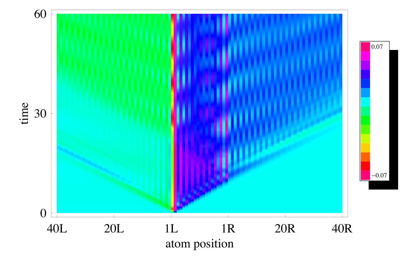
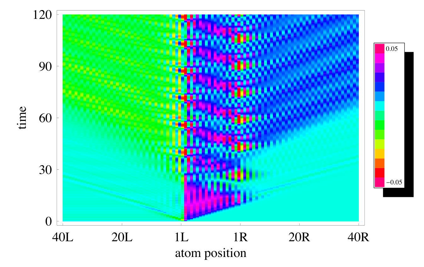
where denotes a site of the S-N-S system and the matrix element is taken over the Nambu space. We stress that our approach allows us to determine not only in the normal region, but also inside the superconducting leads[34]. This is a clear advantage with respect to the WBL approximation, in which only the dynamics of the normal region can be described. In Fig.12 we show the density variation as a function of the atomic position along the 1D S-N-S system and time. In this case a long junction with is considered. It is clearly seen at the perturbation induced by the switch-on of the bias ( and ) propagates both inside the lead (leftward) and the normal region (rightward) with velocities and respectively. At long time the density displays stationary oscillations due to the stabilization of the ac Josephson regime. In particular on the left lead the average value of is lower with respect to the one in the right lead, since . In Fig.13 we plot the transient behavior of the charge density for a junction in which the (equilibrium) condition for perfect Andreev reflection given in Eq.(33) has been imposed. Remarkably we see that no appreciable density variation inside the lead occurs before a dwelling time given by
| (48) |
where and where is the time needed to cross the normal chain between two consecutive reflections. Indeed for an electron inside the N region undergoes (almost) perfect Andreev reflections before being transmitted through the right interface. The pattern of these multiple reflections is clearly visible in Fig.13, in which the model parameters are chosen in order to have and .
VII Summary and conclusions
In this paper we have studied the dc and ac transport properties of a tight-binding S-N-S junction. In the dc case we identified three contributions to the dc Josephson current coming from the Andreev bound states, normal bound states and continuum states. The calculation of the latter contribution has been performed by employing an exact embedding procedure which consists in integrating out the superconducting degrees of freedom and in expressing the Nambu-Gorkov Keldysh Green’s function in terms of the embedding self-energy. For the bound-state contributions we calculated the phase derivative of the eigenenergies of all occupied discrete states. The secular problem is cast in terms of an effective energy-dependent Hamiltonian in which the on-site and pairing potentials of the normal chain are renormalized via the embedding self-energy. The bound-state eigenenergies of chains of arbitrary length are determined from a general equation which includes the full frequency dependence of the embedding self-energy. The limit of long-chains allows for further analytic manipulations and the ABS’s contribution to the total dc Josephson current is expressed in terms of energy-dependent phase-shifts.
For 1D superconducting leads we obtain an exact formula for the embedding self-energy at half-filling. Explicit numerical results have been presented for short and long chains, and different regimes have been analyzed. The Ishii’s sawtooth behavior results from a subtle cancellation of highly non-linear continuum and ABS’s contributions while the normal bound-state contribution vanishes. For chain hoppings smaller than half of the superconducting order parameter we numerically observed that the dc Josephson current is entirely carried by the ABS’s. This circumstance has been analytically investigated in the limit of long chains. The condition for the occurrence of the Ishii’s sawtooth behavior is expressed in terms of the microscopic parameters of the model. We here also point out a limitation of the WBL approximation, i.e. the independence of the current-phase relation from .
The ac Josephson regime was studied by applying a constant bias voltage across the junction and solving numerically the time-dependent Bogoliubov-deGennes equations for finite leads. We used the partition-free initial conditions for which the system is contacted and in equilibrium before an external driving force is switched on. If the leads are sufficiently long the results of the time propagation are the same as those of a truly infinite systems up to a critical time at which finite size effects appear.[28] Such critical time is, however, large enough to allow for studying transient responses as well as the ac Josephson regime setting in after all transient effects have been washed out. The transient time-scale is dictated by the dwelling time during which an electron undergoes several Andreev reflections before being transmitted. By extracting the dc component of the ac Josephson current we have been able to reproduce a well-defined subgap structure in the current-voltage characteristics of a S-S junction. As expected the characteristics displays kinks at biases . The time-dependent approach also permits to perform a spectral decomposition of the ac current. By Fourier transforming the curve in a proper time window we computed both the dissipative and non-dissipative components. Such procedure can be easily generalized to arbitrary time-dependent fields like, e.g., ac or pulsed biases, at the same computational cost and provides an alternative approach to Floquet-based schemes[11, 21]. We also wish to emphasize that within the present approach a full microscopic description of the superconductors is provided, and hence we are able describe the electron dynamics not only inside the normal region, but also inside the leads[34]. This allows us to gain further information with respect to the WBL approximation. In conclusion we would like to point out the proposed time-dependent approach is not limited to 1D electrodes and can be readily generalized to investigate more realistic superconductor-normal metal interfaces. In particular it would be interesting to study the case in which the normal region is two-dimensional, since it has been experimentally observed[35, 36] and theoretically predicted[37] that in such systems the ac Josephson current displays a dominant Fourier component at twice the fundamental Josephson frequency.
Acknowledgements.
E.P. is financially supported by Consorzio Nazionale Interuniversitario per le Scienze Fisiche della Materia.Appendix A Derivation of the embedding self-energy
For 1D leads the coupling is given in Eq.(14) and therefore the retarded embedding self-energy for lead in Eq.(11) reads
| (49) |
The retarded Green’s function of the uncontacted lead at half-filling is given in terms of the -dependent Bogoliubov-deGennes Hamiltonian
| (50) |
as
| (51) |
Introducing the eigenvectors
| (52) |
of with eigenvalues and taking the limit Eq.(49) becomes
| (53) |
The integral can be computed analytically to yield
| (54) |
where
| (55) |
with is a complex frequency.
The other relevant components of the Nambu self-energy are easily obtained starting from the retarded one:
| (56) |
where is the Fermi distribution function.
Appendix B Calculation of the bound states
In this Appendix we solve the eigenvalue problem in Eq.(23). We use the following ansatz[17] for the eigenstate amplitudes on the -th site of the normal region
| (57) |
where . Due to the symmetry of the problem the wavefunction must be chosen so as to fulfill the condition
| (58) |
which is equivalent to . The above condition provides an equation for the allowed wavevectors , similarly to the case of normal open chains. In the following we specialize to even . The case of odd is similar and does not introduce extra complications. We first observe that due to the choice the effective Hamiltonian in Eq.(24) is invariant under the transformation : and . It is straightforward to realize that and hence the wavefunctions obey the symmetry constraint where is a parity index. By applying the Schrodinger equation to sites 1,2 for spin and to sites for spin and exploiting the above symmetry constraint we obtain the following linear systems for the coefficients
| (59) |
where we have chosen . Indeed the proper normalization factor of the Andreev bound state wavefunction is inessential to the calculation of the bound state energy. The solution of the above system provides the -dependent coefficients
where
| (60) |
Inserting the above solution in Eq.(58) and taking into account the normalization condition one finds the following equation for the allowed values of
| (61) | |||||
Isolating the last term and squaring, the dependence on disappears and we end up with an equation valid for both parities
| (62) | |||||
which coincides with Eq.(25). The bound states eigenenergies are obtained by solving Eq.(62) numerically and retaining only the values of such that (Andreev bound states) and (normal bound states). We notice that the wavevectors for the ABS’s are real valued while for normal bound states are in general complex. Indeed for the energy lies below/above the continuum only for complex .
References
- [1] For a recent review, see e.g., G. Wendin and V.S. Shumeiko, Low Temp. Phys. 33, 724 (2007).
- [2] J.M. Martins, S. Nam, J Aumentado, and C. Urbina, Phys. Rev. Lett 89, 117901 (2002).
- [3] K.K. Likharev, Superconductor Devices for Ultrafast Computing, in Applications of Superconductivity, ed. H. Weinstock, Kluwer (1999).
- [4] V. Bouchiat, D. Vion, P. Joyez, D. Esteve, and M.H. Devoret, Phys. Scr. T76, 165 (1998).
- [5] Y. Nakamura, Yu.A. Pashkin, and J.S. Tsai, Nature (London) 398, 786 (1999).
- [6] J. Delahaye, J. Hassel, R. Lindell, M. Sillanpää, M. Paalanen, H. Seppä, and P. Hakonen, Science 299, 1045 (2003).
- [7] C.W.J. Beenakker and H. van Houten, in: Nanostructures and Mesoscopic Systems, edited by W. P. Kirk and M. A. Reed, Academic, New York (1992).
- [8] C.J. Muller, J.M. van Ruitenbeek, L.J. de Jongh, Physica C, 191, 485 (1992).
- [9] D.C. Ralph, C.T. Black, and M. Tinkham, Phys. Rev. Lett 74, 3241 (1995).
- [10] M.C. Koops, G.V. van Duyneveldt, and R. de Bruyn Ouboter, Phys. Rev. Lett 77, 2542 (1996).
- [11] J.C. Cuevas, A. Martín-Rodero, and A. Levy Yeyati, Phys. Rev. B. 54, 7366 (1996).
- [12] A. Martín-Rodero, F.J. García Vidal, and A. Levy Yeyati, Phys. Rev. Lett. 72, 554 (1993).
- [13] A.F. Andreev, Sov. Phys. JETP 19, 1228 (1964).
- [14] C.W.J. Beenakker, Phys. Rev. Lett. 67, 3836 (1991).
- [15] A. Furusaki, Superlattices Microstruct. 25, 809 (1999).
- [16] I.O. Kulik, Sov. Phys. JETP 30, 944 (1970).
- [17] I. Affleck, J.S. Caux and A.M. Zagoskin, Phys. Rev. B. 62, 1433 (2000).
- [18] A.E. Feiguin, S.R. White, and D.J. Scalapino, Phys. Rev. B. 75, 024505 (2007).
- [19] F.S. Bergeret, A. Levy Yeyati, and A. Martín-Rodero, Phys. Rev. B 76, 174510 (2007).
- [20] A. Levy Yeyati, J.C. Cuevas, A. López-Dávalos, and A. Martín-Rodero , Phys. Rev. B. 56, R6137 (1997).
- [21] G. -f. Sun, H. Guo, and J. Wang, Phys. Rev. B. 65, 075315 (2002).
- [22] Y. Xing, Q.-f Sun, and J. Wang, Phys. Rev. B. 75, 125308 (2007).
- [23] N denotes a generic non-superconducting central region, including normal metals, insulaltors, semiconductors, quantum dots, etc.. In the present work N stands for a one-dimensional tight binding chain.
- [24] R. Kümmel, Z. Physik 218, 472 (1969).
- [25] R. Kümmel, in Physics and Applications of Mesoscopic Josephson Junctions, edited by H. Ohta and C. Ishii (The Physical Society of Japan, Tokyo, 1999), p.19.
- [26] M. Cini, Phys. Rev. B 22, 5887 (1980).
- [27] G. Stefanucci and C.O. Almbladh, Phys. Rev. B 69, 195318 (2004).
- [28] E. Perfetto, G. Stefanucci and M. Cini, Phys. Rev. B 78, 155301 (2008).
- [29] In this work we set .
- [30] U. Gunsenheimer, U. Schüssler and R. Kümmel, Phys. Rev. B. 49, 6111 (1994)
- [31] C. Ishii, Prog. Theor. Phys. 44, 1525 (1970).
- [32] A.M. Zagoskin and I. Affleck, J. Phys. A: Math. Gen. 30, 5743 (1997).
- [33] G. Stefanucci, S. Kurth, A. Rubio, and E.K.U. Gross, Phys. Rev. B 77, 075339 (2008).
- [34] P. Myöhänen, A. Stan, G. Stefanucci, and R. van Leeuwen, Phys. Rev. B 80, 115107 (2009).
- [35] H. Drexler, J. Harris, E. Yuh, K. Wong, S. Allen, E. Gwinn, H. Kroemer, and E. Hu, Surf. Sci. 361/362, 306 (1996).
- [36] K. Lehnert, N. Argaman, H.-R. Blank, K. Wong, S. Allen, E. Hu, and H. Kroemer, Phys. Rev. Lett. 82, 1265 (1999).
- [37] A. Jacobs and R. Kümmel, Phys. Rev. B 71, 184504 (2005).