On the construction of the KP line-solitons and their interactions

The $\tau$-function can be expressed as the Wronskian determinant [7, 25, 24]

where $f^{(i)}$ denotes the $i^{\mathrm{t}h}$ partial derivative with respect to $x$, and where the functions $\{f_{n}\}_{n=1}^{N}$ form a set of linearly independent solutions of the linear system

A remarkable fact is that the KP equation simply turns into a determinant identity if one substitutes (3) into (1) and uses the Wronskian form of $\tau(x,y,t)$ given by (4) (see e.g., [25, 6, 23] for details). This implies that any linearly independent set of solutions of the linear system (5) will give rise to a solution of the KP equation. Hence it is possible to generate a large class of solutions in this way. In particular, the line-soliton solutions are obtained from the choice

where $\theta_{m}(x,y,t)=k_{m}x+k_{m}^{2}y+k_{m}^{3}t+\theta_{0m}$ with distinct real parameters:  $k_{1}<k_{2}<\ldots<k_{M}$ and real constants $\{\theta_{0m}\}_{m=1}^{M}$. The coefficients $(a_{nm})=:A$ define an $N\times M$ constant matrix which is of rank $N$ due to the linear independence of the functions $\{f_{n}\}_{n=1}^{N}$. Then (4) can be expressed as

by expanding the Wronskian determinant using Binet-Cauchy formula. In above, $\theta(m_{1},\ldots,m_{N}):=\theta_{m_{1}}+\theta_{m_{2}}+\ldots+\theta_{m_{N}}$, and $A(m_{1},\dots,m_{N})$ is the maximal minor, i.e., the determinant of the $N\times N$ sub-matrix of $A$ obtained from columns $1\leq m_{1}<\dots<m_{N}\leq M$. Note that the $N$ linearly independent rows of the coefficient matrix $A$ span an $N$-dimensional subspace $W$ of ${\mathbb{R}}^{M}$ so that $A$ can be regarded as a point of the real Grassmannian Gr$(N,M)$. A different choice of basis for $W$ amounts to performing row operations:  $A\to GA,\,\,G\in$ GL$(N,{\mathbb{R}})$, which changes the $\tau$-function in (7) simply by a scale factor:  $\tau\to\det(G)\tau$ but leaves the KP solution $u=2(\ln\tau)_{xx}$ invariant. Consequently the coefficient matrix $A$ can be canonically chosen in the reduced row echelon form (RREF) which has a distinguished set of pivot columns such that the restriction of $A$ to this set corresponds to the $N\times N$ identity matrix. Given any $N\times M$ matrix $A$ of rank $N$, its unique RREF gives a standard coordinate for the corresponding point in Gr$(N,M)$. It is in this sense that the space of all solutions of KP generated by the $\tau$-function given by (7) can be identified with the real Grassmann manifold Gr$(N,M)$. In general, such solutions are not all line-solitons as they can be singular where the $\tau$-function becomes zero. The regularity of the solutions in the entire $xy$-plane and for all values of $t$ is achieved by imposing a further restriction on the coefficient matrix $A$, namely that all of its $N\times N$ maximal minors be non-negative. Such matrices are called totally non-negative matrices, they represent the totally non-negative Grassmannian Gr${}^{+}(N,M)$ which forms a closed subset in Gr$(N,M)$, and which identifies the space of all line-soliton solutions of the KP equation.

Some simple examples of $\tau$-functions corresponding to some of the solutions mentioned in Section 1 are listed below.

One-soliton solution:  In this case, one chooses a single function in (6) of the form $f_{1}=e^{\theta_{1}}+e^{\theta_{2}}$. The coefficient matrix is simply $A=(1\quad 1)$, and $\tau=f_{1}$. Then equation (3) yields the one-soliton solution given by (2) in Section 1 with $\theta_{0}=\theta_{02}-\theta_{01}$. Note that since $k_{1}<k_{2}$, $\tau\sim e^{\theta_{1}}\gg e^{\theta_{2}}$ and $u(x,y,t)\sim 0$ as $x\to-\infty$. A similar argument shows that $u$ is also exponentially small as $x\to\infty$. In this case, one finds from the exact expression in (2) that the solution is localized in the $xy$-plane along the line $\theta_{1}=\theta_{2}$ (for fixed $t$) where the two exponentials in the $\tau$-function are precisely in balance (see Figure 1(a)). It turns out that even for general line-solitons, the solution $u(x,y,t)$ is localized along certain lines in the $xy$-plane where exactly two exponential terms in the $\tau$-function of equation (7) are in balance, and they dominate over all other exponential terms. This principle of dominant balance was implemented in Refs [17, 19, 20, 21] to identify the asymptotic line solitons $[i,j]$ associated with each line-soliton solution of the KP equation.

Miles Y-shape solution:  The $\tau$-function for this solution is a sum of three exponential functions, i.e., $\tau=f_{1}=e^{\theta_{1}}+e^{\theta_{2}}+e^{\theta_{3}}$ with the coefficient matrix $A=(1\quad 1\quad 1)$. Applying the dominant balance principle mentioned above, it is possible here to determine the dominant exponentials and analyze the structure of the solution in the $xy$-plane. One finds that the solution $u(x,y,t)$ is localized along three lines corresponding to the line soliton $[1,3]$ for $y\gg 1$, and line solitons $[1,2],\,[2,3]$ for $y\ll 1$ as illustrated in Figure 1(b). For $i,\,j\in\{1,2,3\}$, each line soliton $[i,j],\,i<j$ is locally of the form of the one-soliton solution (2) with distinct parameters $k_{i},\,k_{j}$. As mentioned in Section 1, the Miles solution represents a resonant solution of three line solitons. The resonant condition among those three line-solitons is given by

where ${\bf k}_{ij}={\textstyle\frac{1}{2}}(k_{j}-k_{i},k_{j}^{2}-k_{i}^{2})$ and $\omega_{ij}={\textstyle\frac{1}{2}}(k_{j}^{3}-k_{i}^{3})$ are respectively, the wave vector and frequency of the line soliton $[i,j]$, satisfying the soliton dispersion relation given in Section 1.

O-type 2-soliton solution:  Here the $\tau$-function is a Wronskian of two linearly independent solutions of (5). These solutions are obtained from (6) by choosing $N=2,\,M=4$, and the coefficient matrix

such that $f_{1}=e^{\theta_{1}}+e^{\theta_{2}}$ and $f_{2}=e^{\theta_{3}}+e^{\theta_{4}}$. Note that $A$ is a totally non-negative matrix whose $2\times 2$ maximal minors are:  $A(1,2)=A(3,4)=0$, and $A(1,3)=A(1,4)=A(2,3)=A(2,4)=1$. From (7), the resulting $\tau$-function is given by

Figure 1(c) illustrates the regions in the $xy$-plane where each of the four exponential terms in the above $\tau$-function are dominant. The line solitons corresponding to the solution $u=2(\ln\tau)_{xx}$ are $[1,2]$ and $[3,4]$ for $|y|\to\infty$; these are localized along the directions where a pair of dominant exponential terms are in balance.

The Grammian construction of the line-soliton solutions will be described next. This form of the solution arises from the so called binary Darboux transformation of the KP equation (see e.g., [24]). In this case, the $\tau$-function can be expressed as a a determinant of an $N\times N$ matrix as follows:

where $\{f_{i}\}_{i=1}^{N}$ solve (5) and $\{g_{j}\}_{j=1}^{N}$ solve the (formal) adjoint system of (5), namely,

It is easily verified from (5) and its adjoint that $d\Omega_{ij}$ is an exact differential, hence the line integral above can be evaluated along any suitable curve $\Gamma$ in the $xy$-plane such that the integral converges. Like the Wronskian form, it can be shown that the $\tau$-function in (8) yields a solution of the KP equation via (3) for any choice of the sets of functions $\{f_{i}\}_{i=1}^{N}$ and $\{g_{j}\}_{j=1}^{N}$ [6]. For the line-soliton solutions, these are chosen as linear combinations of exponentials (cf. (6)),

where $\phi(k):=kx+k^{2}y+k^{3}t+\phi_{0}(k)$, and all the parameters $p_{1},\ldots,p_{r},\,q_{1},\ldots,q_{N}$ are distinct and real. Note that $N\neq r$, in general. Thus, $B:=(b_{mn})$ is an $N\times r$ matrix whereas $\widehat{B}:=\widehat{b}_{mn}$ is an invertible, $N\times N$ matrix. Substituting (9) into the matrix elements $\Omega_{ij}$ in (8), and evaluating the line integral along a path $\Gamma$ from $({\color[rgb]{1,0,0}\mathbf{-}}\sigma\infty,\,y)$ to $(x,y)$ parallel to the $x$-axis, yields

where $\sigma=\mathrm{sgn}(p_{m}-q_{n})=\pm 1$ and $c_{ij}$ are arbitrary constants. Choosing the constants $c_{ij}=\delta_{ij}$, where $\delta_{ij}$ is the Krönecker symbol ($\delta_{ij}=0,\,i\neq j,\,\delta_{ii}=1$), ensures that the matrix $\Omega$ is of rank $N$ so that $\tau\neq 0$. Using (10), the $\tau$-function in (8) can be expressed in the form

where $C=\widehat{B}^{T}B$ is an $N\times r$ matrix of constant coefficients and $F$ is an $r\times N$ matrix whose entries are given by

The Grammian form given by the first equality in (11) is not unique as it is possible to obtain the same $\tau$-function from a different choice of the matrices $B$ and $\widehat{B}$. In particular, $\widehat{B}$ need not be a square matrix although there is always a canonical choice of an $N\times N$ matrix $\widehat{B}$ that leads to the second equality in (11). We will not discuss the details of the gauge freedom underlying the choice of $B$ and $\widehat{B}$ in this article.

Equation (11) is the canonical Grammian form for the line-soliton solutions, special cases of which arise from several direct methods of constructing solutions including the Hirota method [6], direct linearization [4] and dressing techniques [8]. For example, the O-type $N$-soliton solution is obtained by setting $r=N$ and $C=I$, the latter being the $N\times N$ identity matrix. In this case the resulting $\tau$-function $\tau=\det(I+F)$ is positive for all $x,y,t$ if the parameters are ordered as $p_{N}<p_{N-1}<\ldots<p_{1}<q_{1}<q_{2}<\ldots<q_{N}$. Then the corresponding line-soliton solution is non-singular. More general line-soliton solutions can also be generated from the Grammian form (11) by making appropriate choices for the matrix $C$. However, in comparison with the Wronskian form, here it is less clear how to impose regularity conditions on the obtained solution. Recall that in the Wronskian construction the ordering $k_{1}<k_{2}<\ldots<k_{M}$ of the parameters and the totally non-negative coefficient matrix $A$ guarantee that the KP line-soliton solutions are regular. But no such clear prescription to obtain regular solutions is known for the Grammian case. This issue can be resolved by establishing an equivalence between the Wronskian and the Grammian forms for the KP $\tau$-function. This will be done below. More specifically, it will be shown by explicit construction that there is a one-to-one correspondence between the formulas (7) and (11).

It is convenient to first start with the Wronskian form and derive the $\tau$-function formula (11) from that. It follows from either (7) or (4) that the $\tau$-function can be written as:  $\tau=\det(AEK)$, where $E=\mathrm{diag}(e^{\theta_{1}},e^{\theta_{2}},\ldots,e^{\theta_{M}})$ is an $M\times M$ diagonal matrix and $K:=(K_{ij})=(k_{i}^{j-1})$ is an $M\times N$ Vandermonde matrix. In the following, the $N\times M$ coefficient matrix $A$ will be chosen in RREF such that it can be represented as $A=(I\,,J)P$ with $I$ and $J$ denoting respectively, the $N\times N$ and $N\times(M-N)$ sub-matrices of the pivot and non-pivot columns of $A$, and $P$ being the $M\times M$ permutation matrix which shuffles those columns to form $A$. For example, the coefficient matrix for the O-type 2-soliton $\tau$-function discussed above can be represented as

where $P_{23}$ is the $4\times 4$ matrix permuting the second and the third columns. Using the above form of $A$, the determinant for the $\tau$-function becomes

where $E_{1}$ and $E_{2}$ are respectively, $N\times N$ and $(M-N)\times(M-N)$ block diagonal matrices whose elements are permutations of the set $\{e^{\theta_{1}},e^{\theta_{2}},\ldots,e^{\theta_{M}}\}$. Similarly, $K_{1}$ and $K_{2}$ are respectively, $N\times N$ and $(M-N)\times N$ matrices obtained by permuting the rows of the Vandermonde matrix $K$ by $P$. It should be clear from above that in effect, the $M\times M$ matrix $P$ induces a permutation $\pi$ of the ordered set $\{k_{1},k_{2},\ldots,k_{M}\}$ which can be expressed as

after renaming the elements of the permuted set. Accordingly, the matrices $E_{1},E_{2},K_{1},K_{2}$ are redefined as

for $i=1,\ldots,M-N,\,\,j=1,\ldots,N$, and where $\phi(k)$ is defined below (9). Since the parameters $q_{1},\ldots,q_{N}$ are distinct, the Vandermonde matrix $K_{1}$ is invertible. Then the above determinant expression for $\tau$ can be further manipulated as

where $\tau$ and $\widehat{\tau}$ differ by an exponential factor linear in $x,y,t$, hence both generate the same KP solution via (3). To show that $\widehat{\tau}$ is indeed the Grammian form of the $\tau$-function, one employs the following matrix identity which is derived in the Appendix,

where the matrices $D_{1},D_{2}$ and the Cauchy matrix $\chi$ are defined as follows:

Substitution of (13) into the expression for $\widehat{\tau}$ above, yields

Finally, by setting $r=M-N$ and the $N\times M-N$ matrix $C=D_{1}^{-1}JD_{2}$, the Grammian form of the $\tau$-function in (11) is readily recovered from the expression of $\widehat{\tau}$ above.

It is relatively straightforward to reverse the steps described above to obtain the Wronskian data, i.e., the coefficient matrix $A$ and the ordered set of parameters $k_{1}<k_{2}<\ldots<k_{M}$ from the Grammian data, which consists of the $N\times M-N$ matrix $C$ and the unordered set of parameters $\{q_{1},\ldots q_{N},p_{1},\ldots p_{M-N}\}$. The key step is to recover the permutation $\pi$ in (12) by simply ordering the set of Grammian parameters, i.e.,

This in turn, provides the $M\times M$ permutation matrix $P$ from $\pi$, and the matrix $A$ is then constructed by the formula $A=(I\,,J)P$ with $J=D_{1}CD_{2}^{-1}$, thus establishing the Grammian-Wronskian equivalence for the $\tau$-function for the KP line-soliton solutions. Such equivalence was also derived in Ref. [25] for special $N$-soliton solutions using similar techniques.

An alternative approach to obtain the Wronskian form from the Grammian in (8) that is applicable when at least one of the functions $f_{i}$ or $g_{j}$ is an exponential, was discussed in [26]. In this case, one can for instance, choose the functions $\{f_{i}\}_{i=1}^{N}$ as $N$ linearly independent solutions of (5), and $\{g_{j}:=e^{-\theta_{j}}\}_{j=1}^{N}$ with $\theta_{j}=k_{j}x+k_{j}^{2}y+k_{j}^{3}t$ and $k_{j}>0$. Using these forms of $f_{i}$ and $g_{j}$ in (8), and choosing $\Gamma$ to be the path from $(-\infty,y)$ to $(x,y)$ parallel to the $x$-axis, the integral for the matrix element $\Omega_{ij}$ can be expressed as an infinite series in inverse powers of the parameters $k_{j}$ by repeated integration by parts, provided that $f_{i}^{(n)}g_{j}\to 0,\,\,n\geq 0$ as $x\to-\infty$. Then by taking the limit $k_{j}\to\infty,\,j=1,\ldots,N$, one can recover the Wronskian form (4) from the determinant $\det(\Omega)$.

An immediate consequence of the above equivalence result is that it is now possible to formulate the regularity condition for the KP line-solitons in a precise fashion from the Grammian form (11) of the $\tau$-function. Given the matrices $C$ and $P$, a necessary and sufficient condition that the KP solution (3) is non-singular is given by the fact that $A=(I,\,J)P$ be a totally non-negative matrix. Of course, this is the same condition on the coefficient matrix $A$ in the Wronskian form. If in addition, $A$ satisfies the following irreducibility conditions:
(i)  each column of $A$ contains at least one nonzero element,
(ii)  each row of $A$ in RREF contains at least one nonzero element other than the pivot (first non-zero entry),
then the number of line solitons as $y\to\pm\infty$ in the solution generated by the $\tau$-function in (7) is determined by the size of the matrix $A$. Namely, one has $N_{-}=M-N$ and $N_{+}=N$, where $N_{\pm}$ denote the number of line solitons as $y\to\pm\infty$ [20, 21, 23]. Further analysis of the totally non-negative matrix $A$ leads to the precise identification of the line solitons and a comprehensive classification scheme for all line-soliton solutions of the KP equation. The latter problem is related to the classification of the non-negative cells Gr${}^{+}(N,M)$ of the Grassmannian Gr$(N,M)$ in terms of certain types of permutations called derangements [21].

It is worth noting that the equivalence between the Grammian and Wronskian forms of the line-soliton $\tau$-function is not unique to the KP equation but applies also to other equations whose $\tau$-functions are represented in both forms. Examples include several $2+1$-dimensional differential-difference equations such as the 2d-Toda, 2d-Volterra and the differential-difference KP equation as well as difference-difference equations such as the fully discrete 2d-Toda and the discrete KP (Hirota-Miwa) equation. These will be discussed in future works.

For the O-type, the amplitudes of the line solitons $[1,2]$ and $[3,4]$ are

the soliton phases are expressed in terms of $\theta_{j}=k_{j}x+k_{j}^{2}y+k_{j}^{3}t+\theta_{0j},\,\,j=1,\ldots,4$, as

and the constant $C$ is given in terms of the parameters $k_{1},\ldots k_{4}$ by

such that $0<C<1$. An O-type soliton is illustrated in Figure 2.

The function $u(x,y,t)$ has an absolute maximum at $\phi_{1}$ = $\phi_{2}$ = 0, and the maximum value at this interaction point is given by (see [23])

Since $C>0$, the interaction peak $u_{\mathrm{max}}$ is always greater than the sum of the individual line soliton amplitudes. In fact, one can easily verify that

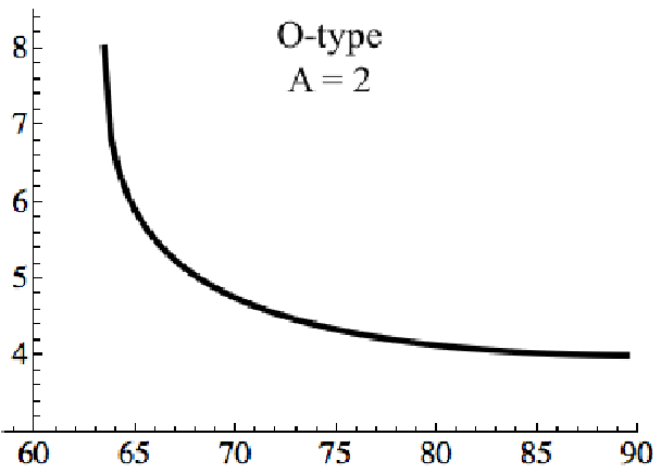
Furthermore, $u_{\mathrm{max}}$ depends non-linearly on the incidence angle between the two line solitons. In order to investigate this behavior, it is convenient to choose the parameters $k_{1},\ldots,k_{4}$ such that $k_{1}=-k_{4}$ and $k_{2}=-k_{3}=-k$ (see Figure 3(a)). Then the two line solitons are placed symmetrically about the y-axis, and are of equal amplitude, i.e., $A_{1}=A_{2}=A$. Denoting the angle between the $[3,4]$-soliton and the $y$-axis by $\psi$ as shown in Figure 3(b), it follows that $\tan\psi=(k_{3}+k_{4})=\sqrt{2A}+2k$. Since $k>0$, the angle $\psi$ is always greater than the critical angle

which depends on the amplitude of the line solitons. Setting $k_{1}=-k_{4},\,k_{2}=-k_{3}$ in the expression for $C$ above, it can be deduced from (15) that

Therefore, $u_{\mathrm{max}}$ is a decreasing function of the angle $\psi$, and as $\psi\to\psi_{c}$ (i.e., $k\to 0$), the peak interaction amplitude $u_{\mathrm{max}}\to 4A$. Note that in the limit $k=0$, the parameters $k_{2}=k_{3}$, which implies that the $\tau$-function $\tau_{\mathrm{O}}$ contains only three instead of four exponential terms. The resulting solution $u(x,y,t)$ of the KP equation is a Miles’ Y-shape solution corresponding to the confluence of three line solitons interacting resonantly [11] (see also [23]). The dependence of $u_{\mathrm{max}}$ with the angle of interaction is shown in Figure 4 for soliton amplitudes $A=1$ and $A=2$. Note that in Figure 4(a), $u_{\mathrm{m}ax}\to 4$ as $\psi$ approaches the critical angle $\psi_{c}\approx 54.7^{\circ}$, while in Figure 4(b), $u_{\mathrm{m}ax}\to 8$ as $\psi\to\psi_{c}\approx 63.4^{\circ}$.

For the P-type, the soliton amplitudes

are always unequal, and $A_{1}>A_{2}$. The soliton phases are given by

and the constant $C$ is negative since

A P-type 2-soliton solution is illustrated in Figure 5.

In contrast to the O-type, the P-type 2-soliton solution $u(x,y,t)$ corresponds to saddle at the interaction point $\phi_{1}=\phi_{2}=0$. The value of the solution at the interaction point is

Since $C<0$ for the P-type solution, $u_{\mathrm{int}}$ is always less than the sum of the amplitudes of the line solitons $[1,4]$ and $[2,3]$. A more precise bound for $u_{\mathrm{int}}$ is obtained as follows [23]: From the above expression for $C$, one can calculate

where $x={\textstyle\frac{k_{2}-k_{1}}{k_{4}-k_{1}}}$ and $y={\textstyle\frac{k_{4}-k_{3}}{k_{4}-k_{1}}}$. Since $0<x,y<1$, the following inequalities

References

- [1] B. B. Kadomtsev and V. I. Petviashvili, On the stability of solitary waves in weakly dispersive media, Sov. Phys. - Dokl. 15 (1970), pp. 539–541.
- [2] E. Infeld and G. Rowlands, Nonlinear waves, solitons and chaos, Cambridge University Press, Cambridge, 2000.
- [3] S. Novikov, S. V. Manakov, L. P. Pitaevskii and V. E. Zakharov, Theory of Solitons: The Inverse Scattering Method, Contemporary Soviet Mathematics, Consultants Bureau, New York and London, 1984.
- [4] M. J. Ablowitz and P. A. Clarkson, Solitons, nonlinear evolution equations and inverse scattering, Cambridge University Press, Cambridge, 1991.
- [5] L. A. Dickey, Soliton equations and Hamiltonian systems, Advanced Series in Mathematical Physics Vol. 12, World Scientific, Singapore, 1991.
- [6] R Hirota, The Direct Method in Soliton Theory, Cambridge University Press, Cambridge, 2004.
- [7] M. Sato, Soliton equations as dynamical systems on an infinite dimensional Grassmannian manifold, RIMS Kokyuroku (Kyoto University) 439 (1981), pp. 30–46.
- [8] V. E. Zakharov and A. B. Shabat, A scheme for integrating nonlinear equations of mathematical physics by the method of the inverse scattering problem, Func. Anal. Appl. 8 (1974), pp. 226–235.
- [9] J. Satsuma, -Soliton solution of the two-dimensional Korteweg-de Vries equation, J. Phys. Soc. Jpn. 40 (1976), pp. 286–290
- [10] N. C. Freeman and J. J. C. Nimmo, Soliton-solutions of the Korteweg-de Vries and Kadomtsev-Petviashvili equations: the Wronskian technique, Phys. Lett. A 95 (1983), pp. 1–3.
- [11] J. W. Miles, Resonantly interacting solitary waves, J. Fluid Mech. 79 (1977), pp. 171–179.
- [12] A. C. Newell and L. G. Redekopp, Breakdown of Zakharov-Shabat theory and soliton creation, Phys. Rev. Lett. 38 (1977), pp. 377–380.
- [13] N. C. Freeman, Soliton interactions in two-dimensions, Adv. Appl. Mech. 20 (1980), pp. 1–37.
- [14] K. Ohkuma and M. Wadati, The Kadomtsev-Petviashvili equation: the trace method and the soliton resonances, J. Phys. Soc. Jpn. 52 (1983), pp. 749–760.
- [15] M. Boiti, F. Pempinelli, A. K. Pogrebkov and B. Prinari, Towards an inverse scattering theory for non-decaying potentials of the heat equation, Inverse Problems 17 (2001), pp. 937–957.
- [16] E. Medina, An soliton resonance for the KP equation: interaction with change of form and velocity, Lett. Math. Phys. 62 (2002), pp. 91–99.
- [17] G. Biondini and Y. Kodama, On a family of solutions of the Kadomtsev-Petviashvili equation which also satisfy the Toda lattice hierarchy, J. Phys. A: Math. Gen. 36 (2003), pp. 10519–10536.
- [18] O. Pashaev and M. Francisco, Degenerate four virtual soliton resonance for the KP-II Theor. Math. Phys. 144 (2005), pp. 1022–1029.
- [19] Y. Kodama, Young diagrams and -soliton solutions of the KP equation, J. Phys. A: Math. Gen. 37 (2004), pp. 11169–11190.
- [20] G. Biondini and S. Chakravarty, Soliton solutions of the Kadomtsev-Petviashvili II equation, J. Math. Phys. 47 (2006), 033514i (26 pp).
- [21] S. Chakravarty and Y. Kodama, Classification of the line-solitons of KPII, J. Phys. A: Math. Theor. 41 (2008), 275209 (33 pp).
- [22] S. Chakravarty and Y. Kodama, A generating function for the -soliton solutions of the Kadomtsev-Petviashvili II equation, Contemp. Math. 471 (2008), pp. 47–67.
- [23] S. Chakravarty and Y. Kodama, Soliton solutions of the KP equation and application to shallow water waves, Stud. Appl. Math. 123 (2009), pp. 83–151.
- [24] V. B. Matveev and M. A. Salle, Darboux Transformations and Solitons Springer-Verlag, Berlin 1991.
- [25] N. C. Freeman and J. J. C. Nimmo, Soliton solutions of the Korteweg-de Vries and Kadomtsev-Petviashvili equations: the wronskian technique, Proc. R. Soc. Lond. A389 (1983), pp. 319–329.
- [26] V. M. Galkin, D. E. Pelinovsky and Yu. A. Stepanyants, The structure of the rational solutions to the Boussinesq equation, Physica D 80 (1995), pp. 246–255.
Appendix A
Here we provide an elementary derivation of the matrix identity (13) involving the Vandermonde matrices and . Recall that is an matrix with elements , and is an matrix with elements where is a set of distinct elements.
Consider monic polynomials such that each polynomial is of degree and has distinct real roots which consist of elements from the set . These polynomials can be expressed as