Free energy calculations: An efficient adaptive biasing potential method

Consider a system whose configuration is described by a variable $x\in{\mathcal{X}}$, where ${\mathcal{X}}$ is the configuration space. We denote by $V$ the potential energy function. Assume that we are given a $N$-dimensional reaction coordinate $\xi(x)$ with values in $\Omega$, which characterizes some physical event. The density of states at a value $\xi^{*}$ of the reaction coordinate is defined as

where $\beta=1/(k_{B}T)$, and $Z$ is a normalization constant, chosen such that

Eq. (1) defines the free energy $A(\xi^{*})$. Recall that, in practice, the free energy needs only be known up to an additive constant since the important quantities to describe the relative likelihoods of physical states are free-energy differences.

In general, the free energy is unknown and has to be approximated. The method we propose in this work is based on the following limit:

where

with for instance a Gaussian approximation of the Dirac delta function:

Equation (2) defines an approximate free energy $A_{\alpha}$, obtained by sampling the density of states at a finite $\alpha$, i.e., by sampling a mollified density of states. Notice that the approximation resulting from finite $\alpha$ can in fact be rewritten as a convolution of the actual density of states $e^{-\beta A}$ with $\delta_{\alpha}$. Indeed,

This remark is the basis for an extraction of the actual free energy $A$ from $A_{\alpha}$ through a deconvolution procedure (see Section IV.1). While we make this presentation with a scalar $\alpha$, this could easily be generalized to the case where $\alpha$ takes different values in different dimensions of the reaction coordinate.

Equation (3) is also helpful in assessing the errors introduced in umbrella sampling (US) and thermodynamic integration (TI) simulations employing harmonic constraint potentials. The corresponding error is analogous to the convolution errors discussed in this paper. Note that the parameter $\alpha$ can be converted to a force constant for a harmonic potential via $k=2k_{B}T/\alpha^{2}$, where $k$ is the force constant. Errors resulting from finite $k$ in TI and US computations can be identified as resulting from a convolution between the true density of states and a known Gaussian function. Typically, the harmonic constraints are tight enough for $A_{\alpha}$ to be a good approximation of $A$ but any persisting bias can, at least in principle, be removed by deconvolution as shown below.

In this work, we use $A_{\alpha}$ to define an adaptive bias. The first interest of this approach is that the gradient of $A_{\alpha}$ is much easier to compute than the gradient of $A$. Indeed, the laster reads (see References [10, 11, 12])

where $\langle\cdot\rangle_{\xi^{*}}$ denotes a canonical average for a fixed value of the reaction coordinate, and $G$ is the Gram matrix. The latter matrix is defined as $G=JJ^{t}$ with $J_{ij}=\partial\xi_{i}/\partial x_{j}$ ($x_{i}$ are the Cartesian coordinates on which the reaction coordinates are defined). The computation of the free energy gradient therefore requires the computation of second derivatives of the reaction coordinate, which is cumbersome in many cases. The gradient of the mollified free energy has a much simpler expression:

where $j$ is a reaction coordinate index and

In particular, no derivative of the reaction coordinates are required.

Another interest of the mollified free energy lies in the nonlocality of $\delta_{\alpha}$, which allows a single observation of $\xi$ to contribute to $A_{\alpha}$ for a range of values $\xi^{*}$, leading to a faster convergence. The question is then whether there is a range of $\alpha$ for which: (i) $\alpha$ is sufficiently large so that $A_{\alpha}$ could be estimated with fewer samples than what would be required to compute $A$ and (ii) $\alpha$ is sufficiently small, so that $A_{\alpha}$ is close enough to $A$ to efficiently bias the dynamics. We show in Section IV.3 that a large range of $\alpha$ satisfies these two conditions on a paradigmatic test case.

Self-healing umbrella sampling[5] (SHUS) can be seen as a special case of the method presented here. SHUS can be written in terms of Eq. (12) using the following time-dependent constant:

With this choice we have, $V_{b}=-A_{\alpha}$ and $\int_{\Omega}e^{\beta V_{b}(\xi,t)}\,d\xi=1$. This choice for $c(n)$ was suboptimal since the analysis of section II.3.3 shows that the value of $c$ should be as large as possible. Notice also that when the reaction coordinate space is discretized into a finite number of bins, the normalization condition (7) should be restated as a sum over bin indexes and the maximal value of $\exp[-\beta A_{\alpha}(\xi,n)]$ is therefore less than one. This corresponds to a negative value of $c(n)$. We checked for the testcase considered in Section IV that our method outperforms SHUS for precisely this reason.

We compare numerically our approach to two ABF formulations in Section IV.1. ABF is a good reference for comparison because there are no model parameters to choose. Errors arise only through time and reaction coordinate discretization. Two exact formulations of the free energy gradient are (4) above, and

where $M_{\xi}^{-1}=JMJ^{t}$ with $M$ the mass matrix and $J$ defined in (4) (see reference [8] for this second expression). We point out that in practice $F(\xi)$ is approximated by a trajectory average $F(\xi,t)$ which is then used to bias the dynamics. For further details on the expressions (4) and (15) or their numerical implementation, we refer the reader to the cited works.

With ABF, one must address constructing the free energy from an estimation of its gradient, the calculated field $F$. While there are specific solutions to this problem[8, 14, 15] we employ a standard variational formulation. We recast this question as an optimization problem where the objective function

is to be minimized. The corresponding Euler-Lagrange equation is

which is just Poisson’s equation, to be supplemented with appropriate boundary conditions (depending on the domain $\Omega$). The solution $u(\xi)$ is the best representation of the free energy given the vector field $F(\xi)$. This is solved via finite difference in the present work, but finite elements (or any Galerkin method) could be used as well.

Because we have developed a method within the adaptive bias potential paradigm, we also make a comparison to well-tempered metadynamics[16]. In this formulation of metadynamics the bias potential in one dimension is given by

where the functions $G(X,H,W)$ are Gaussians of width $W$ and height $H$, centered on $X$. We write $V_{b}^{\rm meta}$ to indicate that this is the bias potential generated by metadynamics. The Gaussian height in well-tempered metadynamics is both dependent on time and position along the reaction coordinate $h(\xi,t)=\omega\exp[-V_{b}^{\rm meta}(\xi,t)/k_{B}\Delta T]\tau_{G}$. For details of this version of metadynamics we refer the reader to reference [16]. We compare to this particular formulation because it requires less interaction with the user and a choice of parameter values is given in the cited reference.

Alanine dipeptide is a familiar system for benchmarking sampling methods[17, 14, 18, 16, 8, 19]. Here, we employ AMBER with a half femtosecond timestep, no constraints, solvent effects are modeled with the generalized Born model and we use the ff94 parameterization. The temperature was maintained at $T=300$K with Langevin dynamics where the collision frequency is $1$ ps^-1. We select the common backbone dihedral angles $(\xi_{1},\xi_{2})=(\Phi,\Psi)$ as reaction coordinates.

When discretizing the reaction coordinate, it is common to use a small bin size to be sure that the free energy is correctly captured. Here, we use $300$ bins of width $1.2$ degrees. We will also consider a bin width of $3.6$ degrees for Eq. (15) to examine the influence of bin size on ABF. In practice, for Eqs. (13) and (14), the current configuration along a trajectory may contribute only to an $m$ by $m$ grid centered around $(\xi_{1}(x_{t}),\xi_{2}(x_{t}))$, which amounts to truncating the range of the Gaussian function $\delta_{\alpha}$. The number of bins $m$ were chosen so that $\delta^{\prime}_{\alpha}(\xi-\xi^{*})$ is negligible for $\xi^{*}$ outside this box. For example, when $\alpha=5^{\circ}$ we use $m=20$. In practice we neglect the normalization $Z_{n}$ as well as the normalization of $\delta_{\alpha}$. We give a schematic algorithm in appendix A.

In simulations with equations (13), (4) and (15), we use a “ramp function” $R(N_{l,k})=\min[1,N_{l,k}/N_{0}]$ to scale the biasing force (see for instance reference [8]), where $N_{l,k}$ is the population in bin $(l,k)$ and the parameter $N_{0}=10$ was optimized for equations (4) and (15). The ramp function scales the biasing force so that the initially noisy observations of the force do not induce non equilibrium effects. The biasing force for the method presented here is given by Eq. (14). The biasing force for the ABF methods are given in equations (4) and (15). The biasing forces (and biasing potential) are updated at each timestep.

To study sampling efficiency we use the average difference

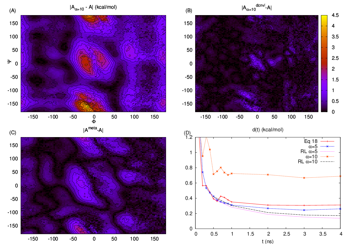
between the estimated free energy and a reference to be defined below. $n$ is the number of bins in each coordinate, $k$ and $l$ are bin indices. For Eq. (4) and (15) $\hat{A}$ is the solution of Eq. (17). In out method, $\hat{A}$ is either the left-hand side of Eq. (13), $A_{\alpha}$, or its deconvoluted version $A_{\alpha}^{\rm dcnvl}$. Finally for Eq. (18), $\hat{A}=-(T+\Delta T)V_{b}^{\rm meta}/\Delta T$. The reported results for $d(t)$ are found by using only a single trajectory with each method. We do not report the results obtained with SHUS since the convergence was found to happen much slower than for cases where $c>0$.

We use the Richardson-Lucy algorithm[20, 21] to deconvolute $A_{\alpha}$ because of its simplicity but another method of deconvolution could be used, in particular if $\delta_{\alpha}$ is not defined as a Gaussian. This algorithm is denoted by “RL” throughout. The RL algorithm uses the following iterative procedure:

where $f_{0}(\xi)=\exp[-\beta A_{\alpha}(\xi)]$, which is given by equation (13). To begin the algorithm, $\delta_{\alpha}$ and $f_{i}$ must be normalized. The fixed-point iteration (20) suggests that $f_{n}(\xi)\rightarrow\exp[-\beta A(\xi)]$ as $n\to+\infty$. We use 10 iterations in the reported results.

The reference free energy was computed by reweighting a long biased trajectory (120 ns) as

where $V_{b}(\xi,\tau)$ was constructed from 4 ns of simulation with the mollified DOS method. The bias was not updated during construction of the reference free energy. This produces a result free from errors associated with the choice of $\alpha$. The reference profile $A_{\text{ref}}$ is shown in figure 1(A) and in figure 1(B) we show $A_{\alpha}(\xi,t)$ at 1 ns of sampling with $\alpha=5^{\circ}$. The average difference $d(t)$ is shown in figure 2 for $A_{\alpha}$ with different values of $\alpha$. To show how the zero of energy of the bias potential controls the speed of convergence, in figure 2 we plot Eq. (13) with $c=0$ in (12) and we set $c=15k_{B}T$ for the remaining simulations. In figure 3 we show $d(t)$ for Eqs. (4) and (15) (ABF methods). Results for Eq. (18) (well-tempered metadynamics) are shown in figure 4(D).

For small $\alpha$ the nonlocality of the formulation disappears and in figure 2 we see slow convergence for $\alpha=0.8^{\circ}$. For intermediate values of $\alpha$, nonlocality allows the bias potential to equilibrate much faster. For $\alpha=2^{\circ}$ and $\alpha=5^{\circ}$, $A_{\alpha}$ is a good approximation of $A$, $d(t)$ falls well under $1$ kcal/mol and we observe high efficiency. With the value $\alpha=10^{\circ}$, $d(t)$ plateaus at roughly $1$ kcal/mol; $\alpha$ is now too large for $A_{\alpha}$ to be a good approximation of $A$. After applying the RL deconvolution to $A_{\alpha=10^{\circ}}$, $d(t)$ drops to match the accuracy obtained with $\alpha=2^{\circ}$ or $\alpha=5^{\circ}$. The correspondence between $A_{\alpha}$ and $A$ has deteriorated but not enough to decelerate the sampling: $A_{\alpha=10^{\circ}}$ is still a good biasing potential and $A$ can be recovered with deconvolution even at very short times.

For large $\alpha$ Eq. (14) approaches zero, leaving only a small biasing force to accelerate the dynamics. To assess whether $\alpha=20^{\circ}$ is so large as to slow down the sampling, we apply the RL deconvolution. The results in figure 2 demonstrate that $A$ can be recovered to high accuracy for $\alpha=20^{\circ}$ at long times but that sampling efficiency is affected.

In figure 3 we show $d(t)$ for Eqs. (4) and (15) with a bin size of $1.2^{\circ}$ and also for Eq. (15) with a bin width of $3.6^{\circ}$. If we compare the time to reach $d(t)=1$ kcal/mol, simulation with Eq. (13) is roughly three to ten times faster than Eqs. (4) and (15) for $2\leq\alpha\leq 20$ at the bins size of $1.2^{\circ}$. For the larger bin size $3.6^{\circ}$, ABF sampling speed becomes competitive with the mollified density of states approach but it is impossible to remove the error. The $3.6^{\circ}$ bin width coincides with the Gaussian half-width of $\delta_{\alpha}$ when $\alpha=2^{\circ}$. A larger bin size can enhance sampling speed for ABF but at a cost in accuracy. Note that $\alpha=20^{\circ}$ corresponds to a $\delta_{\alpha}$ with a half width that spans $33.3^{\circ}$ in one dimension. This is a very large effective bin width for the accuracy of the results; A similar bin size with Eqs. (4) or (15) would produce large, irreparable errors.

In figure 4 we show results for the metadynamics simulations. We use the values $\Delta T=1800$ K, $\omega=0.24$ cal mol^-1 fs^-1 and $\tau_{G}=120$ fs, as suggested in reference [16]. We could not improve the results by choosing different parameters. In panels (A) and (B) of figure 4 we show the absolute difference between the computed $A_{\alpha=10}$ and the reference $A$ with and without deconvolution, respectively. Clearly, the bulk of error is due to the missrepresentation of the very negatively curved regions of the free energy and the ability to deconvolute $A_{\alpha}$ drastically reduces this error. In panel (C) we show the absolute difference between the free energy computed via equation (18) and the reference. We see again that the error is concentrated in the regions of large negative curvature but there is not simple and obvious way to reduce these errors with some post-process. Panel (D) confirms that the metadynamics promotes extremely rapid sampling but that the long time accuracy, especially in strongly curved regions, is limited.

The results summarized in figures 2, 3 and 4 imply that a wide range of values $2\leq\alpha\leq 20$ lead to good efficiency. The ability to use the simple deconvolution algorithm is a clear advantage of the method.

We now discuss how to a priori choose $\alpha$ based on some rough error estimates. Taking $\xi$ as a scalar, we may expand $e^{-\beta A(\xi^{*})}$ as a Taylor series. Eq. (3) yields

where we keep terms up to the second moment of $\delta_{\alpha}$. Assuming that $A(\xi)$ is harmonic near the minimum $\xi=q$, the curvature can be estimated as $A^{\prime\prime}(q)=k_{B}T/\sigma^{2}$ where $\sigma^{2}$ is the variance of the reaction coordinate at temperature $T$. From Eq. (21),

While the higher order terms and the regions where $A^{\prime}\neq 0$ are certainly important to the total error, this motivates defining $\alpha$ as a function of $\sigma$ if little is known about the free energy — we can always calculate $\sigma$ in the initial state.

We calculate the variance of the reaction coordinates to be about $\sigma^{2}=340$ degrees squared for both $\Phi$ and $\Psi$. In terms of the values of $\alpha$ discussed above, this implies $\sigma/9\leq\alpha\leq\sigma/2$ as a good range for fixing $\alpha$ from calculation of $\sigma$. Of course, different $\alpha$’s may also be used for different coordinates.

References

- [1] P. Hänggi, P. Talkner, and M. Borkovec, Rev. Mod. Phys. 62, 251 (1990).
- [2] F. Wang and D. P. Landau, Phys. Rev. E 64, 056101:1 (2001a).
- [3] E. Darve and A. Pohorille, J. Chem. Phys. 115, 9169 (2001).
- [4] A. Laio and M. Parrinello, Proc. Natl. Acca. Sci. 99, 12562 (2002).
- [5] S.Marsili, A. Barducci, R. Chelli, P. Procacci, and V. Schettino, J. Phys. Chem. B 110, 14011 (2006).
- [6] L. Maragliano and E. Vanden-Eijnden, Chem. Phys. Lett. 426, 168 (2006).
- [7] T. Lelièvre, M. Rousset, and G. Stoltz, J. Chem. Phys. 126, 134111:1 (2007).
- [8] E. Darve, D. Rodriguez-Gomez, and A. Pohorille, J. Chem. Phys. 128, 144120:1 (2008).
- [9] F. Wang and D. P. Landau, Phys. Rev. Lett. 86, 2050 (2001b).
- [10] W. den Otter and W. Briels, J. Chem. Phys. 109, 4139 (1998).
- [11] M. Sprik and G. Ciccotti, J. Chem. Phys. 109, 7737 (1998).
- [12] G. Ciccotti, T. Lelièvre, and E. Vanden-Eijnden, Commun. Pure Appl. Math. 61, 371 (2008).
- [13] T. Lelièvre, M. Rousset, and G. Stoltz, Nonlinearity 21, 1155 (2008).
- [14] L. Maragliano and E. Vanden-Eijnden, J. Chem. Phys. 128, 184110:1 (2008).
- [15] J. Kästner, J. Chem. Phys. 131, 034109:1 (2009).
- [16] A. Barducci, G. Bussi, and M. Parrinello, Phys. Rev. Lett. 100, 020603:1 (2008).
- [17] C. Bartels and M. Karplus, J. Comp. Chem. 18, 1450 (1997).
- [18] B. Strodel and D. Wales, Chem. Phys. Letts. 466, 105 (2008).
- [19] X. Li, R. A. Latour, and S. J. Stuart, J. Chem. Phys. 130, 174106:1 (2009).
- [20] W. Richardson, J. Opt. Soc. Am. 62, 55 (1972).
- [21] L. Lucy, AJ 79, 745 (1974).