BI-TP 2009/26
November 2009
Longitudinal and transverse spectral functions
in the three-dimensional model
J. Engels and O. Vogt
Fakultät für Physik, Universität Bielefeld, D-33615 Bielefeld, Germany
Abstract
We have performed a high statistics simulation of the model on a three-dimensional lattice of linear extension for small external fields . Using the maximum entropy method we analyze the longitudinal and transverse plane spin correlation functions for and . In the transverse case we find for all and a single sharp peak in the spectral function, whose position defines the transverse mass , the correlator is that of a free particle with mass . In the longitudinal case we find in the very high temperature region also a single sharp peak in the spectrum. On approaching the critical point from above the peak broadens somewhat and at its position is at for all our values. Below we find still a significant peak at and at higher values a continuum of states with several smaller peaks with decreasing heights. This finding is in accord with a relation of Patashinskii and Pokrovskii between the longitudinal and the transverse correlation functions. We test this relation and its range of applicability in the following. As a by-product we calculate critical exponents and amplitudes and confirm our former results.
PACS : 64.10.+h; 75.10.Hk; 05.50+q
Keywords: model; Correlation functions; Maximum Entropy Method;
Spectral function
Corresponding author: Jürgen Engels
Fakultät für Physik, Universität Bielefeld, D-33615 Bielefeld, Germany
Tel.: +49 521 1065317, Fax: +49 521 1062961
E-mail addresses: engels@physik.uni-bielefeld.de, o-vogt@t-online.de
1 Introduction
spin models with possess two types of two-point correlation functions, one for the transverse and and one for the longitudinal spin component, defined relative to the direction of the external field . Correspondingly, there exist also two distinct susceptibilities and correlation lengths. The difference and interplay between the two sets of observables is of interest not only for the critical behaviour near to , the critical temperature, but as well for the study of the singularities induced by the existence of the massless Goldstone modes in these spin models for dimension and all [1, 2].
In a previous paper [3] we studied the correlation lengths which govern the exponential decay of the two correlation functions in the three-dimensional -model on lattices of linear extensions . We were able to confirm the predicted singular Goldstone behaviour [4, 5] of the transverse correlation length near the coexistence line, and to determine the scaling function of . For the longitudinal correlation length the situation was different. In the high temperature region the scaling function could be calculated, in the low temperature phase, , we were however unable to reliably estimate , the data were not even scaling. This was ascribed to a spectrum of higher states which contribute to the longitudinal correlators below . In this paper we want to calculate the spectral functions of the two correlators and to actually find these states above the ground states . Here, not only the spectrum of the longitudinal correlator is of interest, but as well the transverse spectrum. Spin-wave theory assumes, that long-wavelength transverse fluctuations dominate for small fields in thermal equilibrium below and that these fluctuations are describable by the Gaussian model or free field functional. This assumption can be tested readily by comparing the transverse correlator to the known Gaussian form. Of course, no higher state should then appear in the spectrum.
The resulting dependence on of the lowest states and at fixed can be utilized to test critcal behaviour and the effects of massless Goldstone modes. At the critical point we had already found in Ref. [3] that , like for [6]. The equation between the two masses or correlation lengths follows from a relation between the transverse and longitudinal correlation functions [5, 4] which should be valid for small in the whole low temperature phase. We shall discuss and test this relation explicitly for its range of applicability. In order to achieve these goals, we simulate the -invariant nonlinear -model with high statistics on a lattice with linear extension . We have chosen this specific model for several reasons: first because we want to clarify the open points raised in Ref. [3], second because in contrast to the corresponding -model corrections to scaling are negligible here, and third because the model is of relevance for quantum chromodynamics (QCD) with two degenerate light-quark flavours at finite temperature, since its phase transition is supposed to belong to the same universality class as the chiral transition of QCD [7, 8, 9].
The -model which we study here is defined by the Hamiltonian
| (1) |
where and are nearest-neighbour sites on a three-dimensional hypercubic lattice with periodic boundary conditions, and is a -component spin vector at site with length 1. It is convenient to give the following formulas still for general , though we use in our simulations . The magnetization vector is the expectation value of the lattice average of the local spins
| (2) |
Here, and is the number of lattice points per direction, the lattice spacing is fixed to 1. Due to the invariance of , the -independent part of , under -rotations of , the magnetization vector aligns with
| (3) |
It is therefore appropriate also to decompose the spin vectors into longitudinal (parallel to the magnetic field ) and transverse components
| (4) |
The order parameter of the system, the magnetization , is then the expectation value of the lattice average of the longitudinal spin components
| (5) |
Owing to the components of and one is led to a whole matrix of susceptibilities
| (6) |
with . The matrix can be expressed with only two quantities
| (7) |
the longitudinal and the transverse susceptibility. The total susceptibility is
| (8) |
From the last equation and
| (9) |
one finds, as expected, that the transverse susceptibility corresponds to the fluctuation per component of the lattice average of the transverse spin components
| (10) |
The two susceptibilities can as well be obtained from the equations
| (11) |
The remainder of the paper is organized as follows. We start with a detailed discussion of the correlation functions and their properties, the formula connecting the two types of correlators and their spectral representations. In Section 3 we address the critical behaviour of the observables. In the following Section 4 we describe some details of our simulations and the used maximum entropy method (MEM). Then we analyze our data in the different -regions: below , at and in the high temperature region; first separately for the transverse and longitudinal correlation functions, subsequently we investigate their interplay. We close with a summary and the conclusions.
2 The correlation functions
2.1 2-Point correlators
As for the susceptibilities, there exists a matrix of 2-point connected correlation functions
| (12) |
Furthermore, because of translation invariance we have
| (13) |
The correlation functions are related to the susceptibilities by
| (14) |
The matrix must have the same form as the matrix
| (15) |
leading to
| (16) | |||||
| (17) |
As mentioned already, the large distance behaviour of the correlation functions is determined by the respective exponential correlation lenghts
| (18) |
This is true for all temperatures (the coupling acts here as inverse temperature, that is ) and external fields , except on the coexistence line and at the critical point, where the correlation lengths diverge.
2.2 2-Plane correlators
Instead of the 2-point correlation functions we shall actually measure 2-plane correlation functions. They are defined as the connected correlation functions of spin averages over planes. For example, the spin average over the -plane at position is
| (19) |
The general 2-plane connected correlation functions are then
| (20) |
Also the expectation values of the longitudinal and transverse components of are independent of and equal to those of the corresponding lattice averages
| (21) |
The respective longitudinal and transverse plane-correlation functions are
| (22) | |||||
| (23) |
Here, is the distance between the two planes. Instead of choosing the -direction as normal to the plane one can as well take the - or -directions. Accordingly, we enhance the accuracy of the correlation function data by averaging over all three directions and all possible translations. The correlators are symmetric and periodic functions of the distance between the planes, the factor on the right-hand sides of (22) and (23) ensures the relation
| (24) |
Like the point-correlation functions in Eq. (18) the plane correlators decay exponentially.
2.3 The Gaussian model
We noted already in the introduction, that the Gaussian model is assumed to describe the long-wavelength transverse fluctuations. Therefore, we shortly discuss, following Ref. [10], the aspects of the model which are relevant for our work, first in dimensions, finite volume and the continuum limit. Here, is a single component, real scalar field with the Hamiltonian
| (25) |
where is the so-called stiffness and is proportional to the square of the mass of the field. Let us introduce the Fourier transform of the field
| (26) | |||||
| (27) |
For periodic boundary conditions, the components of are restricted to with and because is real we have . In terms of the Hamiltonian is
| (28) |
that is the decouple,
| (29) |
That leads to the results
| (30) |
The latter expectation value is thus directly the 2-point connected correlator of . It is easy to evaluate the Gaussian correlator for , the case of the 2-plane correlation function
| (31) |
Here, and the mass is . Using the well-known relation
| (32) |
for , we obtain
| (33) |
In addition, we can identify with the inverse of the susceptibility
| (34) |
In the infinite volume limit, , the Gaussian correlator is
| (35) |
The integral is known for general [10, 11]
| (36) |
where is a modified Bessel function. We are interested here in the two cases
| (37) | |||||
| (38) |
The last equation can also be obtained from Eq. (33) for .
2.4 The relation between the transverse and longitudinal
correlation functions
The connection between the two correlation functions was first established in a paper by Patashinskii and Pokrovskii [5]. The main arguments leading to this relation are the following. The transverse susceptibility , Eq. (11), obviously becomes infinite for all and , due to the non-zero spontaneous magnetization in the low temperature phase. The instability comes about because of infinitesimal long-wavelength transverse fluctuations which change the direction of but not its length . For a fluctuation
| (39) |
the length change is
| (40) |
To lowest order in length conserving fluctuations
| (41) |
entail longitudinal fluctuations of size
| (42) |
Patashinskii and Prokrovskii extend this ”principle of conservation of the modulus” also to local fluctuations, that is to non-uniform spin-waves with long wavelengths
| (43) |
The longitudinal correlation function can then be expressed as
| (44) | |||||
| (45) |
In the last expectation value we have explicitly noted that the connected value has to be taken. As already mentioned, the transverse fluctuations are assumed to have the Gaussian form of Eq. (25)
| (46) |
The stiffness depends on the temperature and is to lowest order independent of . It measures the resistance of the system against non-uniform rotations of . In the disordered phase, where the correlation length is finite, distant points can have different orientations and should be essentially 1. From Eq. (46) it is clear that the components of do not interact, since
| (47) |
and the components decouple. We may therefore use Wick’s theorem to reduce the expectation value in Eq. (45)
| (48) |
so that
| (49) |
where we have used Eq. (15). That finally leads to
| (50) |
Let us briefly discuss the consequences of Eq. (50), the PP-relation, in the infinite volume limit. The transverse correlation function is then given by Eq. (37) with the mass and
| (51) |
whereas the longitudinal correlation function is
| (52) |
The Fourier transform of is
| (53) |
where . It is instructive to compute the corresponding longitudinal susceptibility
| (54) |
or
| (55) |
The last equation implies the divergence of for and . That is exactly the singular Goldstone behaviour predicted in Refs. [12] and [1, 2] from field theory. Furthermore, we find from Eq. (51) that near the coexistence line
| (56) |
and from Eq. (50), if is decaying exponentially
| (57) |
In order to test all these relations with our data we need the lattice versions of the one-pole correlation functions, Eqs. (37) and (38), and the corresponding predictions from the PP-relation (50). On a lattice with periodic boundary conditions the Fourier transforms are
| (58) |
where with and with for even . Evidently, the 2-plane correlation function is proportional to the sum of exponentials
| (59) |
The normalization factor is determined by Eq. (24), so that
| (60) |
For small the prefactor
| (61) |
coincides with that of Eq. (33). The Fourier transform of is
| (62) |
As in Ref. [13] we extend the form (62) to the three-dimensional Fourier transform
| (63) |
from which is obtained, using Eq. (58). Once we have determined from MEM or a direct fit of the transverse 2-plane correlator data to Eq. (60), we can compare the longitudinal data to the following predictions from the PP-relation. Let us first compute the longitudinal susceptibility
| (64) |
From
| (65) |
where the prime on the sum indicates that there is no contribution from , we find
| (66) | |||||
| (67) |
In the last equation we have used Eq. (61) and . Similarly, we can find the longitudinal 2-plane correlator from
| (68) |
Here, we have
| (69) |
or
| (70) | |||||
2.5 The spectral functions
We define the spectral function of the 2-plane correlation function by the integral equation
| (71) |
where the integral kernel is
| (72) |
This choice of the kernel is motivated on one hand by the lattice form of the 2-plane correlators as obtained in the transfer matrix (TM) formalism [13] and second from the appearance of the same factor in the continuum, Eq. (33), and lattice forms, Eq. (60), of the one-pole correlation function. Moreover, this kernel corresponds to the one known from finite temperature QCD [14, 15], where is replaced by . Yet, we are free to redefine the kernel and the spectral function by a convenient factor and its inverse such that remains invariant. In a paper by Aarts et al. [16] this freedom has been used to remove numerical instabilities in Bryan’s MEM-algorithm [17] at small which are due to the singularity of the kernel at by changing the kernel with the factor (in our notation)
| (73) |
Here, as for the original kernel , the limits and of do not commute, because of the additional factor in . Unfortunately, not only the small but also the large -dependence of the kernel is changed by the choice (73). We arrive at a more adequate redefinition by first noting that for finite in the continuum
| (74) |
and on the lattice
| (75) |
The choice
| (76) |
normalizes then in to 1, independent of , and leads to the sum rule
| (77) |
This approach has several advantages: it cures the numerical problems appearing in Bryan’s algorithm, the limits of for and are finite and commute, and the large -behaviour remains unchanged on the lattice. From the measured the sum rule gives us already some information on the size of before we start to calculate it. We note here, that the bosonic kernel had been redefined earlier by Jarrel and Gubernatis [18] with a factor to ensure positive definite spectra.
In applying the maximum entropy method a default model for the spectral function is required which represents prior knowledge about and accordingly . Quite obviously the transverse default model is always
| (78) |
The longitudinal case is more involved. In the high temperature region a single pole ansatz as for the transverse spectral function seems to be adequate, since there for small all spin components must show the same behaviour. For the low temperature phase we may derive a model spectral function directly from the considerations in the previous subsection. The corresponding lattice version of the spectral function from Eqs. (69) and (70) is rather bulky. However, in the continuum limit we can get a useful formula for from the PP-relation in the same way as we obtained Eq. (33). The result is
| (79) |
where . This can be rewritten as
| (80) |
which shows that consists of -function contributions at and at . The latter disappears exponentially with increasing . The infinite volume expression is easily derived from Eq. (79)
| (81) | |||||
Since the kernel reduces for to
| (82) |
we obtain a continuous spectrum starting at and
| (83) |
3 Critical behaviour and scaling functions
In the thermodynamic limit () the observables show power law behaviour close to . It is described by critical amplitudes and exponents of the reduced temperature or magnetic field . The scaling laws at are
for the magnetization
| (84) |
the longitudinal susceptibility
| (85) |
and since for the correlation lengths coincide (like the susceptibilities)
| (86) |
On the critical line or we have for the scaling laws
| (87) |
| (88) |
and for the correlation lengths
| (89) |
We assume the following hyperscaling relations among the critical exponents to be valid
| (90) |
As a consequence only two critical exponents have to be known. The dependence of the observables on the temperature and the external field in the critical region is described by scaling functions
| (91) | |||||
| (92) |
Here, the scaling variable is given by
| (93) |
where are the normalized reduced temperature and field. The normalization is chosen such that
| (94) |
The scaling functions and are universal and have been discussed in detail in Ref. [3]. The functions are universal except for a normalization factor. On the critical line or we find from (89)
| (95) |
and from (86) the asymptotic behaviour at , that is for
| (96) |
The ratios of the amplitude for in (96) and the are universal and therefore also the normalized scaling functions
| (97) |
The stiffness in the critical region may be derived from Eq. (51), using and the scaling functions
| (98) |
The leading term of in the high temperature region can be calculated in terms of critical amplitudes from Eq. (96) and the corresponding equation for [3]
| (99) |
We find the simple result
| (100) |
Here, the higher terms are proportional to because is an even and an odd function of [3, 19]. Therefore, is given for small essentially by the leading term and its value is close to one. In the low temperature phase both and diverge because of the Goldstone effect. A corresponding analysis leads to the form
| (101) |
and here for small the higher terms cannot be neglected, they even change the temperature dependence of . We note, that the stiffness defined by Privman et al. [20] is related to our definition by .
4 Numerical details
All our simulations were done on three-dimensional lattices with periodic boundary conditions and linear extension . As in Ref. [3] we have used the Wolff single cluster algorithm [21], which was modified to include a non-zero magnetic field [22]. The coupling constant region which we have explored was , the magnetic field was varied from to . We performed 150-400 cluster updates between two measurements, such that the integrated autocorrelation time of the magnetization was typically of the order of 1. Only at the smallest values reached eventually 5. In general we made 100000 measurements at each fixed and . Besides we measured the susceptibilities and the correlation functions and of the spin plane averages for the plane distances . Before the start of the measurements 15000-20000 cluster updates were carried out to thermalize the system. In addition, up to 5000 of the first measurements were discarded as long as the average cluster size was still rising. In order to save storage we grouped the correlation function results in blocks of 500 measurements. The block averages led thus to 190-200 sets of correlation data for the transverse and the longitudinal spins respectively. In the latter case we completed the data to connected correlation functions using the magnetization averages of the corresponding block of updates. These data were finally used as input to our MEM-program.
In the following we are using from Ref. [23] as a value for the critical coupling.
4.1 The application of MEM
As already indicated in Section 2.5 we determine the spectral functions with Bryan’s MEM-algorithm [17] and the modified kernel where the lattice version of is used. The Shannon entropy term which contains the prior information is then
| (102) |
where represents the default model. The MEM-algorithm minimizes the ’free energy’
| (103) |
or equivalently maximizes the conditional probability . Here, is the logarithm of the likelihood function for the data (assuming a Gaussian distribution of the data) and is a parameter balancing the relative importance of the data and prior knowledge. Bryan’s algorithm calculates the spectral function at fixed in a whole range of -values and estimates each time a conditional probability , which is typically sharply peaked at some point . The final result for is then obtained by integrating over with the conditional probability as weight. Further details of the MEM data analysis are described in Refs. [14] and [17]. Our MEM program is based on an earlier version which was written by Ines Wetzorke and was already used in Ref. [15].
Due to the large number of and values, where we simulated the -model, namely 95, we obtained rather different correlators. In order to give an impression of our data we show the correlators for the longitudinal sector at and and all -values in Figs. 2, 2 and 3, that is one plot each for , at and for . The correlation functions were calculated from all data belonging to the same and pair using the jackknife method. The results coincided within the errorbars with the averages from our MEM-input data sets. We observe at all couplings for increasing an increasing descent of the correlators and accordingly a shorter range of where the data are precise enough to be relevant for the MEM-analysis. Whereas in the high temperature region the logarithm of the correlator is essentially a straight line, that is we have a sharp single peak in the spectral function, the behaviour is gradually changing with to a more complex spectral function in the low temperature domain.
We proceed in the following way. Before we start with the MEM analysis of a transverse or longitudinal correlator we check whether it can be fitted with a one-pole ansatz, Eq. (60) (in the longitudinal case evidently with and ). If the fit is not completely satisfying we start MEM by choosing a default model, eventually peaked at the previously found pole position. The suitable form of the default model


as such is not the only important requirement for a sensible result of the analysis. The average size of the default model is also of significance. We achieve this by normalizing the default model such that
| (104) |
where is the maximal value of we use in MEM. If the integral in the last equation is definitely different from then the form of the default model is irrelevant for the MEM result, we shall find only solutions for small -values with a peak at in the range of 0.5 to 10 and a spectral function consisting of isolated sharp peaks. Indeed, MEM performs then essentially only a -fit, because the entropy term is suppressed by the small . The choice of the -range is also of importance.

Here we should keep in mind, that the spectral function at small determines the behaviour of the correlator at large and vice versa the large -region influences the correlator at small . If the selected maximal value is too small MEM delivers nevertheless a spectral function which leads to a good correlator fit, however at the expense of a spurious sharp peak in the spectral function at and a distortion of the peaks at lower . Alternatively, one may omit the lowest -values from the analysis, but then no information for large is obtained. Therefore we just extend the -range till the peak at the end point disappears. We choose the -range in such a way that the conditional probability at the lower and upper interval limit is about 1% of the value at the maximum position . Finally we check the MEM result for the spectral function by reconstructing the correlator and comparing the result with the correlator data.
5 Results for the spectral functions
5.1 The transverse spectrum
As a first check we have tried a fit of our transverse correlator data with the Gaussian form, Eq. (60). The value for required in the equation, was either calculated from Eq. (11) or Eq. (24). Also, the -range for the fit was varied to obtain sensible results. In all cases, that is for all our and -values, the transverse correlator data could be represented by the Gaussian one-pole form, Eq. (60). As examples we show in Figs. 4 and 5 our transverse correlator data for . In Fig. 4 all data for are shown, in Fig. 5 the data at and for . Below the -values for are rather small so that the correlators are comparatively flat, the overall size, being proportional to , diminishes when is approached


from below. Above the average size diminishes further with increasing , however the -value increases (the correlation length decreases) such that the correlators become steeper.
In Figs. 7 and 7 we show the results from the Gaussian fits for the transverse mass below and above . The data points for the same -values have been connected by straight lines to guide the eye. Since we expect in the low temperature region near the coexistence line that (see Eq. (56)), we have plotted versus in Fig. 7. Indeed, we observe with decreasing temperature an increasing range in with a straight line behaviour. On the other hand, close to , here for , the curvature of grows slightly. Above we expect for a finite transverse correlation length and therefore that reaches a finite value. This expectation is borne out in Fig. 7, where we have plotted as a function of . As in the low temperature range the curvature of is growing when is approached. The -dependence of the transverse mass on the critical line results from Eq. (89) in
| (105) |
In Fig. 8 we show the -data at as a function of , where we used the value obtained in Ref. [3]. The line through the data points is given by Eq. (105) with again from [3]. The data fully agree with the expectations.


A straight line fit to the data for as a function of leads to the following results for the parameters
| (106) |
confirming the previous numbers.
5.2 The longitudinal spectrum
In the high temperature phase the longitudinal and transverse correlators must coincide for and therefore as well their spectral functions, that is the correlators will both have the same Gaussian form. With increasing and/or decreasing temperature the two correlators will increasingly differ until the longitudinal mass reaches , the threshold value of the longitudinal continuum in the low temperature phase. Indeed, that is what we observe in our analysis.
At the two highest temperatures, corresponding to and 0.91, we find that the longitudinal correlators for all our -values are of the Gaussian form, Eq. (60). In Figs. 10 and 10 we show the results for the longitudinal mass in comparison to the respective transverse mass and as a function of . We see that at the lowest -value the two masses coincide and that becomes larger than


with increasing external field. The relative difference increases with lowering temperature. In approaching further, at and 0.93, we still find a single peak in the spectral function, however instead of a -function contribution, the Gauss form, a slightly better discription is given by a peak with a finite width. We have therefore approximated the -function by a Breit-Wigner form
| (107) |
ls r default model function for MEM is then given by
| (108) |
For and 0.93 we got the best results for a width , a maximal value , and a resolution of the frequency range. Since the Breit-Wigner form (107) is normalized to 1 in the range the cut-off at the limits of the -range was corrected by a corresponding factor in . In Figs. 12 and 12 we show the results for . The further approach of to the value of is manifest, in particular in Fig. 12. As expected from the result of Ref. [3], where on the critical line a ratio was obtained, we find at that coincides with . This is seen in Fig. 13, where we show the spectral functions (not ) for each of our -values. Again, we have used the default model of Eq. (108) with the width and the resolution . The maximal value was in the range .
One can use as well a larger width of for example 0.01 to obtain similarly good correlation functions. The peak heights shrink then correspondingly. It is remarkable that no further peak or continuum contributions appear in the spectral functions at the critical temperature.
In the low temperature phase where we expect a continuum contribution in the longitudinal spectral function starting at the threshold value we have tried several forms for the default model. First we have used the continuum form of Eq. (83). Here, the default spectral function is strictly zero below and the MEM result remains always zero there. We have therefore moderated the model by combining the left half of a sharp Breit-Wigner form at the threshold with the continuum form above. That allows for non-zero spectral function values also below the threshold. Yet, this default model is predicting a too low threshold peak and too large contributions at high -values. It turned out that indeed a Breit-Wigner default model centered at the threshold nevertheless allows for continuum contributions well above its peak position and delivers the best results. In contrast, a corresponding Gaussian distribution leads to poor results. Obviously, the tail of the Gaussian distribution is dying out too fast, whereas the tail of the Breit-Wigner form falls off with just as the continuum default model. In Fig. 14 we show the MEM results for the spectral functions at , the temperature value
in the cold phase closest to . As in Fig. 7 we plot the data versus . The parameters we used for MEM and the default model were , and was again in the range . We observe that apart from the main peak at the threshold value additional peaks appear at higher -values, in particular for small external fields . In other respects the picture at resembles still the one at , Fig. 13: the peaks at the threshold are the major contributions to the spectral functions.
The behaviour of the spectral function changes gradually when the temperature is shifted deeper into the cold phase. Apart from the smallest -values the continuum contributions become more and more important. Correspondingly, the threshold peak decreases faster and/or merges with the next peak at higher such that sometimes no peak remains at the threshold. Also, the -range where relevant continuum contributions appear increases with decreasing temperature. All this is demonstrated in Figs. 15, 16 and 17, where we show our results for and with different -ranges from 0 to 1-2. In the plots for and 1.2 we have limited the peaks at to enlarge the other contributions for better visibility. The parameters for MEM and the default model were and . Since sometimes extended up to 6 we have also tried or 0.002 and found no difference in the results.
6 Additional results
6.1 Test of the PP-relation
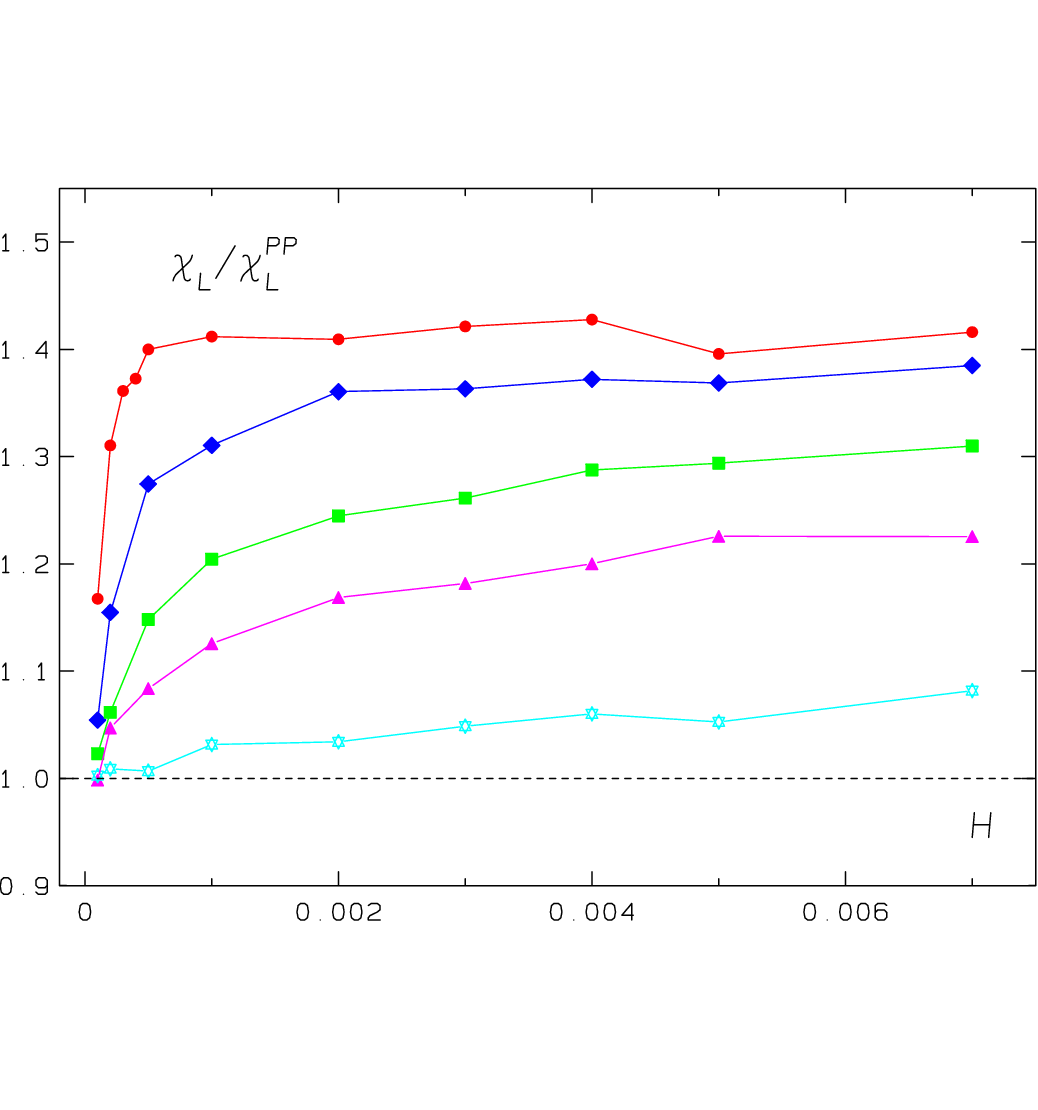
In Section 5.1 we have shown that the transverse correlators have the Gaussian form and we have determined the respective transverse masses . This enables us now to test the relation of Patashinskii and Pokrovskii which we have discussed in Section 2.4 . In Fig. 18 we plot the ratio of the measured longitudinal susceptibility to the result of Eq. (67) as a function of for all our couplings in the low temperature phase. As expected, the ratio is close to 1 for very small -values. For all couplings the ratio increases with increasing external field and reaches essentially a constant value. With decreasing temperature (increasing ) the ratio approaches 1 from above and at our lowest temperature we are for all -values already below 1.1 . The test of is of course a global one. More details are obtained from a direct comparison of the longitudinal correlator to its counterpart from Eq. (70). In Fig. 19 and 20 we show all our measured correlation functions for in the low temperature phase together with


the respective results from (70). In Fig. 19 we plot the correlators for and 0.95, the two couplings closest to the critical point. Whereas for the prediction from Eq. (70) is still definitely different from the data, the line and the data are close to each other already for , apart from the small -region. In Fig. 20 we observe with decreasing temperature a further approach, at the prediction coincides fully with the data. In the high temperature region the relation (50) obviously cannot hold for : there is no spontaneous magnetization and the longitudinal and transverse correlation functions must agree with each other. Accordingly, and can differ by a factor of for small external fields.
6.2 The stiffness
In Sections 2.4 and 3 we have discussed the behaviour of the stiffness . From our results for the transverse mass and the transverse susceptibility we can calculate using Eq. (51) . In Fig. 21 we show the stiffness as a function of (see Eq. (101) ) for fixed temperatures below . As expected, the stiffness increases with decreasing temperature. With decreasing external field the stiffness grows slightly, however for a finite value will be reached. This is different on the critical line, where
| (109) |
and is weakly diverging for . We have calculated the prefactor of from the critical parameters given in Ref. [3]. The prediction from the last equation is confirmed by our data as can be seen in Fig. 22. In the high temperature region


is close to one and only slowly varying with the external field. This is evident from Fig. 23, where we have plotted as a function of and not to avoid a too dense plot at small .

6.3 Scaling of the longitudinal correlation length
In Ref. [3] the scaling function of the longitudinal correlation length was calculated from the directly measured values of . For the longitudinal mass is the inverse of the longitudinal correlation length. Such an identification is not possible in the low temperature range where we have a whole continuum of contributing or -values. In the high temperature region however we can use the relation
| (110) |
to calculate the scaling function from our -data. The result is shown in Fig. 24 together with the asymptotic form for large -values from Eq. (96). Our data are scaling surprisingly well, better than the former results in Fig. 9 of Ref. [3], in particular in the small -region. One reason for the improvement may be the increase in the lattice size used, the other one is certainly the safer determination of as compared to that of . As in Ref. [3] we note the similarity in the form of this scaling function and that of the longitudinal susceptibility. Consequently, both functions peak at about the same value of , .

6.4 Magnetization and susceptibilities at
The behaviour of the magnetization and the susceptibilities and on the critical line is controlled by the critical exponent or rather its inverse as is evident from Eqs. (87) and (88). In Fig. 25 we show our data for at as a function of , where , the value of [3] was used. We compare the data with the result from Eq. (87) with , again from [3]. Except for the point at which perhaps shows some finite size effect, all data agree very well with the line. A straight line fit to the data for as a function of without the first point leads to a somewhat more accurate result
| (111) |
The ratio offers a straightforward way to determine : on the critical line it should coincide with the exponent. The drawback is however that the ratio has larger errors and that it shows definite finite size effects at small -values. The latter are due to the longitudinal susceptibility. In Fig. 26 we show our data for the ratio. The values for are still affected by the volume dependence. In order to determine we have therefore used only the points from . We find
| (112) |


7 Summary and conclusions
In our paper we have investigated the transverse and longitudinal 2-plane spin correlation functions of the three-dimensional O(4)-invariant non-linear -model. The data were obtained from simulations on a cubic lattice with linear extension for small external fields and temperatures below, above and at the critical temperature . The main objective was the determination of the spectral functions of the correlators. In particular we were interested in the identification of the lowest states of the spectra , which relate to the correlation lengthes by , the influence of possible higher states on the correlation functions, and the interplay of the transverse and longitudinal channels. In order to calculate the spectral functions we used Bryan’s algorithm for the maximum entropy method with a modified kernel which improves numerical stability at small .
As a result we find in the transverse case a single sharp peak in the spectral function for each of our and -values. The correlator is that of a free particle with mass , that is it has the known Gaussian form. We confirm therefore also corresponding assumptions of spin-wave theory about the dominance of long-wavelegth transverse fluctuations (i.e. small ) of Gaussian type for small fields below . In the very high temperature region we observe a single sharp peak as well in the longitudinal spectrum. On approaching the critical point from above the peak broadens somewhat and at its position coincides with for all our values. In the low temperature region we still find a significant peak at . At higher values a continuum of states with several peaks of decreasing heights appears. This is expected from a relation of Patashinskii and Pokrovskii between the longitudinal and the transverse correlation functions. However, a comparison of the relation with the correlation function data reveals that there must be additional contributions to the longitudinal spectra at higher external fields. With decreasing temperatures these additive contributions gradually disappear.
The influence of the longitudinal spin component on the transverse ones is characterized by the stiffness . As expected we find an increase of with decreasing temperature below . Above the critical temperature the stiffness is close to one and only weakly dependent on the external field. At we verify the predicted critical behaviour . With our results for for the high temperature region we have calculated the scaling function of the longitudinal correlation length. The new data scale surprisingly well, better than those of Ref. [3], which were derived from direct measurements of the correlation length. As a last check we have compared the data for the magnetization and the susceptibilities to the predicted critical behaviour at . We find again agreement with the former values and from [3]. A new fit to our data for the magnetization leads however to the more accurate numbers and .
Acknowledgments
We thank Frithjof Karsch for his suggestion to start this work and his constant interest. We are indebted to Olaf Kaczmarek for numerous stimulating discussions on the maximum entropy method and to Ines Wetzorke for the permission to use her MEM-program.
References
- [1] J. Zinn-Justin, Quantum Field Theory and Critical Phenomena, Clarendon Press, Oxford, 3rd Edition 1996.
- [2] R. Anishetty, R. Basu, N. D. Hari Dass and H. S. Sharatchandra, Int. J. Mod. Phys. A 14 (1999) 3467 [arXiv:hep-th/9502003].
- [3] J. Engels, L. Fromme and M. Seniuch, Nucl. Phys. B 675 (2003) 533 [arXiv:hep-lat/0307032].
- [4] M. E. Fisher and V. Privman, Phys. Rev. B 32 (1985) 447.
- [5] A. Z. Patashinskii and V. L. Pokrovskii, Zh. Eksp. Teor. Fiz. 64 (1973) 1445 [Sov. Phys. JETP 37 (1974) 733].
- [6] A. Cucchieri, J. Engels, S. Holtmann, T. Mendes and T. Schulze, J. Phys. A 35 (2002) 6517 [arXiv:cond-mat/0202017].
- [7] J. Engels, S. Holtmann and T. Schulze, PoS LAT2005 (2006) 148 [arXiv:hep-lat/0509010].
- [8] F. Basile, A. Pelissetto and E. Vicari, PoS LAT2005 (2006) 199 [arXiv:hep-lat/0509018].
- [9] S. Ejiri et al., arXiv:0909.5122 [hep-lat].
- [10] A. Z. Patashinskii and V. L. Pokrovskii, Fluctuation Theory of Phase Transitions, Pergamon, Oxford, 1979.
- [11] J. J. Binney, N. J. Dowrick, A. J. Fisher, and M. E. J. Newman, The Theory of Critical Phenomena, Clarendon Press, Oxford, 1992.
- [12] D. J. Wallace and R. K. P. Zia, Phys. Rev. B 12 (1975) 5340.
- [13] J. Engels, V. K. Mitrjushkin and T. Neuhaus, Nucl. Phys. B 440 (1995) 555 [arXiv:hep-lat/9412003].
- [14] M. Asakawa, T. Hatsuda and Y. Nakahara, Prog. Part. Nucl. Phys. 46 (2001) 459 [arXiv:hep-lat/0011040].
- [15] S. Datta, F. Karsch, P. Petreczky and I. Wetzorke, Phys. Rev. D 69 (2004) 094507 [arXiv:hep-lat/0312037].
- [16] G. Aarts, C. Allton, J. Foley, S. Hands and S. Kim, Phys. Rev. Lett. 99 (2007) 022002 [arXiv:hep-lat/0703008].
- [17] R. K. Bryan, Eur. Biophys. J. 18 (1990) 165.
- [18] Mark Jarrell, J. E. Gubernatis, Phys. Rep. 269 (1996) 133.
- [19] J. Engels, L. Fromme and M. Seniuch, Nucl. Phys. Proc. Suppl. 129 (2004) 783 [arXiv:hep-lat/0309005].
- [20] V. Privman, P. C. Hohenberg and A. Aharony, in Phase Transitions and Critical Phenomena, vol. 14, edited by C. Domb and J. L. Lebowitz (Academic Press, New York, 1991).
- [21] U. Wolff, Phys. Rev. Lett. 62 (1989) 361.
- [22] I. Dimitrovic, P. Hasenfratz, J. Nager and F. Niedermayer, Nucl. Phys. B 350 (1991) 893.
- [23] M. Oevers, Diploma thesis, Universität Bielefeld, 1996.