Simulating quantum computers with
probabilistic methods

In a first part of the paper, we develop tools to investigate weak classical simulation of QC. A central ingredient in our analysis will be a certain class of quantum states, called here computationally tractable states (CT states). Colloquially speaking, a state is CT if it is possible to classically simulate computational basis measurements on $|\psi\rangle$ and if the coefficients of $|\psi\rangle$ in this basis can be efficiently computed. As we will see, many important state families—matrix product states, stabilizer states, states generated by poly-size matchgate circuits, and several others—turn out to be CT. A second element will be the notion of efficiently computable sparse operators (ECS). An $n$-qubit operation is ECS if its matrix representation in the standard basis has at most poly$(n)$ nonzero entries per row and per column, and if these entries can be determined efficiently. For example, all Pauli products, $k$-local operators with $k=O(\log n)$, as well as operators that can be written as poly-size circuits of Toffoli gates, are ECS. We will prove the following result.

An immediate remark to be made is that the unitary operation $U$ itself is not required to be sparse—only its action on $O$ is to yield an ECS operation, which is a significantly distinct requirement. For example, if $U$ is a poly-size circuit consisting of nearest neighbor matchgates—which is generally not sparse at all—then $U^{\dagger}ZU$ is a linear combination of poly$(n)$ Pauli products, which is an ECS operation.

Theorem 1 identifies a general scenario in which quantum circuits can be simulated efficiently classically. This result turns out to be rather versatile and will be useful in a number of contexts. In this work we highlight the following particular applications (however, it is likely that this result has applications beyond the ones considered here):

• •

  Sparse circuits. A simple instance of theorem 1 is obtained by considering a product input state (which is trivially CT) and the $Z$ observable on, say, the first qubit, and by letting the circuit $U$ itself be an ECS operation (in which case $U^{\dagger}ZU$ is ECS as well). Then, by virtue of theorem 1, the resulting quantum computation can be simulated classically. In fact, one can immediately extend this result by composing $m$ efficiently computable $s$-sparse¹¹ 1 An operator is $s$-sparse if its standard basis matrix representation has at most $s$ nonzero entries per row and per column. unitary operations with $s^{m}=$ poly$(n)$. Then the overall circuit will still be ECS, as can easily be verified, and thus can be simulated classically due to theorem 1.

  Sparse unitary operations are of interest because they highlight the role of interference in quantum computation, as opposed to entanglement. In particular, sparse operations may produce highly entangled states but the interference exhibited in any sparse unitary evolution is always limited. As we will show, this absence of high degrees of interference can be exploited to construct an efficient classical simulation algorithm, in spite of the potentially complex entangled states produced throughout the computation. This provides (yet another) illustration that the presence of entanglement is by no means sufficient to guarantee quantum computational speed-ups. Sparse operations furthermore provide examples of a class of QCs where weak classical simulation is efficiently possible, whereas strong simulation is intractable ($\#$P-hard). In other words, adopting the notion of weak simulation constitutes a necessary ingredient in the simulation of sparse circuits whereas strong simulation methods such as e.g. tensor contraction schemes cannot (unless $\#$P $=$ P) yield an efficient classical simulation.

• •

  Composability. Instead of letting $|\psi\rangle$ be a simple product input state, we may also consider more complicated CT states which are e.g. the result of an earlier quantum computation, i.e. $|\psi\rangle=U^{\prime}|\psi_{\mbox{\scriptsize{in}}}\rangle$ for some simple (e.g. standard basis) input $|\psi_{\mbox{\scriptsize{in}}}\rangle$. As long as $|\psi\rangle$ is CT and subsequently a circuit $U$ is applied followed by measurement of $O$ such that $U^{\dagger}OU$ is ECS, the overall quantum circuit $UU^{\prime}$, acting on $|\psi_{\mbox{\scriptsize{in}}}\rangle$ and followed by measurement of $O$, can be simulated classically by theorem 1. One hence arrives at a criterion to asses when the concatenation of two quantum circuits can be simulated classically.

  

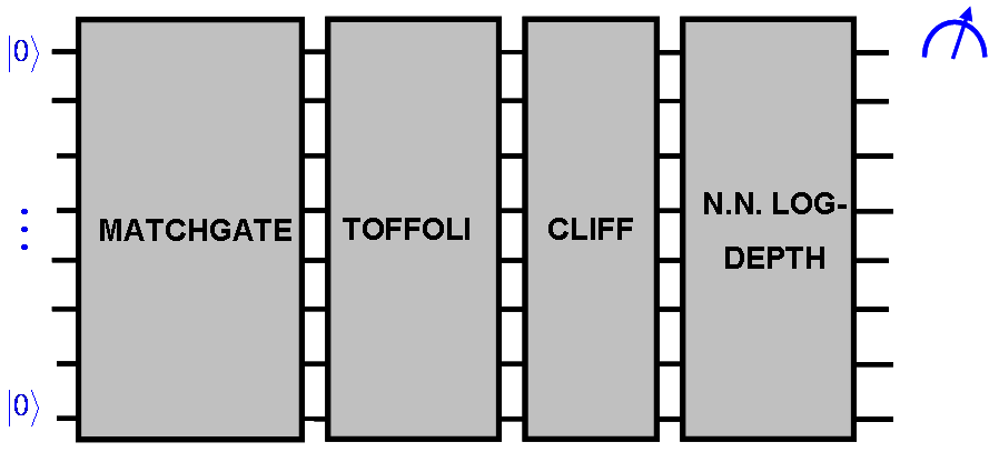
  Since the majority of existing efficiently simulatable circuits turn out to generate CT states when acting on suitable inputs and as at the same time many simulatable operations yield ECS operations when acting on suitable observables, the above composability result is applicable to a wide variety of settings. In particular, this result applies to Clifford operations, matchgate circuits, bounded-depth circuits, classical circuits, bounded-treewidth circuits, the quantum Fourier transform, and others. This leads to sometimes surprising examples of concatenated circuits that can be simulated classically (cf. Fig. 1). As illustrated in these examples, the concatenation of simulatable blocks of very different nature may remain efficiently simulatable classically (consider e.g. the concatenation of a Clifford with a matchgate circuit).

  It is interesting to compare the examples in Fig. 1 to powerful quantum algorithms such as Simon’s and Shor’s. Strikingly, the latter algorithms are implemented with particularly simple circuitry—arguably even simpler than the classically simulatable circuits displayed in Fig. 1. In particular, it is known that both the factoring algorithm and Simon’s algorithm can be efficiently implemented by a circuit with the very simple structure of Fig. 2 [16, 17]. Intriguingly, this circuit is the composition of only three blocks, each of which is elementary. Nevertheless, our simulation techniques cannot be successfully be applied to yield an efficient classical simulation of this circuit class. In the second part of this work we investigate the hardness of simulating these circuits and, by extension, Simon’s and Shor’s algorithms, in more detail.

• •

  CNOT-$e^{i\theta X}$ circuits. As a further application of theorem 1, we will show that poly-size circuits composed of CNOT and $e^{i\theta X}$ gates, acting on product inputs and followed by measurement of $Z$ on any single qubit, can be simulated classically. This result is of interest since it is known that CNOT together with any single real one-qubit gate $V$ such that $V^{2}$ is not basis-preserving, is universal for quantum computation [18]. In contrast to this, here it is found that there is a class of non-trivial complex gates $e^{i\theta X}$ that can be added to the CNOT gate while retaining efficient classical simulation.

  The above result is also interesting from a conceptual point of view. In particular, its proof will follow from a variant of theorem 1 where states $|\psi\rangle$ and operations $U^{\dagger}OU$ are considered that are CT, resp. ECS, with respect to bases other than the standard basis. Letting $|\psi\rangle$ be a product input and $U$ a poly-size circuit composed of CNOT and $e^{i\theta X}$ gates, it will be shown that $|\psi\rangle$ and $U^{\dagger}Z_{1}U$ are CT, resp. ECS, with respect tho the $\{|\pm\rangle\}$ basis of $X$ eigenstates. Hence, viewing the entire computation in this basis and applying theorem 1 shows that classical simulation is efficiently possible. In contrast, a direct application of theorem 1, i.e. with respect to the standard basis, is not possible as $U^{\dagger}Z_{1}U$ is generally not ECS w.r.t this basis.

In a second part of the paper, the above results are applied in the context of quantum algorithms. Depending on the case at hand, the goal will be to either show that certain algorithms can be simulated classically or to deepen our insight into why certain algorithms achieve exponential (oracle) speed-ups over classical computation. We will analyze three different quantum algorithms:

• •

  a quantum algorithm to estimate partition functions of classical lattice models [19];

• •

  a general class of quantum algorithms containing the Deutsch-Jozsa algorithm [20];

• •

  Simon’s algorithm [17].

The first two classes of quantum algorithms will be proved to be classically simulatable using the methods developed in this paper. We refer to the relevant sections in the text for a discussion. For the time being, we limit ourselves to discussing our results in the context of Simon’s algorithm, which we consider the most interesting application.

Recall that in Simon’s problem one has oracle access to a function $f:\{0,1\}^{n}\to\{0,1\}^{n}$; it is promised that there exists an unknown $n$-bit string $a$ such that $f(x)=f(y)$ if and only if $y=x+a$ (addition modulo 2). The goal is to find $a$. Classically one needs at least $O(2^{\frac{n}{2}})$ queries, whereas a quantum computer can solve the problem with $O(n)$ queries—i.e. Simon’s algorithm achieves an exponential oracle separation between BQP and BPP. In spite of its computational power, Simon’s algorithm is implemented with very simple circuitry, as displayed in Fig. 2. What are the essential ingredients responsible for the power of this algorithm?

In standard considerations, the interplay between the Fourier transform (i.e. the second layer of Hadamards in Fig. 2) and the oracle $f$ is emphasized. After the oracle is applied, the system is in the state $\sum|x\rangle|f(x)\rangle$. The Fourier transform then creates interference in the system and “picks out” the relevant computational basis states, such that a subsequent measurement of the system yields the desired information about the unknown bit-string $a$. This rather delicate relation between oracle and Fourier transform is usually considered to be among the main origins of the hardness of classically simulating Simon’s algorithm. In this work we will show that this point of view is not the end of the story: in particular, we will find that the interplay between the same Fourier transform and the function computed during the round of classical postprocessing is an equally important element in the speed-up achieved by the algorithm. Specifically, we will prove the following result.

Thus, if the final classical round in Simon’s algorithm happened to regard a function with sufficiently peaked fourier spectrum, then the entire quantum computation could be simulated efficiently —independent of the details of e.g. the oracle $f$ computed in an earlier stage of the computation, and independent of e.g. the entanglement produced by the quantum circuit. This result hence exposes the double role played by the Fourier transform, which is to act appropriately on both the oracle $f$ and the function computed in the postprocessing, in order to achieve a quantum speed-up. These observations highlight that the power of a quantum algorithm can only be understood by taking the entire computation into account including the classical postprocessing round, even though the latter may at first sight look rather innocuous. Indeed, note that—strikingly—in Simon’s algorithm this round ‘only’ involves solving a simple system of linear equations over $\mathbb{Z}_{2}$! Nevertheless, this simple classical computation is associated with a function having a very flat spectrum (as we will see), hence ensuring the exponential speed up achieved by Simon’s algorithm.

Remark: in the formulation of theorem 2, no knowledge of the Fourier spectrum of the function in question is assumed, except the promise that this spectrum is “peaked”. Using remarkable results of Boolean learning theory, enough information of the spectrum can be efficiently reconstructed in order to achieve the poly-time classical simulation as stated in the theorem. $\diamond$

Finally, also the factoring algorithm can be implemented with a circuit displaying the structure of Fig. 2. Therefore, the classical postprocessing plays a similar crucial role also in this algorithm. As the technical considerations in Simon’s algorithm are more transparent than in Shor’s, here we will focus on the former—keeping in mind that our conclusions also apply to the latter.

Somewhat unrelated to the above context, we prove a “byproduct result” that we find noteworthy. We will arrive at a complexity-theoretic result regarding the computational power of matchgate circuits. Roughly speaking, we will show the following (see theorem 4 for a precise statement):

• The class of functions that can be efficiently computed by nearest-neighbor matchgate circuits is strictly contained within P.

Perhaps the most interesting aspect regarding this result here is its proof method. Surprisingly, the result will be obtained by combining the classical query lower bound of Simon’s problem with our theorem 1. In particular, we will show that if the class of matchgate-computable functions comprised all of P, then a quantum algorithm for Simon’s problem would exist which turns out to be efficiently simulatable classically (using theorem 1). Hence an efficient classical algorithm would exist which solves Simon’s problem with poly$(n)$ classical oracle queries, yielding a contradiction. Remark that it is striking how utterly unrelated matchgate circuits and Simon’s problem seem at first sight!

Throughout this paper, we will deal with $n$-qubit state families $\{|\psi_{n}\rangle:n=1,2,\dots\}$, where $|\psi_{n}\rangle$ is an $n$-qubit state. When considering such a state family $\{|\psi_{n}\rangle\}$, we will mostly refer to a single state $|\psi_{n}\rangle\equiv|\psi\rangle$ with the silent assumption that this actually denotes a family. We now consider the following definition.

For convenience, in (b) we require the coefficients $\langle x|\psi\rangle$ to be computable with perfect precision, a notion which may lead to rather pathological situations when e.g. irrational numbers are involved. The results in this paper can however straightforwardly be generalized to the case where $\langle x|\psi\rangle$ can be computed efficiently with exponential precision, i.e. up to $m$ significant bits in poly$(n,m)$ time. As in the present work the distinction between these two types of accuracies is not essential (in contrast to the distinction between polynomial and exponential precision, which is crucial), for clarity we state all results w.r.t. the notion of perfect accuracy. Also in other places in the text where we refer to ‘perfect accuracy’, the results in question immediately generalize to the case of exponential precision.

Note that (a) and (b) are highly dependent on the classical description of the state $|\psi\rangle$ that is provided. Therefore, strictly speaking it would be more precise to call a state $|\psi\rangle$ CT relative to this classical description. In this paper we will only encounter situations where each state has a natural (efficient) description that will be obvious from the context. It will always be assumed that this particular description is provided. For example, the classical description of a state generated by a poly-size quantum circuit acting on, say, the all-zeroes input, will always be assumed to be the circuit that generates the state. As another example, for every complete product state $|\psi\rangle=|\psi_{1}\rangle\otimes\dots\otimes|\psi_{n}\rangle$ we will assume $|\psi\rangle$ to be specified in terms of the ‘obvious’ description of $|\psi\rangle$ consisting if the $2n$ complex coefficients $\langle 0|\psi_{i}\rangle$ and $\langle 1|\psi_{i}\rangle$.

Even though conditions (a) and (b) are similar in nature, we provide evidence that these conditions are incomparable. In particular, the following complexity theoretic argument implies that it is highly likely that there exists states satisfying (b) but not (a). Consider any efficiently computable function $f:\{0,1\}^{n}\to\{0,1\}$ for which it is promised that there exists a unique $x_{0}$ such that $f(x_{0})=1$, and define the $n$-qubit state $|\psi\rangle=\sum_{x}f(x)|x\rangle=|x_{0}\rangle$. Note that the state $|\psi\rangle$ satisfies condition (b). Assuming that (b) implies (a), it follows that it is possible to efficiently sample from the distribution $\{|\langle x|\psi\rangle|^{2}\}$. But this distribution assigns a zero probability to each bit string $x$ except $x_{0}$, which has unit probability. Hence, the possibility of efficiently sampling from this distribution implies that $x_{0}$ can be determined efficiently. Regarding $f$ as a verifier circuit for an NP problem, it would immediately follow that every problem in NP with a unique witness is in P. This last property is not likely to be true [21].

Next we state a useful sufficient (but not necessary) criterion to assess whether condition (a) holds for a given state. To state this result, we need the following notation. For an $n$-qubit state $|\psi\rangle$, let $p_{S,y}(|\psi\rangle)\equiv p_{S,y}$ denote the probability of obtaining the bit string $y=(y_{i}:i\in S)$ as an outcome when measuring the qubits in the set $S\subseteq\{1,\dots,n\}$. We can then state the following lemma; a proof can be found in e.g. [11].

Several important state families turn out to be computationally tractable, as illustrated next.

• •

  Examples of computationally tractable states:

• –

  Product states are trivially CT.

• –

  Every state of the form $|\psi\rangle\propto\sum_{x}e^{i\theta(x)}|x\rangle$, where the sum is over all $n$-bit strings $x$ and where $x\to\theta(x)\in\mathbb{R}$ represents an arbitrary efficiently computable function, is trivially CT. Every state obtained by applying a poly-size circuit family consisting of Toffoli gates to an arbitrary product state is computationally tractable as well, as can easily be proved (this property will also follow from lemma 2).

• –

  Every matrix product state (MPS) of polynomial bond dimension is CT. A state $|\psi\rangle$ is an MPS of poly bond dimension if there exist $2n$ $N\times N$ matrices $A_{i}[0],A_{i}[1]$ with $N=$ poly$(n)$ such that $\langle x|\psi\rangle$ $=$ $\mbox{ Tr}(A_{1}[x_{1}]\dots A_{n}[x_{n}])$, for every $n$-bit string $x=(x_{1},\dots,x_{n})$. Property (b) follows immediately from this definition. Property (a) holds since the conditions of lemma 1 are satisfied for all MPS of polynomial bond dimension [22]. Tree tensor states [23] are generalizations of MPS with similar properties and are also computationally tractable.

• –

  A Clifford circuit is a quantum circuit composed of Hadamard, CNOT and PHASE gates, where PHASE $=$ diag$(1,i)$. An $n$-qubit stabilizer state is any state that is generated by applying a poly-size Clifford circuit to the state $|0\rangle^{n}$. Every stabilizer state is a CT state. Property (a) is the content of the Gottesman-Knill theorem [6]. Property (b) is proved in [7] (see also [10]).

• –

  A (unitary, two-qubit) matchgate $G$ is any two-qubit gate of the form

  $\displaystyle G=\left[\begin{array}[]{cccc}a&&&b\\ &u&v&\\ &x&y&\\ c&&&d\end{array}\right],\quad A=\left[\begin{array}[]{cc}a&b\\ c&d\end{array}\right],\quad B=\left[\begin{array}[]{cc}u&v\\ x&y\end{array}\right],$

  where $A,B\in SU(2)$. Every state obtained by applying a poly-size matchgate circuit to a computational basis state, where all gates are restricted to act on nearest neighbors (assuming a one-dimensional ordering of the qubits) is a computationally tractable state. Properties (a) and (b) are proved in [11].

• –

  Any $n$-qubit state that is obtained by applying the quantum Fourier transform (over the integers modulo $2^{n}$) to an arbitrary product state, is a CT state. See e.g. [24] for a simple proof of this property (see also [25, 26] for related results).

• –

  We briefly mention a general class of classical simulation results related to efficient tensor contraction schemes. This approach relies on the topology of (a graph associated with) the quantum circuit in question. If this topology displays a sufficiently tree-like structure (quantified in terms of the graph invariant tree-width) then classical simulation of such circuits can be achieved [27]. It can be shown that the output states of quantum circuits with logarithmically scaling tree-width (acting on product input states), are CT states; the proof essentially contained in [27] and is omitted here (see also [4] for related work).

Next we investigate which operations map the family of CT states to itself. In this context, the operations that preserve the computational basis play an important role. An $n$-qubit operation $M$ is called ‘basis-preserving’ if every computational basis state $|x\rangle$ is mapped to $M|x\rangle=\gamma_{x}|{\pi(x)}\rangle$, for some permutation $\pi$ of the set of $n$-bit strings and some complex $\gamma_{x}$. The operation $M$ is efficiently computable if the functions $x\to\gamma_{x}$, $x\to\pi(x)$ and $x\to\pi^{-1}(x)$ can be evaluated in poly$(n)$ time. For example, every Pauli product [28] is efficiently computable basis-preserving, as well as every operation of the form $O=\sum_{x}(-1)^{f(x)}|x\rangle\langle x|$, where $f:\{0,1\}^{n}\to\{0,1\}$ is an efficiently computable function. Also every poly-size circuit composed of elementary basis-preserving gates (e.g. Toffoli gates, diagonal gates) is efficiently computable basis-preserving.

The relevance of efficiently computable basis-preserving unitary operations in the present context is that these operations preserve the class of CT states:

Proof: Let the permutation $\pi$ and the coefficients $\gamma_{x}$ be defined as above. Note that $|\gamma_{x}|=1$ for every $x$ since $M$ is unitary. The coefficients of $|\psi^{\prime}\rangle$ are given by $\langle x|\psi^{\prime}\rangle=\gamma_{\pi^{-1}(x)}\langle{\pi^{-1}(x)}|\psi\rangle$. Property (b) now follows immediately from the properties that $M$ is efficiently computable and that $|\psi\rangle$ is CT. To show (a), we have to find an efficient classical method to sample from the probability distribution defined by Prob$(x)=|\langle x|\psi^{\prime}\rangle|^{2}=|\langle{\pi^{-1}(x)}|\psi\rangle|^{2}$. To do so, consider the following procedure. First sample from the distribution $\{|\langle y|\psi\rangle|^{2}\}$, yielding a bit string $y$ with probability $|\langle y|\psi\rangle|^{2}$, and subsequently output the bit string $x:=\pi(y)$. This procedure is efficient since $|\psi\rangle$ is CT and $y\to\pi(y)$ is efficiently computable. Moreover, every bit string $x$ is generated with probability $|\langle{\pi^{-1}(x)}|\psi\rangle|^{2}$ as desired. $\square$

Note that the basis-preserving operation $M$ may drastically change the entanglement properties of $|\psi\rangle$. Consider e.g. the case where $|\psi\rangle$ is a complete product state and $M$ a poly-size circuit of CPHASE and/or Toffoli operations, yielding a state $|\psi^{\prime}\rangle$ that may be highly entangled. Nevertheless, both $|\psi\rangle$ and $|\psi^{\prime}\rangle$ are CT and equal up to a basis-preserving operation.

Next we consider sparse operations. Such operations are sufficiently close to basis-preserving operations that their action on CT states remains manageable. An $n$-qubit operation $A$ is $s$-sparse if for every basis state $|x\rangle$, each of the vectors $A|x\rangle$ and $A^{T}|x\rangle$ is a linear combination of at most $s$ computational basis states. The quantity $s$ is called the sparseness of $A$. We will consider $n$-qubit operations $A$ (both unitary operations and observables) with sparseness $s\leq$ poly$(n)$, which will simply be called ‘sparse operations’. Note that the notion of sparseness is defined w.r.t. to the number of nonzero entries per row/column and not the total number of nonzero entries in the matrix, the latter not being required to be small. In particular, a sparse $n$-qubit operation generically has a total number of nonzero entries that scales exponentially with $n$.

For every $s$-sparse $n$-qubit operation $A$, define $2s$ functions $\alpha_{i}:\{0,1\}^{n}\to\mathbb{C}$ and $r_{i}:\{0,1\}^{n}\to\{0,1\}^{n}$ ($i=1,\dots,s$) as follows: the $n$-bit string $r_{i}(x)$ is defined to be the row index of $A$ associated with the $i$-th non-zero entry in the column indexed by $x$ (when traversing this column from top to bottom), if an $i$-th nonzero entry exists within this column; we denote this entry by $\alpha_{i}(x)$. If an $i$-th nonzero entry does not exist in this column, then $r_{i}(x)$ is set to be the all-zeroes string and $\alpha_{i}(x)$ is set to zero. With the above definitions, one simply has

Similar definitions can be given regarding the rows of $A$, leading to $2s$ functions $\beta_{i}:\{0,1\}^{n}\to\mathbb{C}$ and $c_{i}:\{0,1\}^{n}\to\{0,1\}^{n}$ ($i=1,\dots,s$) that are the natural counterparts of the $\alpha_{i}$ and $r_{i}$, respectively.

A sparse $n$-qubit operation $A$ is efficiently column-computable if, on input of an arbitrary $n$-bit string $x$, it is possible to list the (at most $s=$ poly$(n)$) nonzero entries within the column of $A$ indexed by $x$ together with the row indices associated with each of these non-zero entries, all in poly$(n)$ time. Equivalently, $A$ is efficiently column-computable if it is possible to compute the $2s$ quantities $\alpha_{i}(x)$ and $r_{i}(x)$ ($i=1,\dots,s$) in poly-time. The operation $A$ is called efficiently row-computable if $A^{T}$ is efficiently column-computable. Finally, $A$ is called efficiently computable if it is both efficiently row- and column-computable. All efficiently computable sparse unitary operations can be implemented efficiently on a quantum computer [29]. In this paper we will only consider sparse operations that are efficiently computable.

The following are some examples of efficiently computable sparse operations.

• •

  Examples of efficiently computable sparse (ECS) operations:

• –

  Every efficiently computable basis-preserving operation is ECS.

• –

  Every $d$-qubit gate $G$ acting within an $n$-qubit circuit, represented by the matrix $G\otimes I$ where $I$ denotes the identity acting on $n-d$ qubits, is $2^{d}$-sparse. If $d=O(\log n)$ then such an operation is ECS.

• –

  Every operation that is a linear combination of poly$(n)$ ECS operations, is ECS. It follows that every operator $H=\sum_{i=1}^{m}H_{i}$ which is a sum of $m=$ poly$(n)$ $d$-local observables $O_{i}$ (with $d=O(\log n)$) is ECS. This means that observables such as Hamiltonians and correlation operators are typically ECS.

• –

  Let $U$ represent an $n$-qubit poly-size circuit of basis-preserving elementary gates (e.g. Toffoli, CNOT, PHASE, CPHASE, etc.), interspersed with $k$ gates $V_{1},\dots,V_{k}$ at arbitrary places in the circuit, each of which acts on at most $d$ qubits. It is required that $kd=O(\log n)$; otherwise the $V_{i}$ are arbitrary. Then $U$ is ECS. To see this, expand each gate $V_{i}$ as a linear combination of $4^{d}$ Pauli products and note that every Pauli product is efficiently computable basis-preserving. Consequently, $U$ can be written as a linear combination of $4^{dk}=$ poly$(n)$ efficiently computable basis-preserving operations, showing that $U$ is ECS.

• –

  ECS operations often arise in the context of quantum algorithms, related e.g. to unitary group representations; see e.g. [29] and references within.

We are now in a position to state the following result, which constitutes the main technical ingredient in this work regarding the use of sampling techniques in classical simulation.

Note that theorem 1 immediately follows from theorem 3. Before proving this result in its most general form, as a warm-up we prove a special instance, taking $A$ to be the identity. Hence, we are concerned with the estimation of overlaps between CT states. This special case is proved beforehand to illustrate the sampling methods used in this work, without the more technically involved arguments required in the proof of theorem 3. Thus, we set out to prove the following property, formulated in terms of a lemma.

Proof: Denote $p_{x}:=|\langle x|\psi\rangle|^{2}$ and $q_{x}:=|\langle x|\varphi\rangle|^{2}$. Since $|\psi\rangle$ and $|\varphi\rangle$ are CT states, it is possible to sample efficiently from the probability distributions $\{p_{x}\}$ and $\{q_{x}\}$. Define the function $\delta:\{0,1\}^{n}\to\{0,1\}$ by $\delta(x)=1$ if $p_{x}\geq q_{x}$ and $\delta(x)=0$ otherwise, for every $n$-bit string $x$, and define $\epsilon=1-\delta$. Then $\delta$ and $\epsilon$ can be evaluated efficiently since $p_{x}$ and $q_{x}$ can be efficiently evaluated by assumption (b) in the definition of CT states. The overlap $\langle\varphi|\psi\rangle$ is therefore equal to

where the sums are over all $n$-bit strings $x$. Defining the functions $F$ and $G$ by

we have $\langle\varphi|\psi\rangle=\langle F\rangle+\langle G\rangle$ where $\langle F\rangle=\sum p_{x}F(x)$ and $\langle G\rangle=\sum q_{x}G(x)$. It follows from assumption (b) in the definition of CT states that $F$ and $G$ can be efficiently evaluated. Furthermore, both $|F(x)|$ and $|G(x)|$ are not greater than 1. It thus follows from the Chernoff-Hoeffding bound that both $\langle F\rangle$ and $\langle G\rangle$ can be approximated efficiently with polynomial accuracy. This implies that $\langle\varphi|\psi\rangle$ can be estimated with polynomial accuracy as well. This completes the proof. $\square$

Lemma 3 shows that the overlap $\langle\varphi|\psi\rangle$, representing a ‘joint’ property of the states $|\psi\rangle$ and $|\varphi\rangle$, may be estimated efficiently classically even when only an efficient simulation of quantum processes resulting in $|\psi\rangle$ and $|\varphi\rangle$ individually is available—in particular, the techniques leading to the proofs of (a)-(b) (cf. definition of CT states) for $|\psi\rangle$ and $|\varphi\rangle$, may be completely different. For example, the overlap between a matrix product state and a stabilizer state can be estimated efficiently classically with polynomial accuracy, even though such states are CT due to very different argumentations.

We are now in a position to prove theorem 3.

Proof of theorem 3: It is sufficient to prove the result for CT states $|\psi\rangle$ and $|\varphi\rangle$. Let $s=$ poly$(n)$ denote the sparseness of $A$. Using the notation of (10), we have $\langle\varphi|A|\psi\rangle=\sum_{i=1}^{n}\sigma_{i}$, where we denote

Note that $|\alpha_{i}(x)|\leq 1$. It is sufficient to prove that each of the $s$ quantities $\sigma_{i}$ can be estimated efficiently with polynomial accuracy, for then also $\sum_{i=1}^{s}\sigma_{i}$ can be estimated with polynomial accuracy as $s=$ poly$(n)$. To do so, write $p_{x}:=|\langle x|\psi\rangle|^{2}$ and $q_{x}:=|\langle x|\varphi\rangle|^{2}$. Define a function $\delta_{i}$ by $\delta_{i}(x)=1$ if $p_{x}\geq q_{r_{i}(x)}$ and $\delta_{i}(x)=0$ otherwise, for every $n$-bit string $x$, and define $\epsilon_{i}=1-\delta_{i}$. Then $\delta_{i}$ and $\epsilon_{i}$ can be evaluated efficiently since $|\psi\rangle$ and $|\varphi\rangle$ are CT and $A$ is ECS. We split $\sigma_{i}$ in two parts by inserting $\delta_{i}(x)+\epsilon_{i}(x)=1$:

The function $F_{i}$ defined by

is efficiently computable and satisfies $|F_{i}(x)|\leq 1$ for every $x$. The first term in the r.h.s. of (14) is hence equal to $\langle F_{i}\rangle=\sum p_{x}F_{i}(x)$, which can be estimated to polynomial accuracy efficiently due to the Chernoff-Hoeffding bound. To estimate the second term in the r.h.s. of (14), one needs to be careful since the function $r_{i}$ may not be injective. We proceed as follows. Define the following function $G_{i}$:

with the additional convention that $G_{i}(y)$ is zero if there are no $x$ such that $r_{i}(x)=y$ and $\alpha_{i}(x)\neq 0$. With this definition, the second term in the r.h.s. of (14) is equal to $\langle G_{i}\rangle=\sum_{y}q_{y}G_{i}(y)$. We now make the following claims. Claim 1: the function $G_{i}$ is efficiently computable; and Claim 2: $|G_{i}(y)|\leq s$ for every $y$. A proof of claims 1 and 2 implies that $\langle G_{i}\rangle$ can be estimated in poly-time with polynomial accuracy due to the Chernoff-Hoeffding bound. But then also $\sigma_{i}$ can be estimated efficiently, thus completing the proof.

We now prove Claim 1. Since $A$ is $s$-sparse, every row $y$ has at most $s$ non-zero entries. Equivalently, the following set contains at most $s$ strings $x$:

Hence, a fortiori, for every fixed $i$ there are at most $s$ different $x$ such that $r_{i}(x)=y$ and $\alpha_{i}(x)\neq 0$. Moreover, given an arbitrary $y$ it is possible to efficiently determine all these $x$’s and the corresponding coefficients $\alpha_{i}(x)$. This is done in two steps: first, since $A$ is efficiently (row-)computable, given a row index $y$ it is possible to compute all (at most $s$) strings $x$ in the set (17) in poly-time; second, for all those $x$ one computes $r_{i}(x)$ and $\alpha_{i}(x)$—this is possible in poly-time since $A$ is efficiently column-computable—and verifies whether $r_{i}(x)$ is equal to $y$; those $x$ for which $r_{i}(x)=y$ are kept, the others discarded.

It follows that $G_{i}(y)$ is a sum of at most $s=$ poly$(n)$ terms, each of which is efficiently computable. Thus, Claim 1 is proved. Moreover, Claim 2 now immediately follows as well, since the modulus of every term in the sum (16) is smaller than one and there are at most $s$ terms in the sum. This proves theorem 3. $\square$

Remark: poly-ECS operations.— In the definition of ECS operations and in the subsequent statement of theorem 3, we have required that the non-zero entries of $A$ can be computed efficiently with perfect precision. Theorem 3 also holds for sparse operations where, instead, these coefficients can be estimated efficiently with polynomial accuracy, which is a significant relaxation. Call an $n$-qubit operation $A$ $(\|A\|\leq 1)$ poly-ECS if it is sparse, and if (i) on input of an arbitrary column index $x$, it is possible to determine in poly-time all those row indices $y$ such that $\langle y|A|x\rangle\neq 0$ and if the corresponding nonzero entries $\langle y|A|x\rangle$ can be estimated in poly-time with polynomial accuracy, and (ii) similarly for the row indices $y$. Theorem 3 then also holds for poly-ECS operations. The proof is completely analogous to the above proof of theorem 3. The only difference is that now the functions $F_{i}(x)$ and $G_{i}(x)$ can no longer be computed exactly, but only with polynomial accuracy. However, this suffices to invoke the Chernoff-Hoeffding bound (cf. the Appendix). This remark will play an important role in the discussion of Simon’s algorithm i.e. in the proof of theorem 2. $\diamond$

We conclude this section with two corollaries of theorem 3. Corollary 1 shows that expectation values of local observables can be estimated efficiently classically for every CT state. This result may potentially be of use in e.g. variational Monte Carlo studies of strongly correlated systems (this is work in progress). Corollary 2 will be of use when we discuss the Deutsch-Jozsa algorithm in section 6.2.

Proof: this result follows immediately from theorem 3 since every $d$-local $O$ with $d=O(\log n)$ is ECS. Here we provide a short alternative proof that does not require the formalism used in the proof of theorem 3. Every observable $O$ of the form considered can be written as a linear combination of $N=$ poly$(n)$ Pauli operators: $O=\sum_{i=1}^{N}a_{i}P_{i}$, with $|a_{i}|\leq 1$. Consequently,

As each $P_{i}$ is an efficiently computable basis-preserving unitary operation, each state $P_{i}|\psi\rangle$ is CT due to lemma 2. Invoking lemma 3, the overlap between $P_{i}|\psi\rangle$ and $|\psi\rangle$ can be estimated classically with polynomial accuracy. Hence, also $\langle O\rangle$ can be estimated classically with polynomial accuracy. This proves the result. $\square$

Proof: The proof uses a technique related to the SWAP test. Denote $|\psi^{\prime}\rangle:=B|\psi\rangle$ and $|\varphi^{\prime}\rangle:=A^{\dagger}|\varphi\rangle$ (which are potentially unnormalized states) and consider the following identity:

where the unitary operator $U_{\mbox{\scriptsize{SWAP}}}$ swaps qubit $i$ with qubit $i+k$, for every $i=1,\dots,k$. The identity (19) can easily be verified. Hence, we have

Note that the $(k+n)$-qubit states $|\xi\rangle|\psi\rangle$ and $|\chi\rangle|\varphi\rangle$ are CT. Moreover, it can easily be verified that $U_{\mbox{\scriptsize{SWAP}}}$ is ECS. This implies that the operation $[I\otimes A]U_{\mbox{\scriptsize{SWAP}}}[I\otimes B]$ is ECS as well, being a product of three ECS operations. Theorem 3 can now be applied. $\square$

Note that, as a special case of this last result, it follows that partial overlaps $\langle\varphi|[|\xi\rangle\langle\chi|\otimes I]|\psi\rangle$ between CT states can be estimated efficiently classically.

The following is a formal statement of the classical simulation of sparse circuits which was announced in the introduction.

Proof: Let $|\psi\rangle$ denote the product input state and let $Z_{1}$ denote the $Z$ observable acting on the first qubit. The expectation value of $Z_{1}$ is given by $\langle Z_{1}\rangle=\langle\psi|U^{\dagger}ZU|\psi\rangle$. Note that $U$ is ECS due to the restrictions on $s$ and $m$; but then also the observable $O:=U^{\dagger}ZU$ is ECS, being a product of three ECS operations. Moreover, $|\psi\rangle$ is a product state and hence CT. Theorem 1 can now be applied. $\square$

As briefly alluded to in the introduction, sparse operations highlight the role of interference—as opposed to entanglement—in quantum computation. Note that sparse operations may generically produce highly entangled states. Consider e.g. the simple case where the input is $|+\rangle^{n}$ and the entire circuit $U$ is composed of poly$(n)$ CPHASE gates (which are basis-preserving gates and thus particularly simple examples of sparse operations). With such circuits, it is possible to efficiently generate e.g. the highly entangled cluster states [30]. On the other hand, if a sparse operation $U$ acts on a state $|\psi\rangle$ then each coefficient of $U|\psi\rangle$ in the standard basis is a linear combination of at most poly$(n)$ coefficients of $|\psi\rangle$. Hence, the “interference” in the process $|\psi\rangle\to U|\psi\rangle$ is limited (we use the notion of interference in a colloquial sense and do not adopt any technical definition). Corollary 3 states that quantum computational processes where the interference is “small” in this sense, cannot offer any speed-up compared to classical computers, in spite of the high degrees of entanglement that may be generated throughout the computation. Corollary 3 may thus be regarded as complementary to a class of results stating that quantum computations that generate low amounts of entanglement (quantified appropriately) can be classically simulated efficiently (see e.g. [1, 2, 3, 4, 5]).

Finally, note that in corollary 3 one cannot hope for an improvement of the bound $s^{m}=$ poly$(n)$ to e.g. $m=$ poly$(n)$ and $s$ constant (unless BQP = BPP) since every poly-size quantum circuit is a product of $m=$ poly$(n)$ single- and two-qubit gates, each of which is an $s$-sparse operation with $s$ constant.

Theorem 1 immediately leads to a criterion to assess when the composition of two quantum circuits can be simulated classically. Formally, we have:

Next we provide some illustrations of this result. First we provide some examples of pairs $(U,O)$ such that $U^{\dagger}OU$ is ECS. All circuit families $U$ below are poly-size.

• •

  Examples of pairs $(U,O)$ where $U^{\dagger}OU$ is ECS:

• –

  Let $U$ be a circuit of constant depth and let the observable $O$ act nontrivially on $O(\log n)$ qubits. Then $U^{\dagger}OU$ also acts nontrivially on $O(\log n)$ qubits and is hence an ECS observable.

• –

  Let $U$ represent a Clifford circuit and let $O$ be any observable that is a linear combination of $N=$ poly$(n)$ Pauli products: $O=\sum_{i=1}^{N}a_{i}P^{i}$ with $|a_{i}|\leq 1$ and $P^{i}$ Pauli operators. Then $U^{\dagger}OU$ is again a linear combination of $N$ Pauli products, and hence ECS.

• –

  Let $U$ be a circuit composed of nearest-neighbor matchgates and let $Z_{1}$ denote the Pauli $Z$ operation acting on the first qubit. Then $U$ maps $Z_{1}$ (under conjugation) to a linear combination of poly$(n)$ Pauli products (see e.g. [14]), which is an ECS operation.

Next we explicitly describe two concatenated circuits that can be simulated efficiently using our results; see also Fig 1. In both examples, the circuit acts on the all-zeroes computational basis state and is followed by measurement of $Z$ on the first qubit.

• •

  Examples of corollary 4:

• –

  Consider a quantum circuit $V=V_{4}V_{3}V_{2}V_{1}$ where $V_{1}$ is an arbitrary local unitary operation, $V_{2}$ represents the quantum Fourier transform (over $\mathbb{Z}_{2^{n}}$), $V_{3}$ is an arbitrary efficiently computable sparse unitary, and $V_{4}$ is an arbitrary poly-size (nearest-neighbor) matchgate circuit. Then this circuit can be simulated efficiently classically due to corollary 4. In particular, we show that corollary 4 can be applied by taking $U_{1}\equiv V_{2}V_{1}$ and $U_{2}\equiv V_{4}V_{3}$. To see this, note first that $V_{2}V_{1}$ acting on the input yields a CT state. Further, $(V_{4}V_{3})^{\dagger}Z(V_{4}V_{3})$ is ECS: indeed, $V_{4}^{\dagger}ZV_{4}$ is a sum of poly$(n)$ Pauli products and hence ECS, and thus $(V_{4}V_{3})^{\dagger}Z(V_{4}V_{3})$ is ECS as well, being a product of three ECS operations. Corollary 4 can now be applied.

• –

  Consider a quantum circuit $V=V_{4}V_{3}V_{2}V_{1}$ where $V_{1}$ is an arbitrary poly-size matchgate circuit, $V_{2}$ is a poly-size circuit of Toffoli gates, $V_{3}$ is an arbitrary poly-size Clifford circuit and $V_{4}$ is an arbitrary log-depth circuit consisting of nearest-neighbor gates. We show that corollary 4 can be applied by taking $U_{1}\equiv V_{1}$ and $U_{2}\equiv V_{4}V_{3}V_{2}$. To see this, note first that $V_{1}$ acting on the input yields a CT state. Further, $(V_{4}V_{3}V_{2})^{\dagger}Z(V_{4}V_{3}V_{2})$ is ECS: $V_{4}^{\dagger}ZV_{4}$ acts nontrivially on $O(\log n)$ qubits and is hence is a linear combination of poly$(n)$ Pauli products; but then also $V_{3}^{\dagger}V_{4}^{\dagger}ZV_{4}V_{3}$ is a linear combination of poly$(n)$ Pauli products (and hence ECS) since $V_{3}$ is a Clifford operation; finally, it follows that $(V_{4}V_{3}V_{2})^{\dagger}Z(V_{4}V_{3}V_{2})$ is ECS as this operation is a product of three ECS operations. Corollary 4 thus again yields the desired result.

Several other examples of the above nature can easily be generated.

In our definition of computationally tractable states and sparse operations, as well as in the resulting theorem 1, we have singled out a particular basis—i.e. the computational basis. Note, however, that in the vast majority of all arguments we have never relied on the specific form of this basis. Therefore, we may consider a generalized definition of CT states, sparse operations, etc., stated relative to a arbitrary basis ${\cal B}$, and carry out an analogous program as done so far, leading a much broader class of results. Results such as theorem 1 can be transferred in an obvious way, and will be omitted. Here we limit ourselves to discussing an example that can be understood using this generalized notion of CT states. This example regards the simulation of circuits composed of CNOTs and $e^{i\theta X}$ gates. Other examples of similar nature can easily be constructed.

Let ${\cal B}=\{|b_{x}\rangle\}$ denote the $|\pm\rangle$ product basis, defined by $|b_{x}\rangle\propto\bigotimes_{i=1}^{n}[|0\rangle+(-1)^{x_{i}}|1\rangle]$ for every $n$-bit string $x=(x_{1},\dots,x_{n})$. A state is called ‘computationally tractable in the basis ${\cal B}$’ if it is possible to sample in poly$(n)$ time with classical means from the probability distribution Prob$(x)=|\langle b_{x}|\psi\rangle|^{2}$, and if the coefficients $\langle b_{x}|\psi\rangle$ can be computed in poly$(n)$ time classically. It is clear that $|\psi\rangle$ is CT in ${\cal B}$ iff $H^{\otimes n}|\psi\rangle$ is CT in the computational basis. For example, it can easily be shown that every stabilizer state, as well as any MPS $|\psi\rangle$ is computationally tractable in the $|\pm\rangle$-basis ${\cal B}$ as $H^{\otimes n}|\psi\rangle$ is in both cases CT in the computational basis.

Similarly, the notion of ECS operations w.r.t. ${\cal B}$ is defined in the natural way. Obviously, $A$ is ECS w.r.t. ${\cal B}$ iff $H^{\otimes n}AH^{\otimes n}$ is ECS in the computational basis. For example, let $U$ denote an arbitrary poly-size $n$-qubit circuit composed of CNOT and $e^{i\theta X}$ gates, where $\theta$ may be any (real) angle. Whereas $U$ is generally not ECS in the computational basis, this circuit is always ECS in the $|\pm\rangle$ basis ${\cal B}$. This can be seen as follows. Let CNOT_ab denote a CNOT gate with control $a$ and target $b$. One then has the pair of identities

both of which are easily verified. These identities imply that $M:=H^{\otimes n}UH^{\otimes n}$ is a poly-size circuit consisting entirely of CNOT and $e^{i\theta Z}$ gates and is thus ECS (even basis-preserving) in the computational basis. This shows that $U$ is ECS in the $|\pm\rangle$ product basis.

One can now consider a generalized form of theorem 1, now stated relative to the $|\pm\rangle$ basis (or any other basis):

• Theorem 1’ Let $|\psi_{\mbox{\scriptsize{in}}}\rangle$ be an $n$-qubit state, let $U$ denote a poly-size $n$-qubit circuit and let $O$ denote an observable. If $|\psi\rangle$ is CT in ${\cal B}$ and if $U^{\dagger}OU$ is ECS in ${\cal B}$, then the circuit $U$, acting on $|\psi_{\mbox{\scriptsize{in}}}\rangle$ and followed by measurement of $O$, can be simulated efficiently classically.

Now consider a CNOT-$e^{i\theta X}$ circuit $U$ as above. The circuit $U$ acts on an arbitrary product input $|\alpha\rangle$ and is followed by measurement of $Z_{1}$. We now claim that this computation can be simulated efficiently classically, using the above variant of theorem 1. To see this, first note that $|\alpha\rangle$ is CT in ${\cal B}$. Second, $O:=U^{\dagger}Z_{1}U$ is ECS in ${\cal B}$: to show this, note that $H^{\otimes n}OH^{\otimes n}=M^{\dagger}X_{1}M.$ Here, as before, $M:=H^{\otimes n}U_{2}H^{\otimes n}$ is a poly-size circuit consisting entirely of CNOT and $e^{i\theta Z}$ gates, and $X_{1}$ denotes the Pauli $X$ operation acting on the first qubit. The operation $M^{\dagger}X_{1}M$ is basis-preserving in the computational basis, hence $O=H^{\otimes n}[M^{\dagger}X_{1}M]H^{\otimes n}$ is basis-preserving in ${\cal B}$. This proves the claim; note that we have hence proved:

Here we point out that a recently proposed quantum algorithm [19], concerned with estimating partition functions of classical spin systems such as the Potts model, can be simulated efficiently classically. Letting ${\cal Z}$ denote the Potts model partition function defined on some (arbitrary) lattice, the quantum algorithm in [19] provides a polynomial approximation of the quantity ${\cal Z}/\Delta$. Here $\Delta$ denotes a particular, easy-to-compute normalization factor that depends on the couplings of the model (see [19], Cor. 5.9, for the precise form of $\Delta$); $\Delta$ is sometimes called the ‘approximation scale’ of the algorithm. On the other hand, in [31] mappings were established which allow to express the same quantity ${\cal Z}/\Delta$ as the overlap between a suitable product state $|\alpha\rangle$ and stabilizer state $|\psi\rangle$: ${\cal Z}/{\Delta}=\langle\alpha|\psi\rangle$. Note that both stabilizer states and product states are CT (see section 4). Using theorem 3 (in fact: the special instance $A=I$ of lemma 3, dealing with overlaps between CT states), we find that overlaps between stabilizer states and product states can also efficiently be estimated with polynomial accuracy with classical methods. Hence, the quantity ${\cal Z}/{\Delta}$ can also be estimated with polynomial accuracy in poly-time using classical means, showing that the quantum algorithm in question can be simulated efficiently classically.

We emphasize that the work [19] contains several quantum algorithms besides the partition function algorithm focused on here (in particular, the latter does not constitute the main result of [19]), including algorithms for BQP-complete problems, to which our classical simulation techniques do not apply.

An application of corollary 2 is found by considering the Deutsch-Jozsa (DJ) algorithm [20]. Recall that in the DJ problem one considers a black-box function $f:\{0,1\}^{n}\to\{0,1\}$ which is promised to be either constant or balanced [32]. The task is to determine which possibility holds. Classically, any deterministic solution to the problem requires exponentially many oracle calls, whereas a randomized classical algorithm can solve the DJ problem with exponentially small probability of failure using $O(n)$ queries. The DJ quantum algorithm constitutes a deterministic solution to the problem using a single query of the oracle.

Thus, it is well known that DJ can be simulated classically when an exponentially small probability of failure is allowed. Here we will reproduce this result, showing that it immediately follows from corollary 2. Moreover, we will find that a large class of generalizations (to be specified below) can be efficiently simulated as well. The argument is very general and mainly regards the structure of the involved circuits.

Going through the steps in the DJ algorithm, it is easily verified that DJ is implemented by a circuit belonging to the following general class (the system is initialized in the state $|0\rangle^{n}$):

• Round 1: apply a local unitary operation $V_{1}$;

  Round 2: apply an ECS operation $V_{2}$;

  Round 3: apply another local unitary operation $V_{3}$ ;

  Round 4: measure the observable $O=|0\rangle\langle 0|^{k}\otimes I$, for some $k\leq n$.

Using corollary 2, we now immediately find that such a computation can be simulated efficiently classically. Indeed, the state obtained after Round 1 is a a product state and hence CT. Moreover, the operation in round 2 is efficiently computable sparse. Finally, the observable $O^{\prime}:=V_{3}^{\dagger}OV_{3}$ has the form $|\gamma\rangle\langle\gamma|\otimes I$ for some $k$-qubit product—and hence CT—state $|\gamma\rangle$. Corollary 2 can now immediately be applied.

Note that, in the argument, the specific form of the function $f$ (computed in Round 2) is completely irrelevant. This shows that the lack in computational power of the DJ algorithm is a structural feature of the circuit. In particular, this computational weakness cannot be overcome by e.g. changing the form of the oracle, but must involve a more drastic alteration of the circuit structure.

Lastly, we consider Simon’s algorithm [17]. As this algorithm has the admirable feature of being a very simple quantum algorithm that nevertheless achieves an exponential speed-up, it is an ideal candidate to compare quantum and classical computational power. Simon’s algorithm is worth investigating from a number of angles. As a comprehensive study would lead us too far, here we single out one particular aspect, namely the surpising role of the round of classical postprocessing in the algorithm taking place after the measurement. We will show that this seemingly innocuous round of classical computation plays a rather determining role in the performance of the algorithm.

References

- [1] R. Jozsa and N. Linden, arXiv:quant-ph/0201143 (2002).
- [2] G. Vidal, Phys. Rev. Lett. 91, 147902 (2003).
- [3] N. Yoran and A. Short, quant-ph/0601178 (2006).
- [4] R. Jozsa, arXiv:quant-ph/0603163 (2006).
- [5] M. Van den Nest, W. Dür, G. Vidal and H. J. Briegel, Phys. Rev. A 75, 012337 (2007).
- [6] D. Gottesman, talk at International Conference on Group Theoretic Methods in Physics, arXiv:quant-ph/9807006 (1998).
- [7] J. Dehaene and B. De Moor, Phys. Rev. A 68, 042318 (2003).
- [8] S. Aaronson and D. Gottesman, Phys. Rev. A 70:052328 (2004).
- [9] S. Clark, R. Jozsa, N. Linden, arXiv:quant-ph/0701103 (2007).
- [10] M. Van den Nest, arXiv:0811.0898 (2008).
- [11] L. G. Valiant, SIAM J. Comput. 31, No. 4, p. 1229 (2002).
- [12] D. DiVincenzo and B. Terhal, Phys. Rev. A 65, 032325/1-10 (2002).
- [13] S. Bravyi, Cont. Math., Vol. 482, pp. 179-211 (2009).
- [14] R. Jozsa and A. Miyake, Proc. R. Soc. A 464, 3089-3106 (2008).
- [15] R. Jozsa, B. Kraus, A. Miyake, J. Watrous, arXiv:0908.1467 (2009).
- [16] A. Y. Kitaev, quant-ph/9511026 (1995).
- [17] D. Simon, SIAM J. Computing 26, 1474-1483 (1997).
- [18] Y. Shi, arXiv:quant-ph/0205115 (2002).
- [19] I. Arad and Z. Landau, arXiv:0805.0040 (2008).
- [20] D. Deutsch and R. Jozsa (1992), Proc. Roy. Soc. A 439: 553 (1992).
- [21] L. G. Valiant and V. V. Vazirani, ACM Press New York, NY, USA (1985).
- [22] D. Perez-Garcia, F. Verstraete, M.M. Wolf, J.I. Cirac, Quantum Inf. Comput. 7, 401 (2007).
- [23] Y. Shi, L.-M. Duan and G. Vidal, Phys. Rev. A 74, 022320 (2006).
- [24] D. E. Browne, New J. Phys. 9 146 (2007).
- [25] N. Yoran and A. Short, Phys. Rev. A 76, 042321 (2007).
- [26] D. Aharonov, Z. Landau and J. Makowsky, quant-ph/0611156 (2006).
- [27] I. Markov and Y. Shi, SIAM J. Comp., 38(3):963-981 (2008).
- [28] Recall that an -qubit Pauli operator (or Pauli product) has the form , where each is either the identity or one of the Pauli matrices , or .
- [29] S. P. Jordan and P. Wocjan, arXiv:0904.2211 (2009).
- [30] M. Hein et al., In Proceedings of the International School of Physics ‘Enrico Fermi’ on ‘Quantum Computers, Algorithms and Chaos’ (2005); arXiv:quant-ph/0602096.
- [31] M. Van den Nest, W. Dür and H. J. Briegel, Phys. Rev. Lett. 98, 117207 (2007).
- [32] A function is constant if for every -bit string ; is balanced if exactly inputs satisfy .
- [33] Y. Mansour, Theoretical Advances in Neural Computation and Learning, 391-424, Kluwer Academic Publishers (1994).
- [34] A. Bernasconi and B. Codenotti, IEEE Trans. Computers 48, 3, 345351 (1999).
- [35] The converse, however, is not true. For example, there exist degree-2 polynomials with sparseness (the inner product function is an example of this).
- [36] E. Kushilevitz and Y. Mansour, SICOMP 22(6): 1331-1348 (1993).
- [37] That is, and , for every matrix .
- [38] R. A. Horn and C. R. Johnson, Matrix Analysis, Cambridge Univ. Press (1990).
- [39] We remark that in the definition of , in the most general case one must allow to use poly ancillary qubits prepared in, say, the state , i.e. . For clarity, we have not incorporated this in the proof; the argument can be generalized appropriately without significant complications.