跳到论文正文
W Papers独立论文阅读器 arXiv:0911.1464 论文正文 计算阅读时间 · 0%
引用这篇论文根据当前论文元数据生成,正式投稿前建议核对。


License: arXiv.org perpetual non-exclusive license
arXiv:0911.1464v2 [hep-ex] 10 Nov 2009

UCHEP-09-03 𝑫𝟎D^{0}-𝑫¯ 0\overline{D}{}^{\,0} Mixing and 𝑪​𝑷CP Violation: HFAG Combination of Parameters

A. J. Schwartz
(representing the HFAG charm group)
††thanks: alan.j.schwartz@uc.edu Affiliation: Physics Department, University of Cincinnati, Cincinnati, OH 45221, USA
Abstract

We present the most recent set of world averages for D0D^{0}-D¯ 0\overline{D}{}^{\,0} mixing and C​PCP violation parameters, as obtained by the Heavy Flavor Averaging Group from a global fit to various measurements. The values obtained for the mixing parameters when allowing for C​PCP violation are x=(0.98−0.26+0.24)%x=(0.98\,^{+0.24}_{-0.26})\% and y=(0.83±0.16)%y=(0.83\,\pm 0.16)\%; the significance of mixing is 10.2​σ10.2\sigma. There is no evidence for C​PCP violation at the current level of sensitivity.

1 Introduction

In 2006, the Heavy Flavor Averaging Group (HFAG) [1] convened a new subgroup to calculate world average (WA) values of charm mixing and C​PCP violation (C​P​VCPV) parameters [2]. Since that time, D0D^{0}-D¯ 0\overline{D}{}^{\,0} mixing has been observed, and a wealth of mixing and C​P​VCPV results have appeared. The HFAG charm group has calculated several sets of WA values, updating old averages as new results have become available. This paper presents the most recent set of averages, i.e., those based on results that appeared in preprint form by the summer of 2009.

Mixing in the B0B^{0} and Bs0B^{0}_{s} heavy flavor systems is governed by the short-distance box diagram. In the D0D^{0} system, however, this diagram is doubly-Cabibbo-suppressed (relative to amplitudes dominating the decay width) and also GIM-suppressed. Thus, the short-distance mixing rate is tiny, and D0D^{0}-D¯ 0\overline{D}{}^{\,0} mixing is expected to be dominated by long-distance processes. These are difficult to calculate reliably, and theoretical estimates for D0D^{0}-D¯ 0\overline{D}{}^{\,0} mixing range over 2-3 orders of magnitude [3, 4].

The decay rates for D0→fD^{0}\!\rightarrow\!f and D¯ 0→f¯\overline{D}{}^{\,0}\!\rightarrow\!\bar{f} are, respectively,

d​ND0d​t\displaystyle\frac{dN_{D^{0}}}{dt} ∝\displaystyle\!\!\propto\!\! e−Γ¯​t{R++|qp|R+×\displaystyle e^{-\overline{\Gamma}\,t}\ \left\{R^{+}+\left|\frac{q}{p}\right|\sqrt{R^{+}}\,\times\right. (1)
(y′​cos⁡ϕ−x′​sin⁡ϕ)​(Γ¯​t)+\displaystyle\hskip 28.90755pt(y^{\prime}\cos\phi-x^{\prime}\sin\phi)(\overline{\Gamma}t)+
|qp|2(x′2+y′2)4(Γ¯t)2}\displaystyle\hskip 50.58878pt\left.\left|\frac{q}{p}\right|^{2}\frac{(x^{\prime 2}+y^{\prime 2})}{4}(\overline{\Gamma}\,t)^{2}\right\}
dND¯ 0d​t\displaystyle\frac{dN_{\overline{D}{}^{\,0}}}{dt} ∝\displaystyle\!\!\propto\!\! e−Γ¯​t{R−+|pq|R−×\displaystyle e^{-\overline{\Gamma}\,t}\ \left\{R^{-}+\left|\frac{p}{q}\right|\sqrt{R^{-}}\,\times\right. (2)
(y′​cos⁡ϕ+x′​sin⁡ϕ)​(Γ¯​t)+\displaystyle\hskip 28.90755pt(y^{\prime}\cos\phi+x^{\prime}\sin\phi)(\overline{\Gamma}t)+
|pq|2(x′2+y′2)4(Γ¯t)2}.\displaystyle\hskip 50.58878pt\left.\left|\frac{p}{q}\right|^{2}\frac{(x^{\prime 2}+y^{\prime 2})}{4}(\overline{\Gamma}\,t)^{2}\right\}\!.

In these expressions, x′=x​cos⁡δ+y​sin⁡δx^{\prime}=x\cos\delta+y\sin\delta and y′=y​cos⁡δ−x​sin⁡δy^{\prime}=y\cos\delta-x\sin\delta, where x=(M2−M1)/Γ¯x=(M_{2}-M_{1})/\overline{\Gamma} and y=(Γ2−Γ1)/(2​Γ¯)y=(\Gamma_{2}-\Gamma_{1})/(2\overline{\Gamma}) are mixing parameters, and δ\delta is the strong phase difference between amplitudes 𝒜(D¯→ 0f){\cal A}(\overline{D}{}^{\,0}\!\rightarrow\!f) and 𝒜⁡(D0→f){\cal A}(D^{0}\!\rightarrow\!f). Parameters M1M_{1}, M2M_{2}, Γ1\Gamma_{1}, and Γ2\Gamma_{2} are the masses and decay widths of the mass eigenstates |D1⟩≡p|D0⟩+q|D¯⟩ 0|D_{1}\rangle\equiv p|D^{0}\rangle+q|\overline{D}{}^{\,0}\rangle and |D2⟩≡p|D0⟩−q|D¯⟩ 0|D_{2}\rangle\equiv p|D^{0}\rangle-q|\overline{D}{}^{\,0}\rangle, and Γ¯=(Γ1+Γ2)/2\overline{\Gamma}=(\Gamma_{1}+\Gamma_{2})/2. Our convention is CP|D0⟩=−|D¯⟩ 0CP|D^{0}\rangle=-|\overline{D}{}^{\,0}\rangle such that for q=pq\!=\!p, D1D_{1} is C​PCP-odd and D2D_{2} is C​PCP-even. The parameters R+=|𝒜(D0→f)/𝒜(D¯→ 0f)|2R^{+}=|{\cal A}(D^{0}\!\rightarrow\!f)/{\cal A}(\overline{D}{}^{\,0}\!\rightarrow\!f)|^{2}, R−=|𝒜(D¯→ 0f¯)/𝒜(D0→f¯)|2R^{-}=|{\cal A}(\overline{D}{}^{\,0}\!\rightarrow\!\bar{f})/{\cal A}(D^{0}\!\rightarrow\!\bar{f})|^{2}, and ϕ=Arg⁡(q/p)\phi={\rm Arg}(q/p).

To obtain WA values of x,y,δ,|q/p|x,y,\delta,|q/p|, and ϕ\phi, we perform a global fit to 28 measured observables. These observables are from measurements of D0→K+​ℓ−​νD^{0}\!\rightarrow\!K^{+}\ell^{-}\nu, D0→K+​K−/π+​π−D^{0}\!\rightarrow\!K^{+}K^{-}/\pi^{+}\pi^{-}, D0→K+​π−D^{0}\!\rightarrow\!K^{+}\pi^{-}, D0→K+​π−​π0D^{0}\!\rightarrow\!K^{+}\pi^{-}\pi^{0}, D0→KS0​π+​π−D^{0}\!\rightarrow\!K^{0}_{S}\,\pi^{+}\pi^{-}, and D0→K+​K−​KS0D^{0}\!\rightarrow\!K^{+}K^{-}K^{0}_{S} decays [5], and from double-tagged branching fractions measured in e+​e−→ψ⁡(3770)→D​De^{+}e^{-}\!\rightarrow\!\psi(3770)\!\rightarrow\!DD reactions. To fit these observables, we must include an additional strong phase δK​π​π\delta_{K\pi\pi} (see below). For D0→K+​π−D^{0}\!\rightarrow\!K^{+}\pi^{-} decays, we combine R+R^{+} and R−R^{-} into parameters RD≡(R++R−)/2R_{D}\equiv(R^{+}+R^{-})/2 and AD≡(R+−R−)/(R++R−)A_{D}\equiv(R^{+}-R^{-})/(R^{+}+R^{-}). Correlations among observables are accounted for by using covariance matrices provided by the experimental collaborations.

With the exception of the ψ⁡(3770)→D​D\psi(3770)\!\rightarrow\!DD measurements, all methods identify the flavor of the D0D^{0} or D¯ 0\overline{D}{}^{\,0} when produced by reconstructing the decay D∗⁣+→D0​π+D^{*+}\!\rightarrow\!D^{0}\pi^{+} or D∗⁣−→D¯​π− 0D^{*-}\!\rightarrow\!\overline{D}{}^{\,0}\pi^{-}; the charge of the accompanying pion identifies the DD flavor. For signal decays, MD∗−MD0−Mπ+≡Q≈6M_{D^{*}}-M_{D^{0}}-M_{\pi^{+}}\equiv Q\approx 6 MeV, which is relatively close to the threshold. Thus, analyses typically require that the reconstructed QQ be small to suppress backgrounds. For time-dependent measurements, the D0D^{0} decay time is calculated as (ℓ/p)×MD0(\ell/p)\times M_{D^{0}}, where ℓ\ell is the distance between the D∗D^{*} and D0D^{0} decay vertices and pp is the D0D^{0} momentum. The D∗D^{*} vertex position is taken to be either the primary vertex position (p¯​p\bar{p}p experiments) or else is calculated from the intersection of the D0D^{0} momentum vector with the beam-spot profile (e+​e−e^{+}e^{-} experiments).

2 Input Observables

The global fit determines central values and errors for x,y,δ,RD,AD,|q/p|,ϕx,\,y,\,\delta,\,R_{D},A_{D},\,|q/p|,\,\phi, and δK​π​π\delta_{K\pi\pi} using a χ2\chi^{2} statistic. Parameters xx and yy govern mixing, and parameters ADA_{D}, |q/p||q/p|, and ϕ\phi govern C​P​VCPV. The parameter δK​π​π\delta_{K\pi\pi} is the strong phase difference between amplitudes 𝒜(D¯→ 0K+π−π0){\cal A}(\overline{D}{}^{\,0}\!\rightarrow\!K^{+}\pi^{-}\pi^{0}) and 𝒜⁡(D0→K+​π−​π0){\cal A}(D^{0}\!\rightarrow\!K^{+}\pi^{-}\pi^{0}) evaluated at MK+​π−=MK∗​(890)M_{K^{+}\pi^{-}}=M_{K^{*}(890)}.

All input values are listed in Table 1. The values for observables RM=(x2+y2)/2R_{M}=(x^{2}+y^{2})/2 [6], yC​Py_{CP} [7], and AΓA_{\Gamma} [7] are HFAG WA values [8]. They are calculated as weighted averages of measurements, taking into account correlations among systematic errors and sometimes also statistical errors. As an example, the weighted average for yC​Py_{CP} is shown in Fig. 1. The values of observables from D0→KS0​π+​π−D^{0}\!\rightarrow\!K^{0}_{S}\,\pi^{+}\pi^{-} decays [9] for no-C​P​VCPV are HFAG WA values [8], but for the C​P​VCPV-allowed case only Belle measurements are available. The D0→K+​π−D^{0}\!\rightarrow\!K^{+}\pi^{-} results used [10] are from Belle, Babar, and CDF, as these results have much greater precision than earlier ones. The D0→K+​π−​π0D^{0}\!\rightarrow\!K^{+}\pi^{-}\pi^{0} results are from Babar [11], and the ψ⁡(3770)→D​D\psi(3770)\!\rightarrow\!DD results are from CLEOc [12].

Table 1: Input values used for the global fit, from Refs. [6, 7, 9, 10, 11, 12].
Observable Value Comment
yC​Py_{CP}
AΓA_{\Gamma}
(1.107±0.217)%(0.123±0.248)%\begin{array}[]{c}(1.107\pm 0.217)\%\\ (0.123\pm 0.248)\%\end{array}
WA D0→K+​K−/π+​π−D^{0}\!\rightarrow\!K^{+}K^{-}/\pi^{+}\pi^{-} and D0→K+​K−​KS0D^{0}\!\rightarrow\!K^{+}K^{-}K^{0}_{S} results [8]
xx (no C​P​VCPV)
yy (no C​P​VCPV)
|q/p||q/p| (no direct C​P​VCPV)
ϕ\phi (no direct C​P​VCPV)
(0.811±0.334)%(0.811\pm 0.334)\%
(0.309±0.281)%(0.309\pm 0.281)\%
0.95±0.22−0.09+0.100.95\pm 0.22^{+0.10}_{-0.09}
(−0.035±0.19±0.09)(-0.035\pm 0.19\pm 0.09) rad
No C​P​VCPV:
WA D0→KS0​π+​π−D^{0}\!\rightarrow\!K^{0}_{S}\,\pi^{+}\pi^{-} results [8]
xx
yy
|q/p||q/p|
ϕ\phi
(0.81±0.30−0.17+0.13)%(0.81\pm 0.30^{+0.13}_{-0.17})\%
(0.37±0.25−0.15+0.10)%(0.37\pm 0.25^{+0.10}_{-0.15})\%
0.86±0.30−0.09+0.100.86\pm 0.30^{+0.10}_{-0.09}
(−0.244±0.31±0.09)(-0.244\pm 0.31\pm 0.09) rad
C​P​VCPV-allowed:
Belle D0→KS0​π+​π−D^{0}\!\rightarrow\!K^{0}_{S}\,\pi^{+}\pi^{-} results. Correlation coefficients:
      {1−0.007−0.255​α0.216−0.0071−0.019​α−0.280−0.255​α−0.019​α1−0.128​α0.216−0.280−0.128​α1}\left\{\begin{array}[]{cccc}1&-0.007&-0.255\alpha&0.216\\ -0.007&1&-0.019\alpha&-0.280\\ -0.255\alpha&-0.019\alpha&1&-0.128\alpha\\ 0.216&-0.280&-0.128\alpha&1\end{array}\right\}
Note: α=(|q/p|+1)2/2\alpha=(|q/p|+1)^{2}/2 is a variable transformation factor
RMR_{M} (0.0130±0.0269)%(0.0130\pm 0.0269)\% WA D0→K+​ℓ−​νD^{0}\!\rightarrow\!K^{+}\ell^{-}\nu results [8]
x′′x^{\prime\prime}
y′′y^{\prime\prime}
(2.61−0.68+0.57±0.39)%(2.61\,^{+0.57}_{-0.68}\,\pm 0.39)\%
(−0.06−0.64+0.55±0.34)%(-0.06\,^{+0.55}_{-0.64}\,\pm 0.34)\%
Babar D0→K+​π−​π0D^{0}\!\rightarrow\!K^{+}\pi^{-}\pi^{0} result. Correlation coefficient =−0.75=-0.75.
Note: x′′≡xcosδK​π​π+ysinδK​π​πx^{\prime\prime}\equiv x\cos\delta_{K\pi\pi}+y\sin\delta_{K\pi\pi}, y′′≡ycosδK​π​π−xsinδK​π​πy^{\prime\prime}\equiv y\cos\delta_{K\pi\pi}-x\sin\delta_{K\pi\pi}.
RMR_{M}
yy
RDR_{D}
RD​cos⁡δ\sqrt{R_{D}}\cos\delta
(0.199±0.173±0.0)%(0.199\pm 0.173\pm 0.0)\%
(−5.207±5.571±2.737)%(-5.207\pm 5.571\pm 2.737)\%
(−2.395±1.739±0.938)%(-2.395\pm 1.739\pm 0.938)\%
(8.878±3.369±1.579)%(8.878\pm 3.369\pm 1.579)\%
CLEOc results from “double-tagged” branching fractions
measured in ψ⁡(3770)→D​D\psi(3770)\!\rightarrow\!DD decays. Correlation coefficients:
      {1−0.06440.00720.0607−0.06441−0.3172−0.83310.0072−0.317210.38930.0607−0.83310.38931}\left\{\begin{array}[]{cccc}1&-0.0644&0.0072&0.0607\\ -0.0644&1&-0.3172&-0.8331\\ 0.0072&-0.3172&1&0.3893\\ 0.0607&-0.8331&0.3893&1\end{array}\right\}
Note: the only external input to these fit results are
branching fractions.
RDR_{D}
x′2+x^{\prime 2+}
y′⁣+y^{\prime+}
(0.303±0.0189)%(0.303\pm 0.0189)\%
(−0.024±0.052)%(-0.024\pm 0.052)\%
(0.98±0.78)%(0.98\pm 0.78)\%
Babar D0→K+​π−D^{0}\!\rightarrow\!K^{+}\pi^{-} results. Correlation coefficients:
      {10.77−0.870.771−0.94−0.87−0.941}\left\{\begin{array}[]{ccc}1&0.77&-0.87\\ 0.77&1&-0.94\\ -0.87&-0.94&1\end{array}\right\}
ADA_{D}
x′2−x^{\prime 2-}
y′⁣−y^{\prime-}
(−2.1±5.4)%(-2.1\pm 5.4)\%
(−0.020±0.050)%(-0.020\pm 0.050)\%
(0.96±0.75)%(0.96\pm 0.75)\%
Babar D0→K+​π−D^{0}\!\rightarrow\!K^{+}\pi^{-} results; correlation coefficients same as above.
RDR_{D}
x′2+x^{\prime 2+}
y′⁣+y^{\prime+}
(0.364±0.018)%(0.364\pm 0.018)\%
(0.032±0.037)%(0.032\pm 0.037)\%
(−0.12±0.58)%(-0.12\pm 0.58)\%
Belle D0→K+​π−D^{0}\!\rightarrow\!K^{+}\pi^{-} results. Correlation coefficients:
      {10.655−0.8340.6551−0.909−0.834−0.9091}\left\{\begin{array}[]{ccc}1&0.655&-0.834\\ 0.655&1&-0.909\\ -0.834&-0.909&1\end{array}\right\}
ADA_{D}
x′2−x^{\prime 2-}
y′⁣−y^{\prime-}
(2.3±4.7)%(2.3\pm 4.7)\%
(0.006±0.034)%(0.006\pm 0.034)\%
(0.20±0.54)%(0.20\pm 0.54)\%
Belle D0→K+​π−D^{0}\!\rightarrow\!K^{+}\pi^{-} results; correlation coefficients same as above.
RDR_{D}
x′2x^{\prime 2}
y′y^{\prime}
(0.304±0.055)%(0.304\pm 0.055)\%
(−0.012±0.035)%(-0.012\pm 0.035)\%
(0.85±0.76)%(0.85\pm 0.76)\%
CDF D0→K+​π−D^{0}\!\rightarrow\!K^{+}\pi^{-} results. Correlation coefficients:
      {10.923−0.9710.9231−0.984−0.971−0.9841}\left\{\begin{array}[]{ccc}1&0.923&-0.971\\ 0.923&1&-0.984\\ -0.971&-0.984&1\end{array}\right\}
Refer to caption
Figure 1: WA value of yC​Py_{CP} as calculated from D0→K+​K−D^{0}\!\rightarrow\!K^{+}K^{-}, D0→π+​π−D^{0}\!\rightarrow\!\pi^{+}\pi^{-}, and D0→K+​K−​KS0D^{0}\!\rightarrow\!K^{+}K^{-}K^{0}_{S} measurements [7].

The relationships between the observables and the fitted parameters are listed in Table 2. For each set of correlated observables, we construct a difference vector V→\vec{V}. For example, V→=(Δ​x,Δ​y,Δ​|q/p|,Δ​ϕ)\vec{V}=(\Delta x,\Delta y,\Delta|q/p|,\Delta\phi) for D0→KS0​π+​π−D^{0}\!\rightarrow\!K^{0}_{S}\,\pi^{+}\pi^{-} decays, where Δ\Delta represents the difference between the measured value and the fitted parameter value. The contribution of a set of observables to the χ2\chi^{2} is calculated as V→⋅(M−1)⋅V→T\vec{V}\cdot(M^{-1})\cdot\vec{V}^{T}, where M−1M^{-1} is the inverse of the covariance matrix for the measurement. All covariance matrices used are listed in Table 1.

Table 2: Left: decay modes used to determine the parameters x,y,δ,RD,AD,|q/p|,ϕx,\,y,\,\delta,\,R_{D},\,A_{D},\,|q/p|,\,\phi, and δK​π​π\delta_{K\pi\pi}. Middle: observables measured for each decay mode. Right: the relationships between the observables and the fitted parameters.
Decay Mode Observables Relationship
D0→K+​K−/π+​π−/K+​K−​KS0D^{0}\!\rightarrow\!K^{+}K^{-}/\pi^{+}\pi^{-}/K^{+}K^{-}K^{0}_{S}
yC​Py_{CP}
AΓA_{\Gamma}
2​yC​P=(|q/p|+|p/q|)​y​cos⁡ϕ−(|q/p|−|p/q|)​x​sin⁡ϕ2​AΓ=(|q/p|−|p/q|)​y​cos⁡ϕ−(|q/p|+|p/q|)​x​sin⁡ϕ\begin{array}[]{c}2y_{CP}=\left(\left|q/p\right|+\left|p/q\right|\right)y\cos\phi\ -\ \left(\left|q/p\right|-\left|p/q\right|\right)x\sin\phi\\ 2A_{\Gamma}=\left(\left|q/p\right|-\left|p/q\right|\right)y\cos\phi\ -\ \left(\left|q/p\right|+\left|p/q\right|\right)x\sin\phi\end{array}
D0→KS0​π+​π−D^{0}\!\rightarrow\!K^{0}_{S}\,\pi^{+}\pi^{-} xy|q/p|ϕ\begin{array}[]{c}x\\ y\\ |q/p|\\ \phi\end{array}
D0→K+​ℓ−​νD^{0}\!\rightarrow\!K^{+}\ell^{-}\nu RMR_{M} RM=(x2+y2)/2R_{M}=(x^{2}+y^{2})/2
D0→K+​π−​π0D^{0}\!\rightarrow\!K^{+}\pi^{-}\pi^{0}
(Dalitz plot analysis)
x′′y′′\begin{array}[]{c}x^{\prime\prime}\\ y^{\prime\prime}\end{array} x′′=xcosδK​π​π+ysinδK​π​πy′′=ycosδK​π​π−xsinδK​π​π\begin{array}[]{l}x^{\prime\prime}=x\cos\delta_{K\pi\pi}+y\sin\delta_{K\pi\pi}\\ y^{\prime\prime}=y\cos\delta_{K\pi\pi}-x\sin\delta_{K\pi\pi}\end{array}
“Double-tagged” branching fractions
measured in ψ⁡(3770)→D​D\psi(3770)\!\rightarrow\!DD decays
RMyRDRD​cos⁡δ\begin{array}[]{c}R_{M}\\ y\\ R_{D}\\ \sqrt{R_{D}}\cos\delta\end{array} RM=(x2+y2)/2R_{M}=(x^{2}+y^{2})/2
D0→K+​π−D^{0}\!\rightarrow\!K^{+}\pi^{-} R+,R−x′2+,x′2−y′⁣+,y′⁣−\begin{array}[]{c}R^{+},\ R^{-}\\ x^{\prime 2+},\ x^{\prime 2-}\\ y^{\prime+},\ y^{\prime-}\end{array} RD=(R++R−)/2AD=(R+−R−)/(R++R−)x′=x​cos⁡δ+y​sin⁡δy′=y​cos⁡δ−x​sin⁡δAM≡(|q/p|4−1)/(|q/p|4+1)x′⁣±=[(1±AM)/(1∓AM)]1/4​(x′​cos⁡ϕ±y′​sin⁡ϕ)y′⁣±=[(1±AM)/(1∓AM)]1/4​(y′​cos⁡ϕ∓x′​sin⁡ϕ)\begin{array}[]{l}R_{D}=(R^{+}+R^{-})/2\\ A_{D}=(R^{+}-R^{-})/(R^{+}+R^{-})\\ \\ x^{\prime}=x\cos\delta+y\sin\delta\\ y^{\prime}=y\cos\delta-x\sin\delta\\ A_{M}\equiv(|q/p|^{4}-1)/(|q/p|^{4}+1)\\ x^{\prime\pm}=[(1\pm A_{M})/(1\mp A_{M})]^{1/4}(x^{\prime}\cos\phi\pm y^{\prime}\sin\phi)\\ y^{\prime\pm}=[(1\pm A_{M})/(1\mp A_{M})]^{1/4}(y^{\prime}\cos\phi\mp x^{\prime}\sin\phi)\\ \end{array}

3 Fit results

The global fit uses MINUIT with the MIGRAD minimizer, and all errors are obtained from MINOS. Three separate fits are performed: (a) assuming C​PCP conservation (ADA_{D} and ϕ\phi are fixed to zero, |q/p||q/p| is fixed to one); (b) assuming no direct C​P​VCPV (ADA_{D} is fixed to zero); and (c) allowing full C​P​VCPV (all parameters floated). Results from the first and last fits are listed in Table 3. For the C​P​VCPV-allowed fit, individual contributions to the χ2\chi^{2} are listed in Table 4. The total χ2\chi^{2} is 26.3 for 28−8=2028-8=20 degrees of freedom; this corresponds to a confidence level of 0.16.

Table 3: Results of the global fit for the cases of no C​P​VCPV and all-C​P​VCPV-allowed.
Parameter No C​P​VCPV 𝑪​𝑷​𝑽CPV-allowed 𝑪​𝑷​𝑽CPV 95% CL
x(%)y(%)δ(∘)δK​π​π(∘)RD(%)AD(%)|q/p|ϕ(∘)\begin{array}[]{c}x\ (\%)\\ y\ (\%)\\ \delta\ (^{\circ})\\ \delta_{K\pi\pi}\ (^{\circ})\\ R_{D}\ (\%)\\ A_{D}\ (\%)\\ |q/p|\\ \phi\ (^{\circ})\end{array} 0.99−0.25+0.240.81±0.1625.2−9.9+9.613.5−22.1+20.20.336±0.008−−−\begin{array}[]{c}0.99\,^{+0.24}_{-0.25}\\ 0.81\,\pm 0.16\\ 25.2\,^{+9.6}_{-9.9}\\ 13.5\,^{+20.2}_{-22.1}\\ 0.336\,\pm 0.008\\ -\\ -\\ -\end{array} 0.98−0.26+0.240.83±0.1626.4−9.9+9.614.8−22.1+20.20.337±0.009−2.2±2.40.87−0.15+0.17−8.5−7.0+7.4\begin{array}[]{c}0.98\,^{+0.24}_{-0.26}\\ 0.83\,\pm 0.16\\ 26.4\,^{+9.6}_{-9.9}\\ 14.8\,^{+20.2}_{-22.1}\\ 0.337\,\pm 0.009\\ -2.2\,\pm 2.4\\ 0.87\,^{+0.17}_{-0.15}\\ -8.5\,^{+7.4}_{-7.0}\end{array} [0.46, 1.44][0.51, 1.14][5.9, 45.8][-30.3, 53.8][0.320, 0.353][-6.9, 2.6][0.60, 1.22][-22.1, 6.3]\begin{array}[]{c}\mbox{[0.46, 1.44]}\\ \mbox{[0.51, 1.14]}\\ \mbox{[5.9, 45.8]}\\ \mbox{[-30.3, 53.8]}\\ \mbox{[0.320, 0.353]}\\ \mbox{[-6.9, 2.6]}\\ \mbox{[0.60, 1.22]}\\ \mbox{[-22.1, 6.3]}\end{array}
Table 4: Contributions to the χ2\chi^{2} (C​P​VCPV-allowed fit).
Observable 𝝌𝟐\chi^{2} ∑𝝌𝟐\sum\chi^{2}
yC​Py_{CP} 1.85 1.85
AΓA_{\Gamma} 0.15 2.00
xK0​π+​π−x_{K^{0}\pi^{+}\pi^{-}} 0.23 2.23
yK0​π+​π−y_{K^{0}\pi^{+}\pi^{-}} 2.49 4.73
|q/p|K0​π+​π−|q/p|_{K^{0}\pi^{+}\pi^{-}} 0.00 4.73
ϕK0​π+​π−\phi_{K^{0}\pi^{+}\pi^{-}} 0.67 5.39
RM​(K+​ℓ−​ν)R_{M}(K^{+}\ell^{-}\nu) 0.03 5.42
xK+​π−​π0x_{K^{+}\pi^{-}\pi^{0}} 2.94 8.36
yK+​π−​π0y_{K^{+}\pi^{-}\pi^{0}} 1.67 10.04
RM/y/RD/RD​cos⁡δR_{M}/y/R_{D}/\sqrt{R_{D}}\cos\delta (CLEOc) 5.72 15.76
R+/x′2+/y′+R^{+}/x^{\prime}{}^{2+}/y^{\prime}{}^{+} (Babar) 2.74 18.50
R−/x′2−/y′−R^{-}/x^{\prime}{}^{2-}/y^{\prime}{}^{-} (Babar) 2.01 20.51
R+/x′2+/y′+R^{+}/x^{\prime}{}^{2+}/y^{\prime}{}^{+} (Belle) 3.72 24.23
R−/x′2−/y′−R^{-}/x^{\prime}{}^{2-}/y^{\prime}{}^{-} (Belle) 1.28 25.51
RD/x′2/y′R_{D}/x^{\prime}{}^{2}/y^{\prime} (CDF) 0.75 26.26

Confidence contours in the two dimensions (x,y)(x,y) and (|q/p|,ϕ)(|q/p|,\phi) are obtained by letting, for any point in the two-dimensional plane, all other fitted parameters take their preferred values. The resulting 1​σ1\sigma-5​σ5\sigma contours are shown in Fig. 2 for the C​PCP-conserving case, and in Fig. 3 for the C​P​VCPV-allowed case. The contours are determined from the increase of the χ2\chi^{2} above the minimum value (χmin2\chi^{2}_{\rm min}). One observes that the (x,y)(x,y) contours for no-C​P​VCPV and for C​P​VCPV-allowed are almost identical. In the latter case, the χ2\chi^{2} at the no-mixing point (x,y)=(0,0)(x,y)\!=\!(0,0) is 110 units above the minimum value; this difference corresponds to a confidence level of 10.2​σ10.2\sigma. Thus, no mixing is excluded at this high level. In the (|q/p|,ϕ)(|q/p|,\phi) plot, the no-C​P​VCPV point (1,0)(1,0) is within the 1​σ1\sigma contour; thus the data is consistent with C​PCP conservation.

Refer to caption
Figure 2: Two-dimensional contours for mixing parameters (x,y)(x,y), for no C​P​VCPV.
Refer to captionRefer to caption
Figure 3: Two-dimensional contours for parameters (x,y)(x,y) (top) and (|q/p|,ϕ)(|q/p|,\phi) (bottom), allowing for C​P​VCPV.

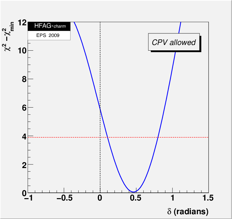
One-dimensional confidence curves for individual parameters are obtained by letting, for any value of the parameter, all other fitted parameters take their preferred values. The resulting functions Δ​χ2=χ2−χmin2\Delta\chi^{2}=\chi^{2}-\chi^{2}_{\rm min} are shown in Fig. 4. The points where Δ​χ2=3.84\Delta\chi^{2}=3.84 determine 95% C.L. intervals for the parameters, as shown in the figure. These intervals are listed in Table 3.

     Refer to caption    Refer to caption     Refer to caption    Refer to caption     Refer to caption    Refer to caption

Figure 4: The function Δ​χ2=χ2−χmin2\Delta\chi^{2}=\chi^{2}-\chi^{2}_{\rm min} for parameters x,y,δ,δK​π​π,|q/p|x,\,y,\,\delta,\,\delta_{K\pi\pi},\,|q/p|, and ϕ\phi. The points where Δ​χ2=3.84\Delta\chi^{2}=3.84 (denoted by the dashed horizontal line) determine a 95% C.L. interval.

4 Summary

We summarize the fit results listed in Table 3 and shown in Figs. 3 and 4 as follows:

  • •

    the experimental data consistently indicate that D0D^{0} mesons undergo mixing. The no-mixing point (x,y)=(0,0)(x,y)\!=\!(0,0) is excluded at 10.2​σ10.2\sigma. The parameter xx differs from zero by 3.2​σ3.2\sigma, and the parameter yy differs from zero by 4.8​σ4.8\sigma. The effect is presumably dominated by long-distance processes, which are difficult to calculate.

  • •

    Since yCPy_{\rm CP} is positive, the C​PCP-even state is shorter-lived, as in the K0K^{0}-K¯ 0\overline{K}{}^{\,0} system. However, since xx is also positive, the C​PCP-even state is heavier, unlike in the K0K^{0}-K¯ 0\overline{K}{}^{\,0} system.

  • •

    The strong phase difference δ\delta is probably not small: the fitted value is (26.4−9.9+9.6)∘(26.4\,^{+9.6}_{-9.9})^{\circ}.

  • •

    There is no evidence yet for C​P​VCPV in the D0D^{0}-D¯ 0\overline{D}{}^{\,0} system. Observing C​P​VCPV at the current level of sensitivity would indicate new physics.

5 Acknowledgments

We thank the organizers of the CHARM 2009 workshop for excellent hospitality and for a stimulating scientific program.

References

  • [1] See  http://www.slac.stanford.edu/xorg/hfag.
  • [2] The group has since expanded its activities to include calculating WA values of hadronic branching fractions, semileptonic form factors, properties of excited Ds∗⁣∗D^{**}_{s} states, and the Ds+D^{+}_{s} decay constant fDsf_{D_{s}}.
  • [3] I. Bigi and N. Uraltsev, Nucl. Phys. B592 (2001) 92.
  • [4] A. A. Petrov, “Charm Physics: Theoretical Review”, eConf C030603 (2003), arXiv:hep-ph/0311371; Nucl. Phys. Proc. Suppl. 142 (2005) 333.
  • [5] Charge-conjugate modes are implicitly included unless noted otherwise.
  • [6] E. M. Aitala et al. (E791 Collab.), Phys. Rev. Lett. 77 (1996) 2384; C. Cawlfield et al. (CLEO Collab.), Phys. Rev. D 71 (2005) 071101; B. Aubert et al. (Babar Collab.), Phys. Rev. D 76 (2007) 014018; U. Bitenc et al. (Belle Collab.), Phys. Rev. D 77 (2008) 112003.
  • [7] E. M. Aitala et al. (E791 Collab.), Phys. Rev. Lett. 83 (1999) 32; J. M. Link et al. (FOCUS Collab.), Phys. Lett. B485 (2000) 62; S. E. Csorna et al. (CLEO Collab.), Phys. Rev. D 65 (2002) 092001; K. Abe et al. (Belle Collab.), Phys. Rev. Lett. 88 (2002) 162001; M. Staric et al. (Belle Collab.), Phys. Rev. Lett. 98 (2007) 211803; B. Aubert et al. (Babar Collab.), Phys. Rev. D 78 (2008) 011105; A. Zupanc et al. (Belle Collab.), Phys. Rev. D 80 (2009) 052006; B. Aubert et al. (Babar Collab.), arXiv:0908.0761.
  • [8] http://www.slac.stanford.edu/xorg/hfag/charm/EPS09/
    results_mixing.html.
  • [9] D. M. Asner et al. (CLEO Collab.), Phys. Rev. D 72 (2005) 012001; arXiv:hep-ex/0503045 (revised April 2007); L. M. Zhang et al. (Belle Collab.), Phys. Rev. Lett. 99 (2007) 131803.
  • [10] L. M. Zhang et al. (Belle Collab.), Phys. Rev. Lett. 96 (2006) 151801; B. Aubert et al. (Babar Collab.), Phys. Rev. Lett. 98 (2007) 211802; T. Aaltonen et al. (CDF Collab.), Phys. Rev. Lett. 100 (2008) 121802.
  • [11] B. Aubert et al. (Babar Collab.), arXiv:0807.4544. See also: X. C. Tian et al. (Belle Collab.), Phys. Rev. Lett. 95 (2005) 231801.
  • [12] D. M. Asner et al. (CLEOc Collab.), Phys. Rev. D 78 (2008) 012001.