∎
Lyapunov Analysis for Fully Developed Homogeneous Isotropic Turbulence
Abstract
The present work studies the isotropic and homogeneous turbulence for incompressible fluids through a specific Lyapunov analysis, assuming that the turbulence is due to the bifurcations associated to the Navier-Stokes equations.
The analysis consists in the calculation of the velocity fluctuation through the Lyapunov analysis of the local deformation and the Navier-Stokes equations and in the study of the mechanism of the energy cascade from large to small scales through the finite scale Lyapunov analysis of the relative motion between two particles.
The analysis provides an explanation for the mechanism of the energy cascade, leads to the closure of the von Kármán-Howarth equation, and describes the statistics of the velocity difference.
Several tests and numerical results are presented.
Keywords:
Bifurcations Lyapunov Analysis von Kármán-Howarth equation Velocity difference statisticspacs
47.27.-i1 Introduction
In this work a novel procedure based on a specific Lyapunov analysis is presented
for studying the incompressible isotropic and homogeneous turbulence in an infinite domain.
The analysis is mainly motivated by the fact that in turbulence the kinematics
of the fluid deformation is subjected to bifurcations [1] and exhibits a chaotic behavior and huge mixing [2], [3], resulting to be much more rapid than the fluid
state variables.
This characteristics implies that the accepted kinematical hypotheses for deriving the Navier-Stokes equations could require the consideration of very small length scales and times for describing the fluid motion [4] and therefore a very large number of degrees of freedom.
As well known, other peculiar characteristics of the turbulence are the mechanism of the kinetic energy cascade, directly related to the relative motion of a pair of fluid particles [5], [6], [7], [8] and responsible for the shape of
the developed energy spectrum, and the non-gaussian statistics of the velocity difference.
This energy spectrum can be calculated through a proper closure of the von Kármán-Howarth equation (see Appendix) or of its Fourier Transform [7], [8]. The equation describes the evolution of the correlation function of the longitudinal velocity , and depends upon the term (see Appendix), directly related to the longitudinal triple-velocity correlation . This latter, due to the inertia forces, does not change the kinetic energy of the fluid and satisfies the detailed conservation of energy [8] which states that the exchange of energy between wave-numbers is only related to the amplitudes of these wave-numbers and of their difference [9].
Various authors (see for instance [10], [11], [12]), propose, for , the following diffusion approximation
| (1) |
where and are the separation distance and the turbulent diffusivity, whereas represents the longitudinal velocity standard deviation. This implies that the closed von Kármán-Howarth equation is a parabolic equation in any case (also for =0).
To the author knowledge, Hasselmann in 1958 [10] was the first that proposed a link between and , using a simple model which expresses in function of the momentum convected through the surface of a spherical volume. His model incorporates a free parameter and expresses by means of a complex expression.
Another closure model in the framework of Eq. (1) was developed by Millionshtchikov [11]. There, the author assumes that , where is an empirical constant. Although both the models describe two possible mechanisms of the energy cascade, in general, do not satisfy some physical conditions. For instance, the model of Hasselmann does not verify the continuity equation for all the initial conditions, whereas the Millionshtchikov’s model gives, according to Eq. (1), an absolute value of the skewness of , in contrast with the several experiments and with the energy cascade [8].
More recently, Oberlack and Peters [12] suggested a closure model where is in terms of , i.e. and is a constant parameter. The authors show that this closure reproduces the energy cascade and, for a proper choice of , provides results [12] in agreement with the experimental data of the literature.
In general, Eq. (1) represents models of diffusion approximation based on the assumption that the turbulence can be represented by an opportune diffusivity which varies with [8]. As a consequence of Eq. (1), contains a term proportional to which can occur only if the inertia forces include stochastic external terms, independent from the fluid state variables [13] and not present in the classical formulation [7], [8]. For this reason the models based on Eq. (1) are really phenomenological closure of Eq. (112).
Although several other works on the von Kármán-Howarth equation were written [14], [15], [16], [17], to the author’s knowledge, a theoretical analysis based on basic principles which provides a physical-mathematical closure of the von Kármán-Howarth equation and the statistics of has not received due attention. Therefore, the objective of the present work is to develop a theoretical analysis based on reasonable physical conjectures which allows the closure of the von Kármán-Howarth equation and the determination of the statistics of .
Of course, besides the von Kármán-Howarth equation, there are some other approaches, such as the direct numerical simulation based on solving the Navier-Stokes equations and the experiments, which are not considered in the present work.
The present work only considers the possibility to obtain the fully developed homogeneous-isotropic turbulence in a given condition and does not analyze the intermediate stages of the turbulence. The study assumes that the fluctuations of the fluid state variables are the result of the bifurcations of the Navier-Stokes equations. In section 2, we present a qualitative scenario of these bifurcations which leads to the onset of the turbulence. These bifurcations, defined by means of the fixed points of the velocity field and the Navier-Stokes equations, allows a rough estimation of the critical Reynolds number based on the Taylor scale. After, in section 3, the velocity fluctuation is studied through the kinematics of the local deformation and the momentum equations. These latter are expressed with respect to the referential coordinates which coincide with the material coordinates for a given fluid configuration [4], whereas the kinematics of the local deformation is analyzed with the Lyapunov theory. The choice of the referential coordinates allows the velocity fluctuations to be analytically expressed in terms of the Lyapunov exponent of the local fluid deformation. The section 4 deals with the study of the velocity difference between two fixed points of the space. This is analyzed with an opportune finite scale Lyapunov theory studying the motion of the particles crossing the two points, in the finite scale Lyapunov basis. This basis is formally obtained through the orthonormalization method of Gram-Schmidt of the finite scale Lyapunov vectors. These latter, also known as Bred vectors, were first introduced by Toth and Kalnay [18] to study the evolution in the time of a nonlinear perturbed model subjected to an initial finite perturbation. The choice of such vectors, whose properties are related to the classical Lyapunov vectors [19], is revealed to be an usefull tool for representing the relative motion of two particles crossing two given points of the space.
The present analysis postulates that the motion of such Lyapunov basis and that of the fluid with respect to the same basis, are completely statistically uncorrelated. This crucial assumption arises from the condition of fully developed turbulence. The study leads to the closure of the von Kármán-Howarth equation [7] and gives an explanation of the mechanism of the kinetic energy transfer between length scales.
The obtained expression of is the result of this assumption and does not correspond to a diffusive approximation with model free parameters. Its mathematical structure is in terms of and and satisfies the conservation law which states that the inertia forces only transfer the kinetic energy [7], [8]. This expression of corresponds to a first order term which makes the closed von Kármán-Howarth equation, a nonlinear partial differential equation of the first order in when . The main asset of the proposed closure on the other models is that it has been derived from a specific Lyapunov theory, with reasonable basic assumptions about the statistics of the velocity difference.
Furthermore, the statistics of the velocity difference is studied in section 7 with the Fourier analysis of the velocity fluctuations, and an analytical expression for the velocity difference and for its PDF is obtained in case of isotropic turbulence. This expression incorporates an unknown function, related to the skewness, which is identified through the obtained expression of . This velocity difference also requires the knowledge of the critical Reynolds number whose estimation is made in the section 2.
Finally, the several results obtained with this analysis are compared with the data existing in the literature, indicating that the proposed analysis adequately describes the various properties of the fully developed turbulence.
2 Bifurcations
This section qualitatively describes the route toward the turbulence by means of the bifurcations of the Navier-Stokes equations and provides an estimation of the critical Taylor scale Reynolds number, assuming that the turbulence is fully developed, homogeneous and isotropic.
The velocity field of a viscous and incompressible fluid, measured in the reference frame , satisfies the Navier-Stokes equations
Into Eq. (2), , , , , and , where and are assigned velocity and length, respectively. The pressure can be eliminated by taking the divergence of the momentum equation [8]. The velocity field, starting from the unique initial condition which does not depend on the Reynolds number, will depend upon by means of its time evolution
| (6) |
where represents the right-hand-side of the momentum Navier-Stokes equations calculated for .
Consider now the velocity field at , and the fixed points of Eq. (6) which, by definition, satisfy = 0 [20]. Increasing the Reynolds number, will vary according to Eq. (6), which can be expressed through the implicit function theorem [20]
| (7) |
where plays the role of the control parameter and is the fixed point calculated at , for . The location of these points will depend on the momentum Navier-Stokes equations and on the mathematical structure [20]. Therefore, influences the distribution of in the space.
According to the literature [21], [22], [23], [24] and to the characteristics of the diverse kinds of bifurcations, we assume the following qualitative scenario:
For small , the viscosity forces are stronger than the inertia ones and make an almost smooth function of . When the Reynolds number increases, as long as the Jacobian is nonsingular, exhibits smooth variations with , whereas at a certain , this Jacobian becomes singular ( = 0). This can correspond to the first bifurcation, where at least one of the eigenvalues of crosses the imaginary axis and appears to be discontinuous with respect to [20].
Figure 1 shows a scheme of bifurcations at , where the component of is reported in terms of . Starting from , the diagram is regular, until , where the first bifurcation determines two branches whose maximum distance is . and give, respectively, a length scale of the velocity field at the current value of , and the distance between two successive bifurcations. After , Eqs. (6) and (7) do not indicate which of the two branches the system will choose, thus a bifurcation causes a lost of informations with respect to the initial data [25]. That is, very small variations on the initial condition or very little perturbations, are of paramount importance for the choice of the branch that the system will follow [25]. This is the situation of the bifurcations at .

As the time increases, the position of the fixed points vary and so also the bifurcations, and far from the initial condition, one observes a developed motion, where the bifurcations can continuously vary with the time. Therefore, the bifurcations map changes with the time, and, if is high enough, the length scales are continuously distributed. In this case the energy spectrum can be continuous and, according to the theory [26], the velocity behaves as a chaotic function of and . There, the scales of Taylor and Kolmogorov are supposed to be assigned steady quantities.
To describe the road to turbulence, observe that the average distances depend on through Eqs. (6), and are here approximated by [20]
| (8) |
where , [21] and the average is calculated on the time. Equation (8) is supposed to describe the route toward the chaos and is assumed to be valid until the onset of the turbulence. There, the minimum for can not be less than the Kolmogorov scale [1], [26] where gives a good estimation of the correlation length of the phenomenon [20], [25] which, in this case is the Taylor scale . Thus, , and
| (9) |
where is the number of bifurcations at the beginning of the turbulence. Equation (9) gives the connection between the critical Reynolds number and . In fact, the characteristic Reynolds numbers associated to the scales and are 1 and , respectively, where is characteristic velocity at the Kolmogorov scale, and [8]. For isotropic turbulence, these scales are linked each other by [8]
| (10) |
In view of Eq. (9), this ratio can be also expressed through , i.e.
| (11) |
Assuming that is equal to the Feigenbaum constant (), the value 1.6 obtained for 2 is not compatible with which is the correlation scale, while the result 10.12, calculated for 3, is an acceptable minimum value for . The order of magnitude of these values can be considered in agreement with the various scenarios describing the roads to the turbulence [22], [21], [23], [24], and with the diverse experiments [27], [28], [29] which state that the turbulence begins for . Of course, this minimum value for is the result of the assumptions 2.502, , and of approximation (8).
3 Lyapunov analysis of the velocity fluctuations
In this section, the velocity fluctuations caused by the bifurcations of Eqs. (2) [1], are studied through the Lyapunov analysis of the kinematic of the fluid strain, using the Navier-Stokes equations.
Starting from the momentum Navier-Stokes equations written in a frame of reference
| (12) |
consider the map : , which is the function that determines the current position of a fluid particle located at the referential position [4] at . Equation (12) can be written in terms of the referential position [4]
| (13) |
where represents the stress tensor. The Lyapunov analysis of the fluid strain provides the expression of this deformation in terms of the maximal Lyapunov exponent
| (14) |
where is the maximal Lyapunov exponent and , are the Lyapunov exponents. Due to the incompressibility, 0, thus, .
The momentum equations written using the referential coordinates allow the factorization of the velocity fluctuation and to express it in Lyapunov exponential form of the local fluid deformation. If we assume that this deformation is much more rapid than and , the velocity fluctuation can be obtained from Eq. (13), where and are supposed to be constant with respect to the time
This assumption is justified by the fact that, according to Truesdell [4], is a smooth function of -at least during the period of a fluctuation- whereas the fluid deformation varies very rapidly in the vicinity of a bifurcation according to Eq. (14). This implies that, in proximity of bifurcations, the Lyapunov basis of orthonormal vectors [30] associated to the strain (14) rotates very quickly with respect to with an angular velocity , whereas the modulus of the fluid velocity fluctuation, measured in increases with a rate . Since is related to the maximal eigenvalue of , according to the fluid kinematics [2], [3], [31] . Therefore, the fluid velocity fluctuation measured in , varies very quickly because of the combined effect of the exponential growth rate and of the rotations of with respect to .
Note that, since is supposed to vary much more fastly than the fluid state variables, as long as does not exceed very much the Lyapunov time , the Lyapunov vectors almost coincide with the eigenvectors of and is nearly the maximum eigenvalue of [20].
4 Lyapunov analysis of the relative motion

In order to investigate the mechanism of the energy cascade, the relative motion between two fluid particles is here studied with the Lyapunov analysis.
Consider now two fixed points of the space, and (see Fig. 2) with , where is the separation distance, and the motion of the two fluid particles which at the time , cross through and . The equations of motion of these particles are
where and vary with the time according to the Navier-Stokes equations. is the relative position between the two particles, therefore .
The Lyapunov analysis of Eqs. (4) leads to the determination of the maximal finite scale Lyapunov exponent of Eqs. (2) and (4)
| (19) |
where , and represents the scale associated to . To define the finite scale Lyapunov basis of Eqs. (4), consider the system
The finite scale Lyapunov vectors , and are defined as the solutions of Eq. (4), starting from a given initial condition , ( =1, 2, 3) [18], where and vary according to Eqs. (4) and (2), respectively. Such vectors, also known as Bred vectors, are, by definition, related to the classical Lyapunov vectors in such a way that, , and tend to the classical Lyapunov vectors when , ( =1, 2, 3) [19], [32]. The finite scale Lyapunov basis of Eqs. (4) is then obtained by orthogonalizing , and with the Gram-Schmidt method at each time [30], [32].
This basis rotates with respect to with an angular velocity , where, because of isotropy . The fluid velocity difference , measured in , is expressed by the Lyapunov theory as
Into Eq. (4), is the Lyapunov exponent associated to the direction , where , and are, respectively, the components of and of and measured in . can be also written in terms of the maximal exponent
| (26) |
where , due to the other two exponents, is negligible with respect to and makes a solenoidal field, resulting during the fluctuation. When , maintains unchanged orientation with respect to . The velocity difference , measured in and expressed in , is calculated when
| (27) |
This equation states that determines the lateral components of the velocity difference in .
The longitudinal component of the velocity difference in , is then
| (28) |
where is the rotation matrix transformation from to , are the components of in , and is the unit vector along the longitudinal direction. Observe that, and arise both from the Navier-Stokes equations and that, in line with Eq. (19), can change but its variations are much slower than [20]. Moreover, the Lyapunov vectors sweep a subdomain of their space of state which coincides with the physical space . The simultaneous variations of these quantities produce the velocity difference fluctuation observed in , according to Eq. (28).
Although and arise from Eqs. (4) and (4), these are not directly related, therefore, we suppose here that is statistically orthogonal to both and , with . This is the crucial assumption of the present work which is justified by the condition of fully developed turbulence. This provides that
| (29) |
where the angular brackets denote the average calculated on the statistical ensemble of all the pairs of particles which cross through and . Again thanks to the fully developed turbulence, we also suppose that and are statistically orthogonal each other. This implies that
| (30) |
whereas the isotropy gives
| (31) |
where , and , (), are expressed in , and
| (32) |
Because of homogeneity, do not depend on .
Under these hypotheses, we now show the following equations
| (33) |
| (34) |
where , and are the components of along and along the two orthogonal directions and , and is a proper constant of the order of unity. The function is the lateral velocity correlation function (see Appendix) measured in , that due to the homogeneity and isotropy, coincides with the lateral correlation function measured in .
To demonstrate Eq. (34), observe that and can be decomposed into independent, identically distributed, stochastic variables , which satisfy [33]
| (35) |
where if , else and . is expressed as the sum of , where, without loss of generality, the coefficients of the combination are assumed constant with respect to and equal each other [33].
| (36) |
with constant parameters. The component (and ) is also expressed as the linear combination of , whose coefficients are now functions of as the consequence of the previous assumption, i.e.
| (37) |
Hence, the correlation function is in terms of and is determined through Eq. (37) and (35) [33], putting .
| (38) |
Therefore, is calculated taking into account Eq. (36), (37), (38) and (35), and, as a result, Eq. (34) is achieved.
5 Closure of the von Kármán-Howarth equation
Now, we present the closure of the von Kármán-Howarth equation based on the analysis seen at the previous section.
The term representing the inertia forces in the von Kármán-Howarth equation satisfies the identity (113) (see Appendix), which is here written as [7], [8]
| (39) |
where, due to the isotropy is a function of alone [7]. The divergence of gives the mechanism of the energy cascade which does not depend upon the frame of reference [7] [8]. In order to determine the expression of , Eq. (39) is here written in . In view of Eq. (27) and taking into account that is also frame independent, one obtains the following equation
| (40) |
Since is calculated with Eq. (19), this is constant with respect to the statistics of and , thus , and is expressed as the general integral of Eq. (40)
| (41) |
Into Eq. (41), is the sum of a term due to plus an arbitrary solenoidal field arising from the integration of Eq. (40) [34]. According to this analysis of Lyapunov, is proportional to and can be written in the form
| (42) |
Substituting Eq. (109) (see Appendix) and Eq. (42) into Eq. (41), is
| (43) |
where is the longitudinal velocity correlation function.
Equation (43) is made by three addends. In the first one of these, the part into the brackets is an even function of which goes to zero as and assumes the value for . The second term, orthogonal to the first one, vanishes at and tends to zero when . In this latter is expressed in for sake of convenience
| (44) |
The first term at the RHS of Eq. (44) vanishes because of Eq. (33), whereas the other ones are expressed by means of Eq. (34). Therefore
| (45) |
where and are from Eq. (34).
In order to satisfy Eq. (43), the expression of must be of the kind , where, because of homogeneity and according to Refs. [8] and [35], and are even functions of . Moreover, due to the isotropy and without lack of generality, [8], [35], so is
| (46) |
where , .
To determine and , Eq. (41) is projected along the directions and
From Eq. (5)
| (51) |
where . As , maintains unchanged orientation in , thus is an invariant which has to be identified. The function is determined with Eq. (5)
satisfies the conditions and [8], which represent, respectively, the homogeneity of the flow and the condition that the inertia forces do not modify the fluid kinetic energy. Since , this immediately identifies and
Due to the fluid incompressibility, and are related each other through (see Eq. (111), Appendix), leading to the expression
| (56) |
This expression of has been obtained studying the properties of the velocity difference in .
Equation (56) states that, the fluid incompressibility, expressed by , represents a sufficient condition to state that 0. This latter is determined as soon as is known. To calculate , it is convenient to express in , with . Thus, is first expressed in terms of and through Eq. (28) (), then its standard deviation is calculated assuming that , (i.e. ) and taking into account that and satisfy Eq. (31), with = 0:
where
and
represents the Levi-Civita tensor arising from
the cross product.
Since is the average of the velocity increment per unit distance, it is constant with respect the statistics of and , thus
.
Because of Eq. (30), and are
statistically independent, so that
0 and
,
therefore second and third terms vanish into Eq. (5).
Due to the isotropy, the Lyapunov basis satisfies Eq. (31)
(). This
is introduced in the first term of Eq. (5), which thus depends on alone.
This term, which equals , is associated to the direction
(maximal Lyapunov exponent direction) and represents one degree of freedom in the space.
Again thanks to the isotropy, the last term of Eq. (5) is two times the first one because it is caused by which corresponds to the two directions
orthogonal to and thus to two degrees of freedom.
As a result, taking into account that
,
the standard deviation of the longitudinal velocity difference is
| (61) |
with
| (62) |
This standard deviation can be expressed through the longitudinal correlation function
| (63) |
being the standard deviation of the longitudinal velocity. The maximal Lyapunov exponent is calculated in function of , from Eqs. (61) and (63)
| (64) |
Hence, substituting Eq. (64) into Eq. (56), one obtains the expression of in terms of and its gradient
| (65) |
This is the proposed closure of the von Kármán-Howarth equation, the main asset of which on the different diffusion models is that it has been derived from a specific Lyapunov analysis, under the assumption of reasonable statistical hypotheses about the longitudinal velocity difference. According to Eq. (65), is a nonlinear term of the first order, thus it does not represent a diffusion approximation, but rather a nonlinear advection term which makes Eq. (112) a nonlinear partial differential equation of the first order when .
Equation (65) corresponds to a mechanism of the kinetic energy transfer which preserves the average values of the momentum and of the kinetic energy. Specifically, the analytical structure of Eq.(65) states that this mechanism consists of a flow of the kinetic energy from large to small scales which only redistributes the kinetic energy between wavelengths.
This mechanism can be interpreted as follows. If, at , a toroidal volume is taken which contains and (see Fig. 2), its geometry and position change according to the fluid motion, and its dimensions, and , vary with the time to preserve the volume. Choosing in such a way that increases with the time, the Lyapunov analysis of Eqs. (4) leads to . According to the theory [20], for , the trajectories of the two particles are enclosed into . Hence, the kinetic energy, initially enclosed into , at the end of the fluctuation is contained into whose dimensions are changed with respect to . The kinetic energy is then transferred far from and , resulting enclosed in a more thin toroid.
6 Skewness of the velocity difference PDF
The obtained expression of allows to determine the skewness of [8]
| (66) |
which is expressed in terms of the longitudinal triple correlation , linked to by (also see Appendix, Eq. (114)). Since and are, respectively, even and odd functions of with = 1, =0, is given by
| (67) |
where the apex denote the derivative with respect to . To obtain , observe that, near the origin, behaves as
then, substituting Eq. (6) into and accounting for Eq. (67), one obtains
| (70) |
is a constant of the present analysis, which does not depend on the Reynolds number. This is in agreement with the several sources of data existing in the literature such as [8], [36], [37], [38] (and Refs. therein) and its value gives the entity of the mechanism of the energy cascade.
This skewness causes variations in the time of the Taylor scale in accordance to Eq. (112). The time derivative of is calculated considering the coefficients of the order in the von Kármán-Howarth equation [7], [8] which are determined substituting Eqs. (6) and (70) into Eq. (112)
| (71) |
where . The first term tends to decrease and expresses the mechanism of energy cascade, whereas the term in the brackets gives the viscosity effect which, in general, tends to increase depending on the current values of and [7], [8].
7 Statistical analysis of the velocity difference
As explained in this section, the Lyapunov analysis of the local deformation and some plausible assumptions about the statistics of the velocity difference lead to determine all the statistical moments of with only the knowledge of the function and of the value of the critical Reynolds number.
The statistical properties of , are investigated expressing the velocity fluctuation, given by Eq. (3), as the Fourier series
| (72) |
where are the components of the velocity spectrum, which satisfy the Fourier transformed Navier-Stokes equations [8]
All the components are random variables distributed according to certain distribution functions, which are statistically orthogonal each other [8].
Thanks to the local isotropy, is sum of several dependent random variables which are identically distributed [8], therefore tends to a gaussian variable [33], and satisfies the Lindeberg condition, a very general necessary and sufficient condition for satisfying the central limit theorem [33]. This condition does not apply to the Fourier coefficients of . In fact, since is the difference between two dependent gaussian variables, its PDF could be a non gaussian distribution function. In , the velocity difference is given by
| (75) |
This fluctuation consists of the contributions appearing into Eq. (7): in particular, represents the sum of all linear terms due to the viscosity and is the sum of all bilinear terms arising from inertia and pressure forces. and are, respectively, the sums of definite positive and negative square terms, which derive from inertia and pressure forces. The quantity tends to a gaussian random variable being the sum of statistically orthogonal terms [39], [33], while and do not, as they are linear combinations of squares [39]. Their general expressions are [39]
where and are constants, and , , and are four different centered random gaussian variables. Therefore, the fluctuation of the longitudinal velocity difference can be written as
where , and are independent centered random variables which have gaussian distribution functions with standard deviation equal to the unity. The parameter is a positive definite function of the Reynolds number, whereas and are functions of the space coordinates and the Reynolds number.
At the Kolmogorov scale , the order of magnitude of the velocity fluctuations is , with and , whereas is negligible because is due to the inertia forces: this immediately identifies .
On the contrary, at the Taylor scale , is negligible and the order of magnitude of the velocity fluctuations is , therefore .
The ratio is a function of
| (82) |
where , is a function which has to be determined.
Hence, the dimensionless longitudinal velocity difference , is written as
The dimensionless statistical moments of are easily calculated considering that , and are independent gaussian variables
where
In particular, the third moment or skewness, , which is responsible for the energy cascade, is
| (97) |
For 1, the skewness and all the odd order moments are different from zero, and for , all the absolute moments are rising functions of , thus exhibits an intermittency whose entity increases with the Reynolds number.
All the statistical moments can be calculated once the function and the value of are known. The expression of obtained in the first part of the work allows to identify and then fixes the relationship between and
| (98) |
where and . This relationship does not admit solutions with below a minimum value of dependent on . According to the analysis of section 2, is chosen to 10.12, which corresponds to . (setting , = 10.12 in ). Varying the value of from 8.5 to 15 would bring values of between 1.2 and 0.9, respectively. In figure 3, the function is shown for . The limit 0.86592 for is reached independently of the value of .

The PDF of is expressed through the Frobenius-Perron equation
where is calculated with Eq. (7), is the Dirac delta and is a gaussian PDF whose average value and standard deviation are equal to 0 and 1, respectively.
For non-isotropic turbulence or in more complex cases with boundary conditions, the velocity spectrum could not satisfy the Lindeberg condition, thus the velocity will be not distrubuted following a Gaussian PDF, and Eq. (7) changes its analytical form and can incorporate more intermittant terms [33] which give the deviation with respect to the isotropic turbulence. Hence, the absolute statistical moments of will be greater than those calculated with Eq. (7), indicating that, in a more complex situation than the isotropic turbulence, the intermittency of can be significantly stronger.
8 Results and discussion
In order to validate the results of the proposed Lyapunov analysis, several data are now presented.
As the first result, the evolution in the time of is calculated with the proposed closure (Eq. (65)) of the von Kármán-Howarth equation, where the boundary conditions are given by Eq. (115) (see Appendix). The turbulent kinetic energy and and are calculated with Eq. (116) and Eqs. (10), respectively. The calculation is carried out for an initial Reynolds number of = 2000, where and are, respectively, the reference dimension and the initial velocity standard deviation. The initial condition for is , where = , whereas = 1. The dimensionless time of the problem is defined as .

Equation (112) was numerically solved adopting the Crank-Nicholson integrator scheme with variable time step , whereas the discretization in the spatial domain is made by intervals of the same amplitude . The truncation error of the scheme of integration is , where is automatically selected by the algorithm in such a way that for each time step, thus the accuracy of the scheme is of the order of . As the consequence, the discretization of the Fourier space is made by subsets in the interval , where = . For the adopted initial Reynolds number the choice = 1500 gives an adequate discretization, which provides , for the whole simulation. For what concerns , it was calculated with Eq. (116) and the kinetic energy was checked to be equal to the integral over of . During the simulation, must identically satisfy Eq.(124) (see Appendix) which states that does not modify the kinetic energy. The integral of is calculated with the trapezoidal formula, for , and the simulation will be considered to be accurate as long as
| (101) |
namely, when for . As the simulation advances, according to Eq. (65), the energy cascade determines variations of and for values of which rise with the time and that can occur out of the interval (, ). Thus, Eq. (101) holds until a certain time, where these wave-numbers are about equal to . For higher times, the variations of occur for , out of the interval of numerical integration , and Eq. (101) could not be satisfied. Hence, the results of the simulation will be accurate until reaching of the following condition [40]
| (102) |
where the right-hand side represents the estimation of the truncation error of the trapezoid formula [40]. There, it is found that, in all the simulations. . Thereafter, the numerical method loses its consistency, since the violation of Eq. (101) implies that does not preserve the kinetic energy. Nevertheless, the error committed by the algorithm is considered still acceptable as long as [7], [8]
| (103) |
That is to say, when the numerical residual of the rate of energy transfer is much less than the dissipation rate. In any case the simulations are stopped if reaches its relative minimum in function of the time with , or as soon as . The accuracy of the solutions is evaluated through the check of Eq. (103). At end of simulation, we assume that the energy spectrum is fully developed.
In order to study the proposed closure, we first analyze the case with . In this case, with the assumed initial condition, Eq. (112) admits the analytical self-similar solution [7]
| (104) |
maintains its shape unchanged in function of the dimensionless coordinate . The corresponding numerical solutions were calculated for different spatial discretization (i.e. = , , and ). All these simulations satisfy Eq. (104), with a calculated error which is always of the order of the truncation error of the scheme of integration. Also the energy spectrum preserves its shape, and is given by , with , [8].
Consider now the case, where is given by Eq. (65). The diagrams of Fig. 4 show the evolution of and in terms of , at different times of simulation. The kinetic energy and vary according to Eqs. (65), (116) and (71), thus and change in such a way that their scales, in particular and , diminish as the time increases, whereas the maximum of decreases. That is, Eq. (65) corresponds to a transferring of the energy toward the smaller scales which strongly contrasts the effects of viscosity seen in the previous case.
At the final instants of the simulation, one obtains that O( ) for O(1), and the maximum of is about 0.05. These results are in very good agreement with the numerous data of the literature [8] which concern the evolution of in homogeneous isotropic turbulence.

Figure 5 shows the diagrams of and , at the same times, in comparison with the Kolmogorov law () and with the incompressibility condition (). The energy spectrum depends on the initial condition, and at the end of the simulation, can be compared with the Kolmogorov spectrum in an opportune interval of wave-numbers which defines the inertial subrange. This arises from , which, at the final times, behaves like = O () for . satisfies the continuity equation which implies that near the origin.

In the figure, the dimensionless time corresponds to the condition (102), whereas (bold dashdotted line) represents the spectrum calculated when reaches its minimum in function of the time. In this last situation, the algorithm is less accurate, due to the discretization. In fact, , (bold dashdotted), exhibits small nonzero values in a wide range of variations of , for . Although Eq. (101) is not satisfied, the error of the algorithm is still acceptable since the absolute value of the integral of over () is about four orders of magnitude less than the dissipation rate (see Eq. (103)).

To study the effect of the spatial discretization on the final energy spectrum, Fig. 6 shows the results of other simulations which were performed for = 500, 1000. It is found that, for = 500 and 1000, the stopping criterion is satisfied for , whereas the final times of simulation rises with , resulting that and for = 500 and 1000, respectively. As the consequence, also the inertial subrange of Kolmogorov increase with .
In order to compare the results of the present analysis with the data in the literature, a further calculation has been carried out with an initial Reynolds number of . The present results (continuous line) are shown in Fig. 7, in terms of energy spectrum, and are compared with those calculated, for the same conditions, with the Oberlack’s model [12] (dashed line). For this latter, the parameter [12] (see introduction) is assumed to be equal to . For this value of , the Oberlack’s model gives the same value of skewness , calculated with the present analysis. Thus, the entity of the mechanism of the energy cascade is the same in both the cases. Again, the initial correlation function is , and 1500.
Equation (101) is satisfied until a certain time (i.e. for Oberlack’s model and for the present analysis), therafter the numerical scheme exhibits a minor accuracy, since for ). In the figure, the energy spectrum is shown at the end of the two simulations which happen at (Oberlack) and at (Present Analysis), where the stopping condition is satisfied for min . There, the integral of is, in both the cases, much less than (about four orders of magnitude) and for this reason the results of the two simulations can be considered accurate enough. Since the skewness is the same in the two cases, the variations of almost coincide during the simulations, a part very small variations caused by (see Eq. (71)) which are not appreciated in the figure. Therefore, also is about the same in both the cases. Nevertheless, the energy spectra show significative differences. The spectrum calculated with Eq. (65) exhibits a wider range of wave-numbers than the other one, and this is due to the fact that Eq. (65) represents a nonlinear term of the first order which does not cause any diffusion effect, whereas for the Oberlack’s model, the closure term is of the second order and the variable eddy diffusivity produces a sizable reduction of all the wave-numbers, especially for large . The wave-number calculated where (see figure), is quite different in the two cases. Specifically, the present analysis gives a value two times greater than in the Oberlack’s model, and, as the consequence, also the Kolmogorov inertial subrange calculated with the present analysis is about two times the other one.
Next, the Kolmogorov function and Kolmogorov constant , are determined, using the results of the previous simulations.
Following the Kolmogorov theory, the Kolmogorov function, which is defined as
| (105) |
is constant w. r. t. , and is equal to 4/5 as long as . As shown in Fig. 8, for , is significantly greater than and the variations of with can not be neglected. This is the consequence of the choice of the initial correlation function. At the successive times, decreases until the final instants, where, with the exception of , exhibits variations which are less than those calculated at the previous times in a wide range of , with a maximum which can be compared to 0.8.

The Kolmogorov constant is also calculated by
| (106) |
For and 0.63, and , whereas for 0.69, , . For at end simulation (i.e. 0.67), , , namely and agree with the corresponding quantities known from the literature.
For , Fig. 9a shows the maximal finite scale Lyapunov exponent, calculated with Eq. (64). For , the variations of are the result of the adopted initial correlation function which is a gaussian, whereas as increases, the variations of determine sizable increments of and of its slope in proximity of the origin. Then, for , since , the maximal finite scale Lyapunov exponent behaves like . Thus, the Richardson’s diffusivity associated to the relative motion between two fluid particles, defined as [5], here satisfies the famous Richardson scaling law [5] in proximity of the end of the simulation.
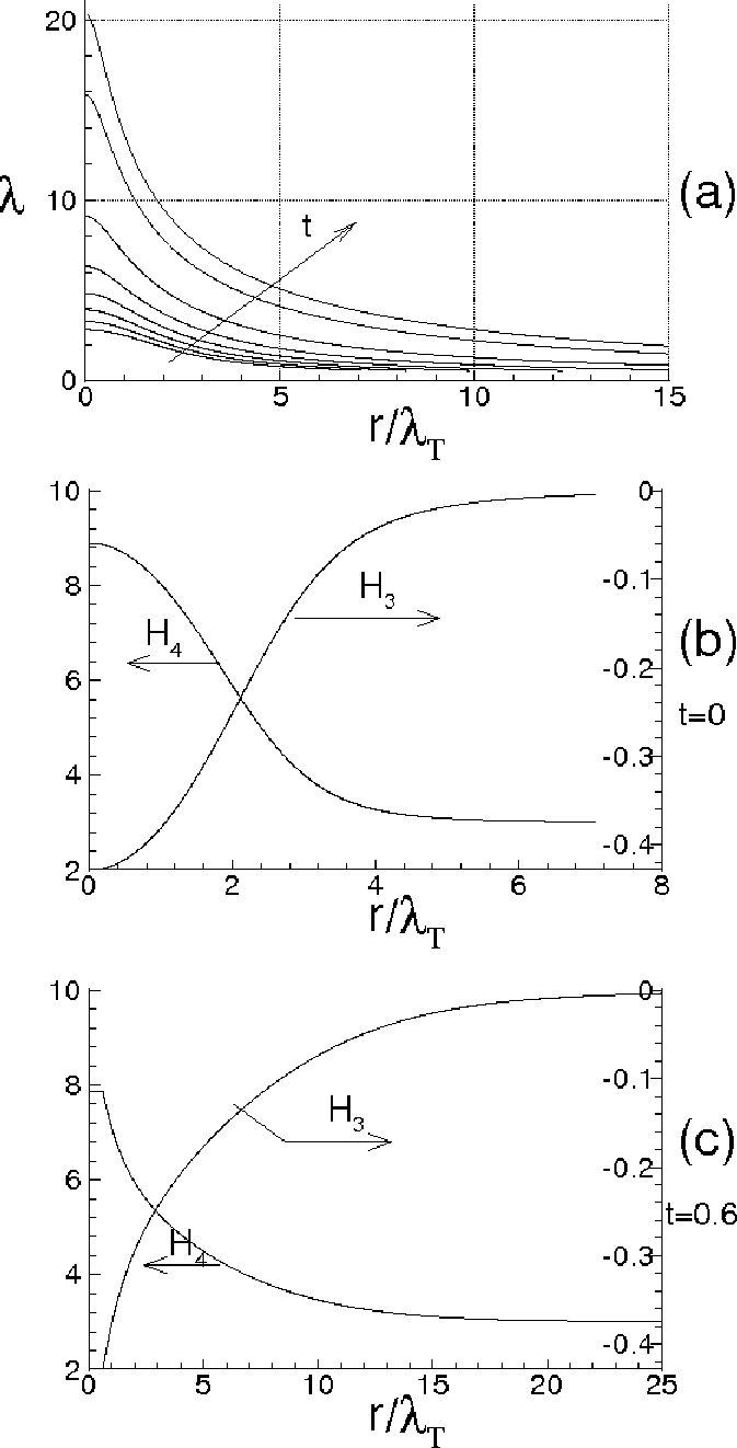

In the figures 9b and 9c, skewness and flatness of are shown in terms of for = 0 and 0.6 and . The skewness, is first calculated with Eq. (66), then has been determined using Eq. (7). At , starts from 3/7 at the origin with small slope, then decreases until reaching small values. also exhibits small derivatives near the origin, where 3, thereafter it decreases more rapidly than . At 0.6, the diagram importantly changes and exhibits different shapes. The Taylor scale and are both changed, so that the variations of and are associated to smaller distances, whereas the flatness at the origin is slightly less than that at . Nevertheless, these variations correspond to higher values of than those for = 0, and again reaches the value of 3 more rapidly than tends to zero.
The PDFs of are calculated, for , with Eqs. (7) and (7), and are shown in Fig. 10 in terms of the dimensionless abscissa
where, these distribution functions are normalized, in order that their standard deviations are equal to the unity. The figure represents the distribution functions of for several , at = 0, 0.5 and 0.6, where the dotted curves represent the gaussian distribution functions. The calculation of is first carried out with Eq. (66), then is identified through Eq. (97), and finally the PDF is obtained with Eq. (7). For = 0 (see Fig. 10a) and according to the evolutions of and , the PDFs calculated at 0 and 1, are quite similar each other, whereas for 5, the PDF is almost a gaussian function. Toward the end of the simulation, (see Fig. 10b and c), the two PDFs calculated at 0 and 1, exhibit more sizable differences, whereas for 5, the PDF differs very much from a gaussian PDF. This is in line with the plots of and of Fig. 9.

Next, the spatial structure of , given by Eq. (7), is analyzed using the previous results. According to the various works [41], [42], behaves quite similarly to a multifractal system, where obeys to a law of the kind where the exponent is a fluctuating function of the space coordinates. This implies that the statistical moments of are expressed through different scaling exponents whose values depend on the moment order , i.e.
| (107) |
| Re(0) | P | 1 | 2 | 3 | 4 | 5 | 6 | 7 | 8 | 9 | 10 | 11 | 12 | 13 | 14 |
|---|---|---|---|---|---|---|---|---|---|---|---|---|---|---|---|
| 2000 | (P) | 0.36 | 0.71 | 1.00 | 1.19 | 1.41 | 1.61 | 1.84 | 2.04 | 2.25 | 2.49 | 2.72 | 2.93 | 3.15 | 3.38 |
| 3000 | (P) | 0.36 | 0.72 | 1.00 | 1.19 | 1.43 | 1.64 | 1.84 | 2.03 | 2.25 | 2.49 | 2.71 | 2.92 | 3.11 | 3.33 |
These scaling exponents are here identified through a best fitting procedure, in the interval ( ), where the endpoints is an unknown quantity which has to be determined. The location of this interval varies with the time. The calculation of , and is carried out through a minimum square method which, for each moment order, is applied to the following optimization problem
| (108) |
where are calculated with Eqs. (7), and is calculated
in order to obtain .
Figure 11 shows the comparison between the scaling exponents here obtained (continuous lines with solid symbols) and those of the Kolmogorov theories K41 [6] (dashed lines) and K62 [41] (dashdotted lines), and those given by She-Leveque [42] (dotted curves).
At 0, the values of are the result of the chosen initial condition.
As the time increases, changes causing variations in the statistical
moments of . As result, gradually diminish and exhibit a variable slope which depends on the moment order , until to reach the situation of
Fig. 11b, where the simulation is just ended.
The dimensionless moments of are changed. The plot of shows that near the origin, , and that the values of seem to be in agreement with the those proposed by She-Leveque.
More in detail, Table I reports these scaling exponents in terms of the moments order, calculated for .
These values and the peculiar diagram of Fig. (11) are the consequence of the spatial variations of the skewness, calculated using Eq. (66), and of the quadratic terms due to the inertia and pressure forces into the expression of the velocity difference, which make
a quantity quite similar to a multifractal system.
Other simulations with different initial correlation functions and Reynolds numbers have been carried out, and all of them lead to analogous results, in the sense that, at the end of the simulations, the diverse quantities such as , and are quite similar to those just calculated. For what concerns the effect of the Reynolds number, its increment determines a wider range of the wave-numbers where is comparable with the Kolmogorov law and a smaller dissipation energy rate in accordance to Eq. (116).
| Moment | Gaussian | |||
|---|---|---|---|---|
| Order | P. R. | P. R. | P. R. | Moment |
| 3 | -.428571 | -.428571 | -.428571 | 0 |
| 4 | 3.96973 | 7.69530 | 8.95525 | 3 |
| 5 | -7.21043 | -11.7922 | -12.7656 | 0 |
| 6 | 42.4092 | 173.992 | 228.486 | 15 |
| 7 | -170.850 | -551.972 | -667.237 | 0 |
| 8 | 1035.22 | 7968.33 | 11648.2 | 105 |
| 9 | -6329.64 | -41477.9 | -56151.4 | 0 |
| 10 | 45632.5 | 617583. | 997938. | 945 |
In order to study the evolution of the intermittency vs. the Reynolds number, Table II gives the first ten statistical moments of . These are calculated with Eqs. (7) and (7), for = 10.12, 100 and 1000, and are shown in comparison with those of a gaussian distribution function. It is apparent that a constant nonzero skewness of , causes an intermittency which rises with (see Eq. (7)). More specifically, Fig. 12 shows the variations of and (continuous lines) in terms of , calculated with Eqs. (7) and (7), with . These moments are rising functions of for 10 700, whereas for higher these tend to the saturation and such behavior also happens for the other absolute moments. According to Eq. (7), in the interval 10 70, and result to be about proportional to and , respectively, and the intermittency increases with the Reynolds number until 700, where it ceases to rise so quickly.


This behavior, represented by the continuous lines, depends on the fact that , and results to be in very good agreement with the data of Pullin and Saffman [43], for 10 100.


Figure 12 can be compared with the data collected by Sreenivasan and Antonia [38], which are here reported into Fig. 13. These latter are referred to several measurements and simulations obtained in different situations which can be very far from the isotropy and homogeneity conditions. Nevertheless a comparison between the present results and those of Ref. [38] is an opportunity to state if the two data exhibit elements in common. According to Ref. [38], the flatness monotonically rises with with a rising rate which agrees with Eq. (7) for (dashed line, Fig. 12), whereas the skewness seems to exhibit minor variations. Thereafter, continues to rise with about the same rate, without the saturation observed in Fig. 12. The weaker intermittency calculated with the present analysis seems arise from the isotropy which makes a gaussian random variable, while, as seen in sec. 6, without the isotropy, the flatness of and can be much greater than that of the isotropic case.
Next, the obtained results are compared with the data of Tabeling et al [36], [37]. There, in an experiment using low temperature helium gas between two counter-rotating cylinders (closed cell), the authors measure the PDF of and its moments. Again, the flow could be quite far from to the isotropy condition, since these experiments pertain wall-bounded flows, where the walls could importantly influence the fluid velocity in proximity of the probe. The authors found that moments , with , first increase with until 700, then exhibit a lightly non-monotonic evolution with respect to , and finally cease their variations, denoting a transition behavior (See Fig. 14). As far as the skewness is concerned, the authors observe small percentage variations. Although the isotropy does not describe the non-monotonic evolution near 700, the results obtained with Eq. (7) can be considered comparable with those of Refs. [36], [37], resulting again, that the proposed analysis gives a weaker intermittency with respect to Refs. [36], [37].
The normalized PDFs of are calculated with Eqs. (7) and (7), and are shown in Fig. 15 in terms of the variable , which is defined as
Figure 15a shows the diagrams for 15, 30 and 60, where
the PDFs vary in such a way that .
As well as in Ref. [37], Figs. 4b and 4c give the PDF for
= 255, 416, 514, 1035 and 1553, where these last Reynolds numbers are calculated through the Kolmogorov function given in Ref. [37], with .
In particular, Fig. 15c represents the enlarged region of Fig. 15b, where the tails of PDF are shown for .
According to Eq. (7), the tails of the PDF rise in the interval
10 700,
whereas at higher values of , smaller variations occur.
Although the trend observed in Fig. 16 [37] is non-monotonic,
Fig. 15c shows that the values of the PDFs
calculated with the proposed analysis, for , exhibit the same
order of magnitude of those obtained by Tabeling et al
[37].

Asymmetry and intermittency of the distribution functions are also represented through the integrand function of the order moment of PDF, which is . This function is shown in terms of , in Fig. 17, for = 15, 30 and 60.
9 Conclusions
The proposed analysis is based on the conjecture that the turbulence is caused by the bifurcations and that the kinematic of the relative motion is much more rapid than the fluid state variables. The analysis also assumes statistical hypotheses about the velocity difference, which derive from the condition of fully developed turbulence. The main limitation of this analysis is that it only studies the developed homogeneous-isotropic turbulence, whereas this does not consider the intermediate stages of the turbulence.
The results can be here summarized:
- 1.
The qualitative analysis of the bifurcations leads to determine the order of magnitude of the critical Reynolds number based on the Taylor scale and the number of the bifurcations at the onset of the turbulence.
- 2.
The momentum equations written using the referential coordinates allow to factorize the velocity fluctuation and to express it in Lyapunov exponential form of the local fluid deformation. As a result, the velocity fluctuation is the combined effect of the exponential growth rate and of the rotations of the Lyapunov basis with respect to the fixed frame of reference.
- 3.
The finite scale Lyapunov analysis of the relative motion provides an explanation of the physical mechanism of the energy cascade in turbulence and gives a closure of the von Kármán-Howarth equation. This is a non-diffusive closure which depends on the local values of the longitudinal correlation function and on its spatial gradient.
The fluid incompressibility is a sufficient condition to state that the inertia forces transfer the kinetic energy between the length scales without changing the total kinetic energy. This implies that the skewness of the longitudinal velocity derivative is a constant of the present analysis and that the energy cascade mechanism does not depend on the Reynolds number.
- 4.
The statistics of can be inferred looking at the Fourier series of the velocity difference. This is a non-Gaussian statistics, where the constant skewness of implies that the other higher absolute moments increase with the Taylor-scale Reynolds number.
- 5.
The proposed closure of the von Kármán-Howarth equation, shows that the mechanism of energy cascade gives energy spectrum that can be compared with the Kolmogorov law in an opportune range of wave-numbers and which satisfy the incompressibility condition.
- 6.
For developed energy spectrum, the Kolmogorov function exhibits, in an opportune range of , small variations much less than at the previous times, and its maximum is quite close to 4/5, whereas the Kolmogorov constant is about equal to 1.93. As the consequence, the maximal finite scale Lyapunov exponent and the diffusivity coefficient vary according to the Richardson law when the separation distance is of the order of the Taylor scale.
- 7.
The analysis also determines the scaling exponents of the moments of the longitudinal velocity difference through a best fitting procedure. For developed energy spectrum, these exponents show variations with the moment order consistent with those present in the literature.
10 Appendix
The von Kármán-Howarth equation gives the evolution in the time of the longitudinal correlation function for isotropic turbulence. The correlation function of the velocity components is the symmetrical second order tensor , where and are the velocity components at and , respectively, being the separation vector. The equations for are obtained by the Navier-Stokes equations written in the two points and [7], [8]. For isotropic turbulence can be expressed as
| (109) |
and are, respectively, longitudinal and lateral correlation functions, which are
| (110) |
where and are, respectively, the velocity components parallel and normal to , whereas and = == . Due to the continuity equation, and are linked each other by the relationship
| (111) |
The von Kármán-Howarth equation reads as follows [7], [8]
| (112) |
where is an even function of , defined as [7], [8]
| (113) |
and which can also be expressed in terms of the longitudinal triple correlation function
| (114) |
The boundary conditions of Eq. (112) are [7], [8]
| (115) |
The viscosity is responsible for the decay of the turbulent kinetic energy, the rate of which is [7], [8]
| (116) |
This energy is distributed at different wave-lengths according to the energy spectrum which is calculated as the Fourier Transform of , whereas the ”transfer function” is the Fourier Transform of [8], i.e.
where and identically satisfies to the integral condition
| (124) |
which states that does not modify the total kinetic energy. The rate of energy dissipation is calculated for isotropic turbulence as follows [8]
| (125) |
The microscales of Taylor , and of Kolmogorov , are defined as
References
- (1) Landau, L. D., Lifshitz, M, Fluid Mechanics. Pergamon London, England, 1959.
- (2) Ottino, J. M. The kinematics of mixing: stretching, chaos, and transport, Cambridge Texts in Applied Mathematics, New York, 1989.
- (3) Ottino, J. M., Mixing, Chaotic Advection, and Turbulence., Annu. Rev. Fluid Mech. 22, 207–253, 1990.
- (4) Truesdell, C. A First Course in Rational Continuum Mechanics, Academic, New York, 1977.
- (5) Richardson, L. F, Atmospheric Diffusion shown on a distance–neighbour graph., Proc. Roy. Soc. London, A 110, 709, 1926.
- (6) Kolmogorov, A. N., Dissipation of Energy in Locally Isotropic Turbulence. Dokl. Akad. Nauk SSSR 32, 1, 19–21, 1941.
- (7) von Kármán, T., Howarth, L., On the Statistical Theory of Isotropic Turbulence., Proc. Roy. Soc. A, 164, 14, 192, 1938.
- (8) Batchelor, G.K., The Theory of Homogeneous Turbulence. Cambridge University Press, Cambridge, 1953.
- (9) Eyink G. L. & Sreenivasan K.R. , Onsager and the theory of hydrodynamic turbulence, Rev. Mod. Phys., 78, 87–-135, 2006.
- (10) Hasselmann K., Zur Deutung der dreifachen Geschwindigkeitskorrelationen der isotropen Turbulenz, Dtsch. Hydrogr. Z, 11, 5, 207-217, 1958.
- (11) Millionshtchikov M., Isotropic turbulence in the field of turbulent viscosity, JETP Lett., 8, 406–411, 1969.
- (12) Oberlack M., Peters N., Closure of the two-point correlation equation as a basis for Reynolds stress models, Appl. Sci. Res., 51, 533–539, 1993.
- (13) Skorokhod A. V. Stochastic equations for complex systems, Springer-Verlag, Berlin, Heidelberg, New York, 1988.
- (14) Domaradzki J. A., Mellor G. L. , A simple turbulence closure hypothesis for the triple-velocity correlation functions in homogeneous isotropic turbulence, Jour. of Fluid Mech., 140, 45–61, 1984.
- (15) Onufriev, A., On a model equation for probability density in semi-empirical turbulence transfer theory. In: The Notes on Turbulence. Nauka, Moscow (1994)
- (16) Grebenev V.N., Oberlack M. A Chorin-Type Formula for Solutions to a Closure Model for the von Kármán-Howarth Equation, J. Nonlinear Math. Phys., 12, 1, 1–9, 2005
- (17) Grebenev V.N., Oberlack M. A Geometric Interpretation of the Second-Order Structure Function Arising in Turbulence, Mathematical Physics, Analysis and Geometry, 12, 1, 1-18, 2009
- (18) Toth, Z., Kalnay, E., Ensemble Forecasting at NMC: The Generation of Perturbations., Bull. Amer. Meteor. Soc. 74, 2317–2330, 1993
- (19) Kalnay E., Corazza M., Cai M., Are Bred Vectors the Same as Lyapunov Vectors?, http://www.atmos.umd.edu/ ekalnay/lyapbredamsfinal.htm, 2004
- (20) Guckenheimer, J., Holmes, P., Nonlinear Oscillations, Dynamical Systems, and Bifurcations of Vector Fields. Springer, 1990.
- (21) Feigenbaum, M. J., J. Stat. Phys. 19, 1978.
- (22) Ruelle, D., Takens, F., Commun. Math Phys. 20, 167, 1971.
- (23) Pomeau, Y., Manneville, P., Commun Math. Phys. 74, 189, 1980.
- (24) Eckmann, J.P., Roads to turbulence in dissipative dynamical systems Rev. Mod. Phys. 53, 643–654, 1981.
- (25) Prigogine, I., Time, Chaos and the Laws of Chaos. Ed. Progress, Moscow, 1994.
- (26) Chevray R., Mathieu J, Topics in Fluid Mechanics. Cambridge University Press, 1993.
- (27) Gollub, J.P., Swinney, H.L., Onset of Turbulence in a Rotating Fluid., Phys. Rev. Lett. 35, 927, 1975.
- (28) Giglio M., Musazzi S., Perini U., Transition to chaotic behavior via a reproducible sequence of period doubling bifurcations, Phys. Rev. Lett. 47, 243, 1981.
- (29) Maurer, J., Libchaber A., Rayleigh–Bénard Experiment in Liquid Helium: Frequency Locking and the onset of turbulence, Journal de Physique Letters 40, L419–L423, 1979.
- (30) Lu J., Yang G., Oh H., Luo A.C.J., Computing Lyapunov exponents of continuous dynamical systems: method of Lyapunov vectors, Chaos, Solitons and Fractals, 23, No. 5, March 2005, pp. 1879–1892.
- (31) Lamb, H. Hydrodynamics, Dover Publications, 1945.
- (32) Annan J. D., On the Orthogonality of Bred Vectors., Monthly Weather Review., 132, 3, 843–849, 2004.
- (33) Lehmann, E.L., Elements of Large–sample Theory. Springer, 1999.
- (34) Borisenko A. I. ,Tarapov I. E., Vector and tensor analysis with applications. Dover, 1990.
- (35) Robertson H. P., The invariant theory of isotropic turbulence, Math. Proc. of the Cambridge Ph. Soc., 36, 209-223, 1940.
- (36) Tabeling, P., Zocchi, G., Belin, F., Maurer, J., Willaime, H., Probability density functions, skewness, and flatness in large Reynolds number turbulence, Phys. Rev. E 53, 1613, 1996.
- (37) Belin, F., Maurer, J. Willaime, H., Tabeling, P., Velocity Gradient Distributions in Fully Developed Turbulence: An Experimental Study, Physics of Fluid 9, no. 12, 3843–3850, 1997.
- (38) Sreenivasan, K. R., Antonia, R. A., The Phenomenology of Small–Scale Turbulence., Annu. Rev. Fluid Mech. 29, 435–472, 1997.
- (39) Madow, W. G., Limiting Distributions of Quadratic and Bilinear Forms., The Annals of Mathematical Statistics, Vol. 11, No. 2, (Jun. 1940), 125–146, 1940.
- (40) Hildebrand, F.B., Introduction to Numerical Analysis, Dover Publications, 1987.
- (41) Kolmogorov, A. N., Refinement of Previous Hypothesis Concerning the Local Structure of Turbulence in a Viscous Incompressible Fluid at High Reynolds Number, J. Fluid Mech. 12, 82–85, 1962.
- (42) She, Z.S. and Leveque, E., Universal scaling laws in fully developed turbulence, Phys. Rev. Lett. 72, 336, 1994.
- (43) Pullin, D., Saffman, P., On the Lundgren Townsend model of turbulent fine structure, Phys. Fluids, A 5, 1,126, 1993.