One-step multi-qubit GHZ state generation in a circuit QED system
Abstract
We propose a one-step scheme to generate GHZ states for superconducting flux qubits or charge qubits in a circuit QED setup. The GHZ state can be produced within the coherence time of the multi-qubit system. Our scheme is independent of the initial state of the transmission line resonator and works in the presence of higher harmonic modes. Our analysis also shows that the scheme is robust to various operation errors and environmental noise.
pacs
03.67.Bg,85.25.Cp,03.67.LxEntanglement is the most important resource for quantum information processing. Therefore, the question of how to prepare maximally entangled states, i.e., the GHZ state, or the Bell states in the two-qubit case, in various systems remains an important issue. Superconducting Josephson junction qubits are one of the promising solid-state candidates for a physical realization of the building blocks of a quantum information processor, see e.g. [1, 2, 3, 4]. They are undergoing rapid development experimentally, in particular, in circuit QED setups. Two-qubit Bell states have been demonstrated experimentally [5, 6, 7]. There are also some theoretical proposals on how to generate maximally entangled states for two or three qubits [8, 9, 10, 11, 12, 13, 14, 15, 16]. However, how to scale up to multi-qubit GHZ state generation remains an open question. Some general schemes based on fully connected qubit network is proposed but no specific circuit design is provided [17]. Most recently, preparation of multi-qubit GHZ states was proposed based on measurement [18, 19]. This type of state preparation is probabilistic and the probability to achieve a GHZ state decreases exponentially with the number of qubits. In this paper, we propose a GHZ state preparation scheme based on the non-perturbative dynamic evolution of the qubit-resonator system. The preparation time is short and the preparation is robust to environmental decoherence and operation errors.
I The coupled circuit QED system

The GHZ state preparation scheme described below is based on a circuit QED setup where superconducting qubits are strongly coupled to a 1D superconducting transmission line resonator (TLR). Figure 1(a) shows the type of circuit we have in mind: a qubit array is placed in parallel with a line of length . The superconducting transmission line is essentially an LC resonator with distributed inductance and capacitance [20, 21]. The oscillating supercurrent vanishes at the end of the transmission line and this provides the boundary condition for the electromagnetic field of this on-chip resonator. The qubits are fabricated around the central positions . Since the qubit dimension (several micrometer) is much smaller than the wave length of the fundamental electromagnetic modes (centimeter), the coupling between the qubits and the TLR is approximately homogeneous. Since is an antinode of the magnetic field where the electric field is zero, the qubits are only coupled to the magnetic component, which induces a magnetic flux through the superconducting loop given by
| (1) |
with
| (2) |
Here, is the mutual inductance between the resonator and the -th qubit, is the frequency of the fundamental resonator mode, is the magnetic flux quantum and () is the total self-inductance (capacitance) of the stripline. Here, we have assumed the qubit array to be only coupled with a single mode of the resonator, and () is the annihilation (creation) operator of this fundamental mode.
The stripline resonator can be used to couple both charge qubits and flux qubits as described below.
I.1 Charge qubit system
We first consider the charge qubit case. Suppose each qubit is a charge qubit (see Fig. 1(b)) consisting of a dc-SQUID formed by a superconducting island connected to two Josephson junctions. The Coulomb energy of each qubit is modified by an external bias voltage and the effective Josephson tunneling energy is determined by the magnetic flux threading the dc-SQUID. The Hamiltonian of a single charge qubit reads [22]
| (3) |
where () is the Coulomb (Josephson) energy of the -th qubit, and is the bias charge number that can be controlled by an external gate voltage. The Pauli matrices , are defined in terms of the charge eigenstates and . and denote and excess Cooper pair on the island respectively. includes contributions from both the external flux bias and the flux .
For small , the Josephson energy can be expanded to linear order in , which results in an additional linear coupling between the -component of the qubits and the bosonic mode. If all the qubits are assumed to be biased at the degeneracy point , the total Hamiltonian reads
| (4) |
with the single charge qubit energy splitting , , and the free Hamiltonian of the TLR . Note that the coupling between the qubits and the TLR can be turned off by setting .
I.2 Flux qubit system
For a flux qubit system, a circuit example to realize our proposal is shown in Fig. 1(c). The -th qubit contains four Josephson junctions in three loops instead of one or two loops in the conventional flux qubit design [23, 24]. The two junctions in the dc-SQUID have identical Josephson energies , here is the ratio between the Josephson energy of the smaller junction and that of the two bigger junctions [23, 24]. The other two junctions are assumed to have the Josephson energy . The superconducting loops are penetrated by magnetic fluxes , , and respectively. The corresponding phase relations are
| (5) | |||||
| (6) | |||||
| (7) |
where () is the phase difference across the -th junction. The total Josephson energy of the circuit is
| (8) |
with and . If is biased close to , the circuit becomes a flux qubit, i.e., a two-level system in the quantum regime [23, 24]. Together with the charging energy, the total Hamiltonian for the -th qubit is
| (9) |
The Pauli matrices read , , and are defined in terms of the classical current where and denote the states with clockwise and counterclockwise currents in the loop. The energy spacing of the two current states is , and the tunneling matrix element between the two states is . Note that in contrast to the original flux qubit design [23, 24], this gradiometer flux qubit is insensitive to homogeneous fluctuations of the magnetic flux [25]. More importantly, it enables the TLR to couple with the dc-SQUID loop without changing the total bias flux of the qubit. As in the case of the charge qubit, the magnetic flux in the dc-SQUID loop includes two parts: , where is due to the external control line and is due to the TLR.
For , one can expand the Hamiltonian in terms of . The second-order terms are much smaller than the zeroth and the first-order term. The Hamiltonian of each qubit can be written as [26]
| (10) |
The coupling coefficient is
| (11) |
Therefore, by setting , the qubit-resonator interaction can be turned off. When the interaction is on, can be tuned to compensate the difference of the fabrication parameters and realize a homogeneous coupling . Then if each qubit is biased at the degeneracy point , the total Hamiltonian becomes
| (12) |
where is the single qubit energy splitting. Comparing Eqs. (4) and (12), it is evident that the two Hamiltonians have the same structure: the interaction term commutes with the free term, and the interaction can be switched on and off. In the next section, we show how to generate a multi-qubit GHZ state by utilizing these features.
II Generation of a GHZ state
In the interaction picture,
| (13) |
Since form a closed Lie Algebra, the time evolution operator in the interaction picture can be written in a factorized way as [27]
| (14) |
and satisfies
| (15) |
Solving this equation for the initial condition , we obtain
| (16) | ||||
| (17) | ||||
| (18) |
In the Schrödinger picture
| (19) |
Note that is a periodic function of time and vanishes at for integer . At these instants of time, the time evolution operator takes the form
| (20) |
in the interaction picture. Here, . Thus, at these times, the time evolution is equivalent to that of a system of coupled qubits with an interaction Hamiltonian of the form . Therefore, by choosing appropriate coupling pulse sequences, an effective XX-coupling can be realized for multiple qubits. This coupling can be utilized to construct a CNOT gate for two qubits [26]. If the couplings are homogeneous for all qubits, i.e., (for ),
| (21) |
Eq. (20) can be written as
| (22) |
with .
Suppose the initial state of the qubits is
| (23) |
where denotes the eigenstates of , . This initial state can be prepared by biasing the qubits far away from the degeneracy point, letting them relax to the ground state and then biasing them back adiabatically. Starting from the initial state, under the time evolution described by Eq. (22), the state evolves into a GHZ state [28, 29] (up to a global phase factor)
| (24) |
if , where is an arbitrary integer. A comparison with Eq. (21) shows that the integers and are related by
| (25) |
which is possible only if the (experimentally controllable) parameter is chosen to be
| (26) |
Since it is difficult in practice to realize comparable to , we assume . Hence Eq. (26) determines the value (typically larger than ) which corresponds to the minimum preparation time of the GHZ state
| (27) |
The optimal case could be realized if it were possible to achieve . The same GHZ state is periodically generated at later times, with preparation time .
For both types of qubits, is proportional to (since is proportional to , see Eqs. (2) and (4)). If we assume , we obtain . Therefore, the preparation time does not depend on . Furthermore, the preparation time Eq. (27) does not increase with the number of qubits.
If the qubits evolve under the time evolution described by Eq. (22) with , another -qubit GHZ state is realized,
| (28) |
In the following discussion, we focus on the GHZ state Eq. (24) since it can be prepared in a shorter time.
The treatment discussed up to now is valid if the qubit number is even. For odd , the single-qubit rotation is needed in addition to the time evolution Eq. (22). The GHZ state that can be realized for odd has the form
| (29) |
To conclude: one can prepare an -qubit GHZ state by turning on the qubit-resonator interaction for a specified time.
For this GHZ state to be useful for quantum information processing, the preparation time has to be shorter than the quantum coherence time of the whole system. In general, a short preparation time results from a strong qubit-qubit coupling. However, this conflicts with the weak-coupling condition assumed in many schemes in order to utilize virtual photon excitation or the rotating-wave approximation. Our preparation scheme for the GHZ state is based on real excitations of the quantum bus. No weak-coupling condition is required here. In principle, it can be applied to the ‘ultra-strong’ coupling regime that the coupling strength between the quantum bus (i.e. the TLR) and the qubits is comparable to the free system energy spacing. Hence it is possible to implement GHZ state preparation in a very short time. To get an idea of the time scale under realistic experimental conditions, we now estimate the preparation time using typical experimental parameters.
Assuming the mutual inductance between qubit and resonator pH, the self inductance pH, and the resonator frequency GHz leads to for both types of qubits. For charge qubits, we assume GHz, GHz, and that the bias during the coupling period satisfies . This leads to a coupling strength of MHz. For flux qubits, we assume a qubit frequency GHz, GHz, , the bias satisfies , and at this bias, GHz. Both and should be within the interval so that the circuits can always work as flux qubits both with and without bias. This leads to MHz [26]. The coupling strength is much stronger for flux qubits than charge qubits because of the direct magnetic coupling to the phase degree of freedom.
Therefore the interaction time to realize a GHZ state is s for charge qubits and ns for flux qubits. The preparation time for flux qubits is much shorter than the coherence time of the TLR which can be several hundred microseconds. The typical single-qubit coherence time at the degeneracy point is several microseconds. Hence in principle, the scheme is able to prepare GHZ states for several tens of qubits. If the coupling strength can be further increased to the ‘ultra-strong’ regime in experiment, the preparation of a multi-qubit GHZ state can be comparable to the time of a single qubit operation.
III Preparation errors
From the above calculation, it is clear that the essential point to prepare the GHZ state is to control the length of the dc pulse to manipulate the flux bias . In the beginning, the external magnetic flux is set to , all the qubits and the transmission line resonator are relaxed to their respective ground states. Then the interaction between the qubits and the resonator is turned on by biasing away from to some appropriate value for a time . Finally, the interaction is switched off by setting again, and the multi-qubit GHZ state is realized. Note that all the qubit biases are modified during the preparation by the same pulse, therefore all the qubits can share one control line for the magnetic flux. To accomplish this operation, two practical issues have to be considered.
The first one is the precision of the control of the pulse length to keep the error acceptable. If the pulse length is not exactly , the state realized is not a GHZ state and this error can be evaluated by calculating the fidelity [30, 31] , where is the reduced density matrix of the qubits and is the density matrix of the -qubit GHZ state. In Fig. 2, the blue curves show the fidelity of state preparation, the regime with fidelity larger than is marked by two green dotted lines. To realize a preparation with above fidelity, the time control of the pulse should be precise to around ns in the four qubits case, which is possible in experiment.


The second problem is the influence of the non-ideal pulse shape. In the above calculation, we have assumed that a perfect square pulse can be applied so that is a constant during the preparation. However, in experiment the dc pulse generated always has a finite rise and fall time. Since the coupling strength depends on the bias flux , the modulation of the magnetic flux results in a time-dependent coupling strength . If varies slowly with time (compared with ), the above discussions still hold except that the decoupling time at which the qubit-resonator coupling can be canceled is shifted to satisfy
| (30) |
A GHZ state is prepared if
| (31) |
for all , . This means a GHZ state can be realized by dc pulses of finite bandwidth without introducing additional errors.
Another systematic error appears because the parameter cannot be controlled with arbitrary accuracy, i.e., Eq. (26) will be satisfied only approximately. In experiment, is tuned to get the desired value of ; whereas is fixed by the geometry of the device. Suppose the experimental inaccuracy leads to a modified value for the coupling strength, , where quantifies the magnitude of error. Hence the prepared state deviates from the GHZ state. The fidelity of the prepared state depends on as
| (32) |
where is the binomial coefficient. This expression is valid for even . For odd , the fidelity turns out to be given by Eq. (32) with .
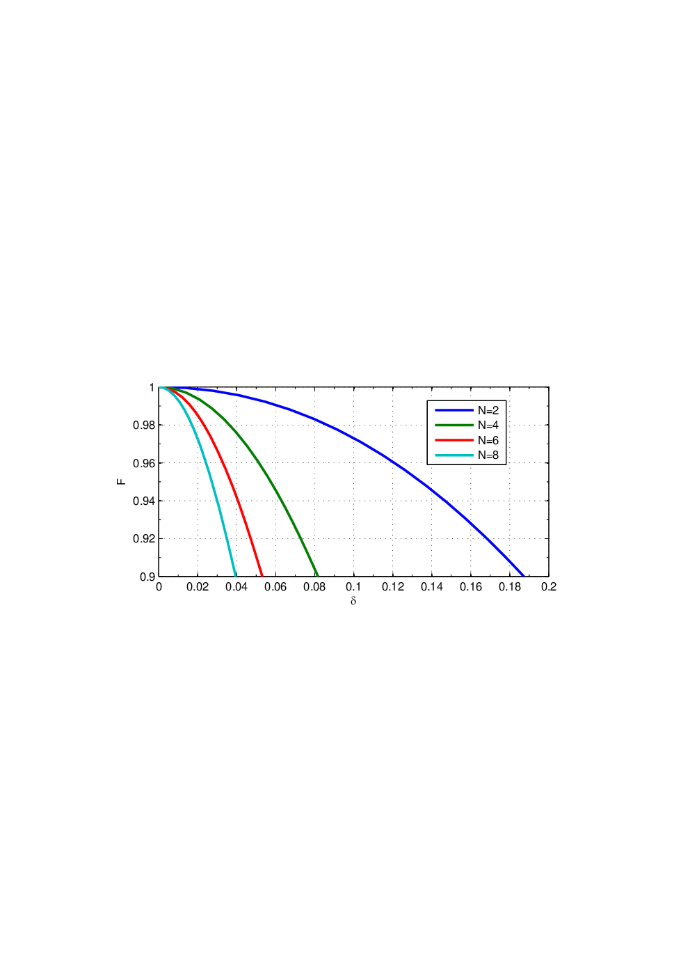
Figure 3 shows that the fidelity decreases as the error in the coupling coefficient increases. In the case of a 4-qubit GHZ state, a fidelity of can be achieved if the error in is within . However, as the number of qubits increases, the fidelity drops more rapidly. Hence a more precise control of the flux bias is required to realize many-qubit GHZ states.
IV Error caused by decoherence
An important advantage of our proposal is that the state preparation is independent of the initial state of the resonator. In general, it is not easy to prepare the system to be exactly in the ground state. For example, at typical dilution fridge temperatures, say mK, there is a non-negligible probability () for the first excited state of a GHz resonator to be occupied. This problem is less severe for the qubits since their energy scale is much higher. Therefore a scheme which is insensitive to the initial state is desirable.
Figure 2 shows the fidelity of the prepared GHZ state for two different initial states of the resonator (the ground state and the thermal state at mK). Although the time evolutions are different in general, the fidelities at the decoupling time (indicated by black dots in the figures) are the same. This can be explained from Eq. (14), at times , only the first term of Eq. (14) is kept, i.e., the qubits and resonator are decoupled. No matter what the initial state of the resonator is, at these times, the resonator has evolved back to its initial state. This means the GHZ state preparation is not influenced by the initial state, or in other words, the preparation is insensitive to the decoherence that occurred before the interaction was switched on.
But the decoherence during the operation certainly changes the final output state. In general, environmental fluctuations induce both dephasing and relaxation to the system. Since the qubits are all biased at the degeneracy point, the strong dephasing effect due to 1/f noise is largely suppressed. Thus we can use a master equation which only includes relaxation as damping instead of the unitary operator Eq. (14) to fully characterize the time evolution
| (33) |
where is the density matrix of the system (qubits + resonator) in the interaction picture and represents the decoherence of the resonator
| (34) |
Here, is the resonator decay rate and the average number of photons in the resonator. Finally, represents the decoherence of the qubits
| (35) |
where is the qubit decay rate and are written in the diagonal basis of . The quality factor of a TLR can be as high as than . The qubit -time at the degeneracy point is several s at most in present experiment. To be on the safe side, we assume for the resonator , MHz, and for the qubit ns, i.e., the decay rate is MHz. Here we neglect excitations of the qubit since its energy spacing is much larger than the thermal fluctuation. To investigate the influence of decoherence, we compare the fidelity to prepare a GHZ state with/without decoherence. The result is shown in Fig. 4 where the difference of the two fidelities (where is the fidelity in the presence of decoherence) is plotted as a function of time. The red dots mark the difference at the GHZ preparation times . Obviously, the error due to decoherence increases with time. As we analyzed in the previous section, the preparation time is much shorter than the decoherence time. Therefore the error is still quite small at the minimum preparation time (indicated by the first dot): the error caused by decoherence is around in the 4-qubit case.


V Discussion and Conclusion
In the above discussion, for simplicity, we assumed that the qubits only interact with a single mode of the resonator. However, since we did not invoke the rotating wave approximation in our calculation, higher modes of the TLR [20, 32] will also contribute to the coupling. Therefore, the interaction Eq. (13) should include a sum over multiple modes whose frequencies are below a cut-off . The cut-off is determined by a number of practical issues, e.g., by the superconducting gap, or the fact that the resonator is not strictly one-dimensional [20]. The time evolution including higher modes is of the same form as Eq. (14) but includes a product over all the relevant modes. Neglecting the small nonlinear effect due to output coupling, the frequencies of all higher modes are multiples of the frequency of the fundamental mode, and , all the coupling coefficients between the qubits and different modes of the TLR, are still zero for . Here . Hence the only correction to our scheme is including a sum over all the relevant modes in the definition of in Eq. (17),
| (36) |
For low excitation modes whose wave lengths are still much larger than the qubit dimension, the homogeneous coupling assumption still approximately valid, i.e., . For example, considering for a cm transmission line, around the center there is a mm-long region where the magnetic field varies within %. The distance between the center of two qubits is roughly m. This means up to around 30 qubits are coupled to the resonator approximately homogeneously. One can also tune to further compensate the slight inhomogeneity. The correction to the time evolution Eq. (22) can be simply written as . Therefore, the effect of the higher excitation modes actually amounts to increasing the coupling coefficient , which helps to reduce the operation time.
The electric field of the higher modes has little effect on the flux qubits but will change the voltage bias of the charge qubits and couple to their component. However, at the degeneracy point, where the free Hamiltonian is proportional to , these coupling terms are rapidly oscillating and are expected to have a small effect on the system. However, the situation is less advantageous than for flux qubits, and higher modes should be suppressed by choosing high fundamental mode frequencies in the charge-qubit case.
For a small number of qubits, an (lumped) LC circuit can also be used as a quantum bus [33, 34] to generate a GHZ state by following our scheme. In this case, only one single mode contributes.
In conclusion, we have proposed a scheme to prepare an -qubit GHZ state in a system of superconducting qubits coupled by a transmission line resonator. We have analyzed the preparation scheme for both charge qubits and flux qubits. With this method, a multi-qubit GHZ state can be prepared within the quantum coherence time. In the case of flux qubits that is especially favorable, the preparation time is two orders of magnitude shorter than the qubit coherence time. The preparation time can be reduced further if the coupling strength is increased to the ultra-strong coupling regime, where the coupling strength is comparable to the free qubit Hamiltonian. The preparation scheme is insensitive to the initial state of the resonator and robust to operation errors and decoherence. The coupling can be switched by dc pulses of finite rise and fall times without introducing additional errors. In addition, the scheme described in this paper utilizes a linear coupling which is intrinsically error-free if proper dc control is achieved. Due to all these advantages, this proposal could be a promising candidate for GHZ state generation in systems of superconducting qubits.
VI Acknowledgement
The authors acknowledge helpful discussions with A. Wallraff and Yong Li. This work was partially supported by the EC IST-FET project EuroSQIP, the Swiss SNF, and the NCCR Nanoscience.
References
- [1] Y. Makhlin, G. Schön, and A. Shnirman, Rev. Mod. Phys. 73, 357 (2001).
- [2] J. Q. You and F. Nori, Phys. Today 58, 42 (2005).
- [3] G. Wendin and V. Shumeiko, in Handbook of Theoretical and Computational Nanotechnology (ASP, Los Angeles, 2006).
- [4] J. Clarke and F. K. Wilhelm, Nature (London) 453, 2008 (2008).
- [5] M. Steffen, M. Ansmann, R. C. Bialczak, N. Katz, E. Lucero, R. McDermott, M. Neeley, E. M. Weig, A. N. Cleland, and J. M. Martinis, Science 313, 1423 (2006).
- [6] J. Plantenberg, P. C. d. Groot, C. J. P. M. Harmans, and J. E. Mooij, Nature 447, 836 (2007).
- [7] S. Filipp, P. Maurer, P. J. Leek, M. Baur, R. Bianchetti, J. M. Fink, M. Göppl, L. Steffen, J. M. Gambetta, A. Blais, and A. Wallraff, Phys. Rev. Lett. 102, 200402 (2009).
- [8] F. Plastina, R. Fazio, and G. Massimo Palma, Phys. Rev. B 64, 113306 (2001).
- [9] L. F. Wei, Y.-X. Liu, and F. Nori, Phys. Rev. Lett. 96, 246803 (2006).
- [10] F. Bodoky,and M. Blaauboer, Phys. Rev. A 76, 052309 (2007).
- [11] M. D. Kim and S. Y. Cho, Phys. Rev. B 77, 100508(R) (2008).
- [12] J. Zhang, Y.-X. Liu, C.-W. Li, T.-J. Tarn, and F. Nori, Phys. Rev. A 79, 052308 (2009).
- [13] A. Galiautdinov and J. M. Martinis, Phys. Rev. A 78, 010305(R) (2008).
- [14] B. Röthlisberger, J. Lehmann, D. S. Saraga, P. Traber, and D. Loss, Phys. Rev. Lett. 100, 100502 (2008).
- [15] B. Röthlisberger, J. Lehmann, and D. Loss, Phys. Rev. A 80, 042301 (2009).
- [16] C. L. Hutchison, J. M. Gambetta, A. Blais, and F. K. Wilhelm, Can. J. Phys. 87, 225 (2009).
- [17] A. Galiautdinov, M. W. Coffey, and R. Deiotte, arXiv:0907.2225.
- [18] F. Helmer and F. Marquardt, Phys. Rev. A 79, 052328 (2009).
- [19] L. S. Bishop, L. Tornberg, D. Price, E. Ginossar, A. Nunnenkamp, A. A. Houck, J. M. Gambetta, J. Koch, G. Johansson, S. M. Girvin, and R. J. Schoelkopf, New J. Phys. 11, 073040 (2009).
- [20] A. Blais, R. S. Huang, A. Wallraff, S. M. Girvin, and R. J. Schoelkopf, Phys. Rev. A 69, 062320 (2004).
- [21] A. Wallraff, D. I. Schuster, A. Blais, L. Frunzio, R. S. Huang, J. Majer, S. Kumar, S. M. Girvin, and R. J. Schoelkopf, Nature (London) 431, 162 (2004).
- [22] Y. Nakamura, Y. A. Pashkin, and J. S. Tsai, Nature (London) 398, 786 (1999).
- [23] J. E. Mooij, T. P. Orlando, L. Levitov, L. Tian, C. H. van der Wal, and S. Lloyd, Science 285, 1036 (1999).
- [24] T. P. Orlando, J. E. Mooij, L. Tian, C. H. van der Wal, L. S. Levitov, S. Lloyd, and J. J. Mazo, Phys. Rev. B 60, 15398 (1999).
- [25] F. G. Paauw, A. Fedorov, C. J. P. M. Harmans, and J. E. Mooij, Phys. Rev. Lett. 102, 090501 (2009).
- [26] Y. D. Wang, A. Kemp, and K. Semba, Phys. Rev. B 79, 024502 (2009).
- [27] J. Wei and E. Norman, J. Math. Phys. 4, 575 (1963).
- [28] K. Molmer and A. Sorensen, Phys. Rev. Lett. 82, 1835 (1999).
- [29] L. You, Phys. Rev. Lett. 90, 030402 (2003).
- [30] A. Uhlmann, Rep. Math. Phys. 9, 273 (1976).
- [31] R. Jozsa, J. Mod. Opt. 41, 2315 (1994).
- [32] M. Göppl, A. Fragner, M. Baur, R. Blanchetti, S. Filipp, J. M. Fink, P. J. Leek, G. Puebla, L. Steffen, and A. Wallraff, J. Appl. Phys. 104, 113904 (2008).
- [33] I. Chiorescu, Y. Nakamura, C. J. P. M. Harmans, and J. E. Mooij, Science 299, 1869 (2003).
- [34] J. Johansson, S. Saito, T. Meno, H. Nakano, M. Ueda, K. Semba, and H. Takayanagi, Phys. Rev. Lett. 96, 127006 (2006).