Generating on-the-fly large samples of theoretical spectra through -dimensional grid
Abstract
Many analyses and parameter estimations undertaken in astronomy require a large set () of non-analytical, theoretical spectra, each of these defined by multiple parameters. We describe the construction of an -dimensional grid which is suitable for generating such spectra. The theoretical spectra are designed to correspond to a targeted parameter grid but otherwise to random positions in the parameter space, and they are interpolated on-the-fly through a pre-calculated grid of spectra. The initial grid is designed to be relatively low in parameter resolution and small in occupied hard disk space and therefore can be updated efficiently when a new model is desired. In a pilot study of stellar population synthesis of galaxies, the mean square errors on the estimated parameters are found to decrease with the targeted grid resolution. This scheme of generating a large model grid is general for other areas of studies, particularly if they are based on multi-dimensional parameter space and are focused on contrasting model differences.
Subject headings
techniques: spectroscopic — methods: data analysisI. Introduction
Various analyses and parameter estimations performed in growing number of applications in astronomy require a large set of non-analytical, theoretical spectra, where each spectrum in-principle can be defined by multiple free parameters. In stellar population synthesis using the Bayesian approach [19, 16, 35, e.g.,], as many as theoretical spectra and the derived line indices are used in order to cover a wide range of star formation histories from early- to late-type galaxies. With about 5 or more free parameters, each theoretical spectrum is a single stellar burst defined by metallicity and age, superimposed at a given mass fraction on a spectral component with exponentially decreasing star formation rate characterized by the age of the oldest stars, e-folding time of star formation, and both spectral components could be dust-attenuated. Similarly, theoretical spectra are considered in parameter estimation on stellar spectra [e.g., 34, who considered a model defined by 14 parameters], and on H II regions [e.g., 27, who studied a model defined by 15 parameters]. One approach to prepare and manage a non-analytical model is to store all of the pre-calculated spectra, fixed at both the parameter choice and the parameter resolution. As models are becoming more sophisticated and are growing in varieties, however, updating and storing or more spectra may not be the most flexible approach for many astronomers. To handle large sets of theoretical spectra at multi-dimensional parameter space is therefore a question that cannot be neglected.
We consider here current integrated stellar population models as a case study. These models, together with parameter estimation techniques or other analyses, were shown by many authors to be invaluable for deriving composition and star formation rate/history of different types of galaxies through their observed spectra, regardless whether or not a large model grid is used [37, 32, 19, 30, 18, 10, 38, 4, 11, 16, 25, 29, 31, 3, 36, 9, 33, e.g.,]. Firstly, there is a variety of spectral synthesis computational programs which use different flavors in initial stellar mass function, stellar types, and/or stellar evolutionary tracks [15, 24, 5, 26, 12, e.g.,]. The variations in input ingredients exist not only among the models, but also within a single model in the form of additional freedom in parameter choice. Secondly, increasingly more parameters are being included in the analyses, meaning that the parameter space defining the theoretical spectra is getting larger. So much so that Lee et al. [23] have recently constructed a stellar population model to the level of individual element abundances, with the goal to understand the effect of each and every element to the integrated spectrum of a stellar population. However, there are very few studies in the astronomy literature which address the case where a multi-dimensional parameter space defines a model. Two of the fundamental questions are: (1) how do we obtain, or interpolate, a theoretical spectrum in-between the parameter values, that is originally unavailable? (2) what is the best way for such an interpolation, taking into account of the noise in the data, and the possible non-linear dependence [39] between the theoretical spectrum and its underlying physical parameters? One of the goals of this work is to address the first question.
Here we describe a novel approach which increases the flexibility of handling a large set () of theoretical spectra, and is general for -dimension (D) parameter space. The approach adopts a hypercube, an D analog of a cube of length unity for each side [2, e.g.,], to represent the parameter space underlying each and every theoretical spectrum. The spectrum at any intermediate parameter point is generated on-the-fly11 1 We refer the on-the-fly ability to be the generation of theoretical spectra at run time as required by the actual computation, e.g., in parameter estimation. through multi-linear interpolation, upon an initial model grid that is designed to be lower in parameter resolution and therefore can be updated efficiently. We examine a pilot case in stellar population synthesis of galaxies, to show that the approach is applicable to studies in astronomy, and well manageable by a typical personal computer – a computer with Intel(R) Pentium(R)D 3.20 GHz CPU and 3.19 GHz RAM is used in this work.
All of the spectra considered in this work are expressed in vacuum wavelength, and are re-sampled to within the optical wavelength range Å at a resolution of 1 Å per wavelength bin. The Cartesian coordinate system is used throughout this work in representing the parameter space.
II. Method: An -dimensional grid for model parameters
Several desirable characteristics are identified in the setup for generating a large model grid: (1) generality for D parameter space; (2) the theoretical spectra defined by the targeted parameters are generated on-the-fly, which is essential for improving flexibility and saving disk space, especially in arbitrarily complex models; (3) targeted parameters can be specified at arbitrary position in the parameter space at run time, with the goal to obtain in the analysis/parameter estimation an arbitrary computational resolution which is limited only by the parameter resolution in the initial model grid.
To fulfill the above criteria, we generate a small- to moderate-size sample of theoretical spectra to start with. The underlying parameters of this initial sample is in the form of a Cartesian grid. For each parameter the size of the bins is allowed to be uneven, in which case the grid will be rectangular instead of square in the 2D analogy. For convenience we called this sample the initial grid of theoretical spectra, the purpose of which is to form a leverage for generating a larger sample of spectra, the targeted sample, for which the defining parameters can be located anywhere in-between the initial grid points. If this sample is also decided to be described by a parameter grid instead of random points within the initial grid, we called that the targeted grid of spectra. The advantage of having a targeted grid of sample is their offering an intuitive setting for performing necessary integrations over a parameter space in the applied parameter estimation technique, an approach also used by various authors [13, 19, 16, 40, e.g.,].
The theoretical spectrum at any intermediate grid point is calculated by first locating the corresponding neighboring spectra from the initial grid. The neighboring parameter grid points are then mapped into the corners of a hypercube of dimension , where is the number of parameters defining both the initial and targeted grids. The details of constructing a hypercube is described in §II.1. Multi-linear interpolation (described in §II.2) is next used to derive the concerned theoretical value at the targeted parameter point. The value is, in the current context, the flux density in a given wavelength bin. Therefore, the above procedure is repeated for each and every wavelength bin of interest. The whole procedure of model generation is joined seamlessly with the actual computational routines for parameter estimation or other analyses, with the only input being the initial model grid.
II.1. Hypercube
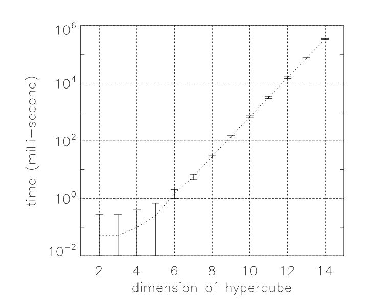
A hypercube is an D cube with each side equals unity. In 2 and 3 dimensions, a hypercube is hence a square and a cube, respectively. This geometry makes a hypercube to be naturally suitable for describing an D Cartesian space, such as a grid of model parameters. For our purpose, the dimension of the parameter space is defined to be the number of parameters that fully specifies a spectrum. For example, in a simple stellar population defined by stellar age and stellar metallicity, = 2. In practice, a hypercube is generated by specifying all the corners using vectors, or arrays in the actual computational routines. For example, in 2D the arrays are and , where any coordinate value is defined to be either 0 or 1. It is easy to show by deduction that there are in total corners in an D hypercube.

We use a random rendering of points, together with a book-keeping approach, to create each and every corner of the hypercube exactly once. After some algebraic derivations in the low-dimensional cases, we found that the number of combinations – or the number of corners – in the hypercube of dimension , for occurrences of 1’s in the array specifying the corner is given by the binomial coefficient
| (1) |
In 3D, there is 1 () combination of no 1: , 3 () combinations of one 1: , and , 3 () combinations of two 1’s: , and , and 1 () combination of three 1’s: . Other approaches certainly can be used to accomplish the same purpose, as long as a hypercube is automatically created given only its dimensionality, .
The time required to construct a hypercube of a given dimension is shown in Figure 1. For dust-attenuated integrated stellar spectra defined by an exponentially decreasing star formation rate, = 4 (age, , , , at fixed initial stellar mass function and other parameters), the time is less than 1 milli-second. For an extra dust-attenuated stellar burst which is added at a certain flux fraction, = 8 (age, , and the burst mass relative to the total galaxy mass), the time is less than 1 second. The construction of the hypercube therefore should not constitute as bottleneck in typical analyses or parameter estimation problems, which take minutes to hours of computation.
II.2. Multi-linear interpolation at intermediate grid point
To interpolate a spectrum at an intermediate parameter point in the initial grid, called the targeted point, we first perform a search to locate all of points, or the neighboring points, from the initial grid that encloses the targeted point. This search is performed on the parameter-to-parameter basis, for each parameter a pair of neighboring points is obtained. As a result, the searching time scales as and is quick in typical applications, where is the number of grid points for a given parameter. Next, we map the corners of a hypercube to these neighboring points, in total for an D hypercube.
The weight of the theoretical value of a grid parameter point to that in the targeted parameter point is illustrated in Figure 2, in the 2D case. The weight of point to the targeted point is the area of the stippled square, . When the point coincides with , , or the weight on the targeted point value due to point is zero. The final interpolated value at the targeted point is calculated by summing up contributions from all of the points
| (2) | |||||
For a square of unit length for each side, we can re-write to be , similarly for other corners.
To extend to the D parameter space, the interpolation formula for the value of interest at the targeted point , , is
| (3) |
where denotes the sum over contributions from all of the neighboring points, , enclosing the targeted point, , and the weight of each neighboring point is
| (4) |
in which denotes a given parameter axis in the D parameter space. For a hypercube of length unity for each side, is equal to unity. This formula is an extension of linear interpolation in the 1D case by Burnett [6, his Eqn. 5.2], and is shown to be applicable to computations in fluid dynamics [28].
The Eqns. 3 and 4 assume normalized coordinates, as such the range of each coordinate value lies within . Since the neighboring points are represented by the corners of a hypercube, no extra normalization step is required for those. The target point is normalized according to
| (5) |
where is the actual parameter value (e.g., age = 3 Gyr) at point , and and are that of the pair of neighboring points enclosing the targeted point, for the -th parameter axis (e.g., age = 1 Gyr and 4.2 Gyr, respectively). To derive the flux densities of a targeted spectrum, Eqns. 3 and 4 are applied on the wavelength-to-wavelength basis. If the uncertainty in the flux density of the theoretical spectra is also available, Eqn. 3, together with usual error propagation formulae, can be used to obtained the uncertainty in the interpolated spectrum.

The accuracy of the interpolated value at an intermediate parameter point in-between the initial grid points depends on how good the linearity assumption is. This simplifying assumption is made only locally, i.e., in-between two grid points in the initial parameter grid, for a given parameter axis. There is no requirement that the linearity has to stand in the global range of a parameter. The reason is that any non-linear change of the theoretical value with parameter globally can be taken into account, e.g., by adopting a higher sampling fraction of the initial grid points in the related parameter regions. If indeed the spectral features depend highly non-linearly with parameters that happen to occur at unknown parameter amplitude(s), a preliminary step can be taken to locate the concerned parameter amplitudes. The recently introduced locally linear embedding [39] appear to be a promising approach for this purpose, for its ability to unfold a non-linear manifold (see their Figure 1).
III. Effect of Grid Resolution on Parameter Estimates
A fundamental aspect in parameter estimation is the choice of grid resolution. A finer parameter grid is expected to give higher accuracy in the estimates, whereas a smaller one requires less computational time. We use here the on-the-fly ability of our model generation approach to investigate the effect of the targeted grid resolution on the parameter estimates. This study requires multiple sets of models of increasingly large sample size.
To construct an initial grid we use the Bruzual & Charlot [5] stellar population model (resolution 1 Å per wavelength bin within the vacuum wavelength range Å), and the Calzetti et al. [7] intrinsic dust model. The initial stellar mass function is that by Chabrier [8] [similar to 22, with a turnover below ] with lower and upper limits in stellar mass, . A wide range of stellar population and dust parameters is covered – the age of the oldest stars, age, takes the values: Gyr, stellar metallicity, : , the e-folding time of an exponentially decreasing star formation history, : Gyr and the color excess, : mag. The resultant (4D) initial model grid is consist of 625 dust-attenuated integrated stellar spectra. The initial grid is fixed throughout the analysis.
An example interpolated spectrum is shown in Figure 3. Its age, , and are respectively 8 Gyr, 0.02, 9 Gyr, 0.3 mag. The difference spectrum, interpolated - true theoretical spectra, is also shown. The true theoretical spectrum is referred to that being output directly from the Bruzual & Charlot [5] program, and post dust-attenuated with the Calzetti et al. [7] model. The flux density error is driven by both the parameter resolution in the initial grid and the validity of the linearity assumption within a single bin of the initial grid. In the interpolated spectrum, the error is about 2%, assigned equally to each and every wavelength bin to give a reduced between the two spectra close to unity (equals in this case). Extending to the full parameter space, we generate 320 spectra at age = Gyr, = 22 2 The stellar metallicity values chosen here are not different from those in our initial grid, because other metallicity values are not output directly from the Bruzual & Charlot [5] program. So in this example we are in fact considering a 3D interpolation in a 4D hypercube., = Gyr and = mag using the above-mentioned initial grid, which are compared with the true theoretical spectra. Figure 4 shows the distribution of the flux density error in the interpolated spectra, showing an average of , a minimum of , and a maximum of ; with a resultant average of . The amplitude of the flux density error is comparable with, e.g., the spectrophotometric uncertainty from the Sloan Digital Sky Survey Data Release 6, 7% in the observed frame wavelength of 3800 Å [1]. The threshold in the flux density error, at which the interpolated spectrum is still useful, would depend on individual applications. We plan to extend this type of comparison to other models. One model to consider, e.g., is that by Kotulla et al. [21], who provide an interactive web interface for downloading theoretical spectra of integrated stellar systems which are defined by multiple parameters.

We next construct a mock galaxy sample for the parameter estimation, in which the parameters underlying each spectrum are known. Based on the initial grid, a random sample of 100 theoretical spectra are generated through our approach. Random Gaussian noise is added to the flux density in each wavelength bin of each spectrum, fixed at signal-to-noise () of 20. Bayesian parameter estimation is then performed on the mock sample, using the approach described by Kaviraj et al. [20], where all of the 4 model parameters are estimated simultaneously. The parameter estimations are carried out using several different samples of theoretical spectra, defined from high to low parameter resolution, as shown in Table 1. These spectra are also generated using the model generation approach described in this work, and are based on the same initial grid. As such, we are probing the effect on the parameter estimates due to the increasing targeted grid resolution only, rather than that due to model imperfection in terms of describing the real observed spectra, and so on. Except for the stellar metallicity, for which we follow Gallazzi et al. [16] and adopt logarithmic bins (i.e., evenly sized in ), linear bins (i.e., evenly sized bins) are used for all of the other parameters (age, and ) in the targeted grid.
| Targeted grid size | Reduction factor | Number of spectra |
|---|---|---|
| 14 36 15 17 | 1 | 128520 |
| 10 24 10 12 | 1.5 | 28800 |
| 7 18 8 9 | 2 | 9072 |
| 4 9 4 5 | 4 | 720 |
There are 4 parameters (age, , , ) constituting each of the grids, in that order the grid size is given. The range of a parameter is the same for all of the grids, given in §III. The reduction factor is the approximate fractional decrease of grid resolution relative to the case of highest resolution, and is set to be uniform in each parameter. Except in for which logarithmic bins are adopted, linear bins are used in all of the other parameters.
The dependence of the root mean square error (RMSE), the square root of the variance and the bias (the average difference between the estimate and the true parameter value) of the estimated parameter are shown in Figure 5, for each of the parameters. Mathematically, the RMSE is the square root of the mean square error (MSE). The MSE is the sum of the variance and the bias squared, so it can be interpreted as the sum of the squares of statistical and systematic errors [14]. The MSE is found to decrease as the resolution of the targeted parameter grid increases, an indication of an improved determination of the posterior probability for each parameter of the mock galaxies, in this case, due to the increase in the number of parameter grid points being sampled. We also see that the estimates are fairly unbiased when the number of theoretical spectra for our parameter ranges, where the corresponding grid resolution is listed in Table 1. On the other hand, the variance of the estimates at our large-sample limit should be limited by the data . For example, Gallazzi et al. [16] compared (their Figure 3) both the shape and the width of the posterior probability in stellar metallicity between the high- and low- spectra from the Sloan Digital Sky Survey [42], in that lower spectrum gives wider distribution in the posterior probability of parameters. Earlier Gil de Paz & Madore [17] also came to similar conclusion, through parameter recovery test upon synthetic photometry of integrated stellar populations.


Another interesting aspect of Figure 5 is the simultaneous improvement in all of the parameter estimates upon the increase in the targeted parameter grid resolution. This result manifests the presence of degeneracies among all of the involved parameters – age, , and . It is well-known that age-metallicity degeneracy may hinder the studies of astrophysical objects by using only their broadband colors. Even integrated spectra are not immune from this degeneracy – an integrated stellar spectrum with intermediate to old age (1.5 Gyr and up) may look the same by tripling the age or reducing the stellar metallicity by a factor of two [41]. To determine age, one therefore needs to know , and vice versa, meaning both parameters have to be determined simultaneously. Figure 5 demonstrates that degeneracies exist among all of the considered parameters, in the way that the improvements on these estimates go hand-in-hand.
IV. Summary
In applications where a large (sample size ), non-analytical model is needed, the hypercube representation of the parameter space, together with multi-linear interpolation for deriving the theoretical value at an intermediate grid point, are shown here to be feasible to improve the flexibility in handling the models. Using stellar population synthesis of galaxies as a pilot study, we found that the increase in targeted parameter grid resolution improves the parameter estimates in terms of the mean square error. This example is given by incorporating the Bayesian parameter estimation. Naturally, our model generating approach can be combined with other parameter estimation techniques, such as the Markov Chain Monte Carlo.
Models of large sample size can be applied to studies in various areas and disciplines. In the context of spectral analyses, a large grid of theoretical spectra is expected to be applicable to mock catalog construction, studying the relationship between spectral features and model parameters, spectral fitting, and stellar population synthesis of galaxies. Our approach is particularly suitable for studies that are based on multi-dimensional parameter space, and are focused on investigating differences among results obtained through different models.
V. Acknowledgments
I thank Rosemary F. G. Wyse for discussions which lead to this work, and her comments on the manuscript. I thank Tamás Budavári and Andrew Ptak for discussions on parameter estimations, and Sandra Faber for discussions on relating spectra to physical parameters. I thank Niraj Welikala and Alex S. Szalay for various discussions. I thank the referee for useful comments and suggestions. I acknowledge support through grants from the W. M. Keck Foundation and the Gordon and Betty Moore Foundation, to establish a program of data-intensive science at the Johns Hopkins University.
This research has made use of data obtained from or software provided by the US National Virtual Observatory, which is sponsored by the National Science Foundation.
References
- [1] Adelman-McCarthy, J. K., et al. 2008, ApJS, 175, 297
- [2] Anthony, M. 1987, Discrete Mathematics of Neural Networks: Selected Topics, Society for Industrial Mathematics
- [3] Asari, N. V., Cid Fernandes, R., Stasińska, G., Torres-Papaqui, J. P., Mateus, A., Sodré, L., Schoenell, W., & Gomes, J. M. 2007, MNRAS, 381, 263
- [4] Brinchmann, J., Charlot, S., White, S. D. M., Tremonti, C., Kauffmann, G., Heckman, T., & Brinkmann, J. 2004, MNRAS, 351, 1151
- [5] Bruzual, G., & Charlot, S. 2003, MNRAS, 344, 1000
- [6] Burnett, D. S. 1986, Finite Element Method, Addison-Wesley Pub. Co., Reading, MA
- [7] Calzetti, D., Armus, L., Bohlin, R. C., Kinney, A. L., Koornneef, J., & Storchi-Bergmann, T. 2000, ApJ, 533, 682
- [8] Chabrier, G. 2003, PASP, 115, 763
- [9] Chen, Y.-M., Wild, V., Kauffmann, G., Blaizot, J., Davis, M., Noeske, K., Wang, J.-M., & Willmer, C. 2009, MNRAS, 393, 406
- [10] Cid Fernandes, R., Gu, Q., Melnick, J., Terlevich, E., Terlevich, R., Kunth, D., Rodrigues Lacerda, R., & Joguet, B. 2004, MNRAS, 355, 273
- [11] Cid Fernandes, R., Mateus, A., Sodré, L., Stasińska, G., & Gomes, J. M. 2005, MNRAS, 358, 363
- [12] Coelho, P., Bruzual, G., Charlot, S., Weiss, A., Barbuy, B., & Ferguson, J. W. 2007, MNRAS, 382, 498
- [13] Conti, A., et al. 2003, AJ, 126, 2330
- [14] Cowan G. 1998, Statistical Data Analysis, Clarendon Press, Oxford
- [15] Fioc, M., & Rocca-Volmerange, B. 1997, A&A, 326, 950
- [16] Gallazzi, A., Charlot, S., Brinchmann, J., White, S. D. M., & Tremonti, C. A. 2005, MNRAS, 362, 41
- [17] Gil de Paz, A., & Madore, B. F. 2002, AJ, 123, 1864
- [18] Glazebrook, K., et al. 2003, ApJ, 587, 55
- [19] Kauffmann, G., et al. 2003, MNRAS, 341, 33
- [20] Kaviraj, S., Rey, S.-C., Rich, R. M., Yoon, S.-J., & Yi, S. K. 2007, MNRAS, 381, L74
- [21] Kotulla, R., Fritze, U., Weilbacher, P., & Anders, P. 2009, MNRAS, 396, 462
- [22] Kroupa, P., Tout, C. A., & Gilmore, G. 1990, MNRAS, 244, 76
- [23] Lee, H.-c., et al. 2009, ApJ, 694, 902
- [24] Leitherer, C., et al. 1999, ApJS, 123, 3
- [25] Mathis, H., Charlot, S., & Brinchmann, J. 2006, MNRAS, 365, 385
- [26] Maraston, C. 2005, MNRAS, 362, 799
- [27] Morisset, C. 2009, MmSAI, 80, 397
- [28] Murman, S. M., Aftosmis, M. J. & Nemec, M. 2004, NAS Technical Report NAS-04-015, November
- [29] Ocvirk, P., Pichon, C., Lançon, A., & Thiébaut, E. 2006, MNRAS, 365, 74
- [30] Panter, B., Heavens, A. F., & Jimenez, R. 2003, MNRAS, 343, 1145
- [31] Panter, B., Jimenez, R., Heavens, A. F., & Charlot, S. 2007, MNRAS, 378, 1550
- [32] Reichardt, C., Jimenez, R., & Heavens, A. F. 2001, MNRAS, 327, 849
- [33] Richards, J. W., Freeman, P. E., Lee, A. B., & Schafer, C. M. 2009, MNRAS, 1327
- [34] Robitaille, T. P., Whitney, B. A., Indebetouw, R., & Wood, K. 2007, ApJS, 169, 328
- [35] Salim, S., et al. 2007, ApJS, 173, 267
- [36] Tojeiro, R., Heavens, A. F., Jimenez, R., & Panter, B. 2007, MNRAS, 381, 1252
- [37] Trager, S. C., Faber, S. M., Worthey, G., & González, J. J. 2000, AJ, 119, 1645
- [38] Tremonti, C. A., et al. 2004, ApJ, 613, 898
- [39] Vanderplas, J., & Connolly, A. 2009, AJ, 138, 1365
- [40] Welikala, N., Connolly, A. J., Hopkins, A. M., Scranton, R., & Conti, A. 2008, ApJ, 677, 970
- [41] Worthey, G. 1994, ApJS, 95, 107
- [42] York, D. G., et al. 2000, AJ, 120, 1579