QCD: The as a Hybrid
Abstract
Using the QCD Sum Rule Method, we estimate the mass of the lowest strange mixed hybrid/three-quark baryon with . We find the mass for a hybrid is approximately that of the , whose nature has been a puzzle for many decades. Possible tests of this result are discussed.
1 Introduction
The nature of the has been of interest for many years. More than four decades ago experiments showed[1] that this was a state with spin=1/2. Using a SU(3) meson-baryon potential it was predicted to be a resonance[2, 3] with . There have been many studies using such a model. Recently chiral SU(3) meson-baryon potentials have been used in detailed studies[4, 5], and conclude that the the is a resonance. See Refs.[4, 5] for references to earlier publications using such a model. Recent experiments using the CLAS detector system at JLAB have carried out high statistics photoproduction measurements of the [7]. Although the analysis of the data is not complete, the present results do not seem to be consistent with resonance models.
Recently, the method of QCD Sum Rules has been used to explore the possibility that the has a large pentaquark component[6]. As explained in Ref[6], the results are not conclusive; and the authors also discuss attempts by other authors to find the nature of the . These theoretical models and experiments have shown that the is not a standard three-quark baryon, and are the motivation for our present work, in which we explore the possibility that the is a strange hybrid baryon.
For many decades there has been a great interest in detecting and studying hybrid hadrons. The early work on hybrid hadrons was based on quark models, in which mesons with certain so-called exotic quantum numbers could not exist as quark-antiquark states. Since with three quarks there are no such exotic quantum numbers, all of the work was on mesons as quark-antiquark-gluonic states. See Ref[8] for a review of hybrid mesons using bag models.
At the present time by hybrids one uses the concepts of Quantum Chromodynamics (QCD) in which the quarks are in a color octet, and with a color octet valence gluon form a color singlet physical state. Therefore, hybrids can be mesons or baryons. With such a hybrid theory the would have three quarks (uds) in an octet configuration and a valence octet gluon. Thus it would have a [udsg] structure. There have been a number of studies of the as a strange hybrid. In recent studies by Kittel and Farrar[9, 10] using the bag model of Barnes and Close (who also studied the [11, 12]) the isosinglet and (with ) were found to be hybrids. This model, however, is not consistent with the negative parity of the . Note that in the earlier work with this model[12] the lightest possible hybrid was found to be , and a mass of 1405 was ruled out.
Soon after the method of QCD Sum Rules was introduced it was used to study hybrid mesons[13, 14]. Recently a study of vector states found[15] hybrid mesons with masses 2.3-2.6 GeV. Some years ago a calculation using QCD Sum Rules was carried out to find lightest hybrid baryon with , like the proton[16]. This was followed by an improved calculation[17], with the result that the mass of this hybrid is approximately that of the , the Roper resonance. The Roper is a very broad resonance, and there might even be two states, a hybrid and a non hybrid. An extension of this work, that is closely related to our present project, was the use of QCD Sum Rules to find the lowest strange hybrid baryon[18]. Such a state was found at the energy of the , about 500 MeV above the , which allows a possible experimental test via decay. We shall discuss this below.
Recently studies of heavy quark hybrids were carried out. It was shown that there is no satisfactory solution for hybrid charmonium or upsilon in the lowest energy states[19]. In a subsequent study[20] it was shown that the and states are approximately 50-50 mixtures of hybrid and normal mesons. This provides a solution to some puzzles in the decays of these states that standard quark models, which can fit the energies of the states as pure heavy quark mesons, cannot explain.
In the present research we extend the work of Ref[17], first using a current for a strange hybrid baryon, an then a current with mixed hybrid and normal three-quark strange components. Our objective is to find the mass of the lowest mixed strange hybrid/three-quark baryon, to see if our solution satisfies the conditions for a satisfactory QCD Sum Rule solution, and to compare it to the mass of the . We then discuss some possible experimental tests of the as a hybrid, incluidng photoproduction.
2 as a hybrid
Following the work of Ref.[17], in which QCD Sum Rules were used to show that there is a hybrid baryon with the quantum numbers of the proton and the Roper resonance, with a mass about that of the Roper resonance, we investigate the possibiity that the is a hybrid baryon. Also, recently it has been shown that although the is not a hybrid meson, it is a mixed hybrid-charmonium meson, with a similar result for the , which solves some puzzles[20]. In our present work we attempt to find the lightest hybrid with the properties of the ; and if it turns out that there is no satisfactory solution, in future work we shall explore the possibility that the is a mixed hybrid-normal baryon.
The current that we use for a strange hybrid baryon is that used in Ref.[17] with modifications for the quantum numbers of the . The current for the baryon[21], expressed in a more convenient form[22]
| (1) |
Using the same modification as for a hybrid nucleon[17], the current that we use for a strange hybrid is
| (2) |
In Eq(2) a,b,c are color indices and u, d, s are up, down, and strange quark fields; and
| (3) |
with the SU(3) generator ().
First we shall use the method of QCD Sum Rules to estimate the mass of the lowest strange hybrid baryon and see if it matches the mass of the . Then we shall use a current which is an admixture of a hybrid and a normal strange baryon.
2.1 Review of QCD Sum Rules for a strange hybrid baryon
The correlator for use in the QCD sum rule method for a strange hybrid baryon with is
| (4) |
The QCD sum rule method is based on equating a dispersion relation of the correlator, called the left hand side, to an operator product expansion (OPE) of the correlator, called the right hand side. For our hybrid hypothesis the dispersion relation is
| (5) |
where is the mass of the state (assuming zero width) and is the start of the continuum–a parameter to be determined. The imaginary part of , with the term for the state we are seeking shown as a pole (corresponding to a term in ), and the higher-lying states produced by shown as the continuum, is illustrated in Fig. 1

Next is evaluated by an operator product expansion (O.P.E.), giving the right-hand side (rhs) of the sum rule
| (6) |
where are the Wilson coefficients and are gauge invariant operators constructed from quark and gluon fields, with increasing corresponding to increasing dimension of . It is important to note that the Wilson coefficients, obey renormalization group equations[22]
After a Borel transform, , in which the q variable is replaced by the Borel mass, , the final QCD sum rule has the form
| (7) |
For a succesful solution the value of should have a minimum near the value of , and should not depend very much on . Also, the value of should be approximately the magnitude of the square of the mass of the next higher excited state.
2.2 QCD Sum Rule for a Strange Hybrid baryon.
It is useful to divide the correlator into a vector and scalar part, and :
| (8) |
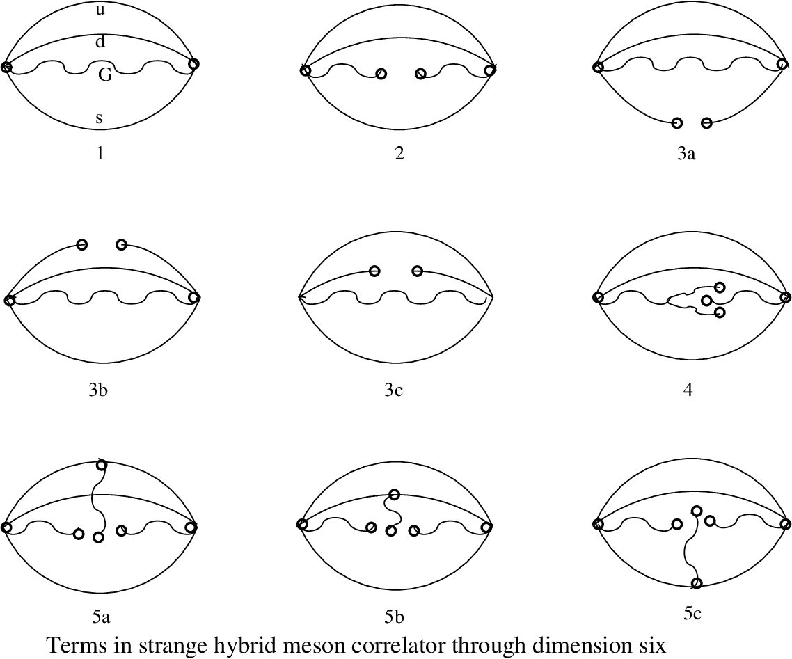
For our present problem we use diagrams up through dimension six. The diagrams needed are shown in Fig.2.
The lowest dimension term, shown as 1 in Fig. 2, is
| (9) | |||||
with the f-flavor quark propagator. Neglecting the quark masses for the u and d quarks, the quark propagators are
| (10) | |||||
where is the strange quark mass, and we assume for the values of which are relavent for the calculation of the mass of the hybrid baryon.
Thus for the vector part of one must evaluate
| (11) | |||||
We do not need the scalar part, , as is explained below.
In order to complete the calculation of one needs the following:
| (12) | |||
After a rather complex calculation, using , we find that
| (13) |
The next term in the OPE, shown as 2 in Fig. 2, contains the gluon condensate. The basic difference from diagram 1 is[22]
| (14) | |||||
where is the gluon condensate. This term of the correlator has only a vector part, and in momentum space is
| (15) |
The quark condensate terms are shown as diagrams 3a, 3b and 3c, Fig. 2. Processes 3b and 3c vanish, while 3a is obtained from process 1 with the replacement (see Eqs.(9,10))
| (16) |
where is the strange quark condensate. Therefore we find that processes 3 have only a scalar part, and in momentum space is
| (17) |
For process 4, Fig. 2, one makes use of the OPE for the gluon field[22]:
| (18) | |||||
where the first term gives the gluon condensate in process 2.
To obtain the correlator for process 4 one needs the expression for the three-gluon vacuum expectation value:
| (19) |
with the six-dimensional three-gluon condensate.
After a complicated calculation one finds for the vector correlator for process 4
| (20) |
The final dimension six processes are shown in diagrams 5a, 5b, and 5c, FIG. 2. One can show that the sum of the two terms with gluon fields coupled to the u and d quarks, processes 5a and 5b, cancel; i.e., . For the 5c process, with a gluon field coupled to the strange quark, the calculation is similar to the calculation for process 2, with a gluon condensate, with the propagator for the s quark replaced by the s quark propagator with an external gluon field, as shown in process 5c of Fig. 2. Thus the expression for the s quark propagator becomes
| (21) |
After a lengthy calculation one finds for the vector part of process 5 in momentum space
| (22) |
The only nonvanishing mixed quark condensate only contributes to the scalar part of the correlator, like process 3, which does not enter in our estimate of the strange hybrid mass (see below), and is therefore not considered. The final dimension six diagram is the four-quark condensate, proportional to . Using one finds that this diagram is less than 10 % of the leading diagram, and is neglected.
In summary, separating the hybrid correlator into a vector and scalar part, with the vector part
| (23) |
| (24) | |||||
We use the standard values for the gluon condensates, = 0.0377 GeV2 and = 0.0422 GeV6, with . Note that in Refs[19, 20] only the scalar part of the correlator is used to estimate the hybrid meson mass. The vector correlator is more reliable for the present calclculation, as the scalar part mainly has higher dimensional contributions, and we only use the vector correlator to estimate the strange hybrid mass in our present work. In many applications of the QCD Sum Rule Method one obtains the mass of the pole term by taking the ratio of the vector to scalar correlator, or similar techniques. This removes unknown constants. Another standard technique is to use either the vector or scalar component and take the ratio to the sum rule to its derivative with respect to , which is the method we use in the present work.
First note that the Borel transform has the following properties:
| (25) |
From this we obtain the left and right hand sides of the correlator as a function of the Borel mass (in units of GeV):
| (26) | |||
where is the amplitude of the pole term, the are chosen to fit the continuum, and is the value of at the start of the fit to the continuum.
Evaluating the sum rule by combining it with a derivative of the sum rule (see, e.g., Ref[20]), and redefining the constants , one obtains the expression for as a function of
| (27) | |||||
The solution to the sum rule is shown in FIG 3. Following the standard QCD Sum Rule procedure, the parameters are chosen so the value of has a minimum and has a very weak dependence on in the region of the minimum. The solution shown in FIG 3 is obtained with =2.5 GeV2 and , with appropriate powers of GeV.

With =2.5 GeV2 and the values of given above, the pole term approximately 40% larger than the continuum. This satisfies the criteria for a good solution. Using the criteria that have been used for decades we estimate that the error in our calculation of the mass is about 15 per cent. As one can see from the figure the mass of the lowest strange hybrid with is 1407 MeV, which is approximately the mass of the . We emphasize that by including all graphs through dimension six, we ensure the convergence of the operator product expansion. Note that the dimension six contributions to the correlator after the Borel transformation are very small.
In thre next section we consider a mixed hybrid-three quark model for the .
3 as a mixed hybrid/3-quark strange baryon
In our study of heavy quark mesons[19], no hybrid charmonium solution was found; and in further studies of charmonium and upsilon states it was shown[20] that the and states are a mixed hybrid and normal meson. In the study of the by Nakamura [6] QCD Sum Rules were used with a mixed three-quark () and pentaquark () current. Although a stable solution was not found, this study showed that the 3-quark component was small. We now investigate the possibility that there is a QCD Sum Rule solution with a correlator given by a mixed hybrid and 3-quark current:
| (28) |
and the correlator
| (29) | |||||
Where is the hybrid current, defined in Eq(2) and is the three-quark current.

We could use the same for a strange state as in Ref[6], but since it has different dimensions than for our calculation or with a mixed and , current, the Sum Rule method cannot be used without a method of normalizing the two components of the current. In Ref[6] a model for the wave functions was used to obtain the dimensional normalization. In our present work we wish to use QCD direclty. Using the method derived for the mixed heavy-quark/hybrid-heavy-quark QCD Sum Rule calculation[20] we obtain a crucial relationship between and correlators, which are shown in Fig 4.
By using the external field method, as in Ref[20] one can show that
| (30) |
Noting that and have the same dimension, we use for the mixed hybrid/3-quark strange correlator
| (31) |
Note that there are three diagrams for , shown in Fig.4b. The gluon from the hybrid vertex can couple to the u, d, or s quark. The first two cancel, and is given by the coupling to the strange quark:
| (32) |
All of the quantities in Eq(32) have been defined above except the anticommutator , and .
After a somewhat complicated calculation and a Fourier transform, we find that with the neglect of quark masses, as in the calculation of , the only term with dimension 6 or less has the form , proportional to the second term in shown in Eq(26). Therefore, after a Borel transform will be proportional to as is the second term in , Eq(26). One finds (in comparison to the second term in , ) that
| (33) |
Thus we find that the contribution to the mixed hybrid/3-quark correlator from the 3-quark component is approximately 20 % of the second-order term in the hybrid correlator for any value of b. Noting that terms of this magnitude have been dropped in obtaining the hybrid correlator, as discussed in Section 2, we conclude that our calculaion of the as a hybrid, discussed in the previous section, is unchanged within errors of the method of QCD Sum rules. Our result is analogous to that in Ref[6] in which it was found that the 3q component was very small in their 3q/5q model.
It is interesting to compare our present calculation of the as a mixed mixed hybrid/3-quark state to our previous calculation of the Roper as a mixed hybrid/3-quark state, with the 3-quark component being nucleon-like. In that calculation[17] it was found that the 3-quark component of the Roper was small, and that the Roper is essentially a pure hybrid baryon, similar to our conclusion about the nature of the .
We now discuss possible experimental tests of the hybrid nature of the .
4 Experimental tests of the as a hybrid
The only decay mode of the that has been measured is the decay into a . It would be interesting to calculate the vs decay[4], for which we need to extract the equivalent to the wave function. This is not provided by the QCD Sum Rule, and will be the subject of a future investigation. Moreover, we shall investigate the photoproduction of the , and expect very different results than those found using a bag model[12]
Polarization could also be an important test of the nature of the . Polarization of in diffractive pp collisions was measured some years ago[23]. See Ref.[24] for a theoretical study using a standard model for the baryon, which is not consistent with the data, and references to earlier publications. Note that the polarization of the , which was measured by the CDF Collaboration[25], was shown[26] to disagree with the standard nonrelativistic QCD factorization method, and might be a test of the nature of charmonium states. Similarly, the polarization of the could be used to test the hybrid nature of that state. Measurements of the photoproduced are in progress[7]. One mechanism for polarization of the hyrid is shown in Figs. 5 and 6.
The figures show a photon producing a pair, which leads to the process , as in the usual photoproduction process. For our case, however the quark (or quark) emits an octet gluon before combining with and quarks to form a hybrid The vector gluon would then lead to quite different polarzation than in the same process without the gluon, as in a standard strange baryon. The study of such processes for the polarization of the created via photoproduction, shown in Fig. 6, is part of our future research.


An important test of hybrids is decay. The is a broad singlet resonance at about 600 MeV. Using a theorem on the coupling of glue to a scalar meson[27], illustrated in Fig. 5. decay of the Roper[17] and the [18] were suggested as experimental tests for the hybrid nature of these states. The mechanism for the creation of a hybrid is shown in Fig. 6. This so-called sigma/glueball model, based on the theorem illustrated in Fig. 5, has predicted the decay of glueballs into sigmas[28], which is consistent with experiment[29]. It was used in Ref.[20] to explain why the emits a when decaying to the , while the and do not. Sigma decay of the is shown in Fig. 7. Unfortunately, the mass of the is just above the threshold for decay into a , so one could not detect the entire sigma resonance, but there should be a large enhancement of decay of a into a , which could be measured. This is a subject of future research.
5 Conclusions
Using the QCD Sum Rule method we find that the is consistent with being a strange hybrid baryon. Ours is the only calculation which has been done to examine the possibility that this state is a hybrid that proceeds directly from QCD. Since this method does not provide the wave function for the state, we shall use other methods to estimate the decay widths and polarization in the future. The sigma (pi-pi resonance) decay is an important test of the hybrid nature of a state, so the decay of the into a could provide a test of our theory.
Acknowledgments
This work was supported in part by DOE contracts W-7405-ENG-36 and DE-FG02-97ER41014, and by the NSF/INT grant 0529828. The authors thank Professor Reinhard Schumacher for several helpful discussions.
References
- [1] A. Engler, H.E. Fisk, R.W. Kramer, C.M. Meltzer, J.B. Westgard, T.C. Bacon, D.G. Hill, H.W.K. Hopkins, D.K. Robinson, and E.O. Salant, Phys. Rev. Lett. 15, 224 (1965)
- [2] R.H. Dalitz, Rev Mod Phys. 33,471 (1961)
- [3] R.H. Dalitz, T.C. Wong, and G. Rajasekaran, Phys. Rev. 153, 1617 (1967)
- [4] D. Jido, E. Oset and T. Sekihara, arXiv:nucl-th0/0904.3410; Eur. Phys. J. A 39, 81 (2009)
- [5] T. Hyodo, W. Weise, D. Jido, L. Roca and A. Hosaka, arXiv:nucl-th/0802.2212; Mod. Phys. Lett. A 23, 2393 (2008)
- [6] T. Nakamura, J. Sugiyama, N. Ishii, T. Nishikawa and M. Oka, Phys. Lett B662, 132 (2008)
- [7] Kie Moriya and Reinhard Schumacher, arXiv:nucl-ex/0911.2705; Proceedings of HYP-X, Nucl. Phys. A 835 (2010)
- [8] F.E.. Close, Rep. Prog. Phys. 51, 833 (1988)
- [9] O. Kittel and G.R. Farrar, arXiv:hep-ph/0010186 (2000)
- [10] O. Kittel and G.R. Farrar, arXiv:hep-ph/0508150 (2005)
- [11] T. Barnes and F.E. Close, Phys. Lett B123, 89 (1983)
- [12] T. Barnes and F.E. Close, Phys. Lett B128, 277 (1983)
- [13] I.I Balitsky, D.I. Dyakonov and A.V. Yung, Phys. Lett. B112, 71 (1982)
- [14] J. Govaerts, F. de Viron, D. Gusbin, and J. Weyers, Phys. Lett. B128, 262 (1983)
- [15] F-K Guo, P-N. Shen, Z-G. Wang, W-H Liang and L.S. Kisslinger, arXiv:hep-ph/0703062 (20007)
- [16] A.P. Martynenko, Sov. J. Nucl. Phys. 54, 488 (1991)
- [17] L.S. Kisslinger and Z. Li, Phys Rev D 51, R5986 (1995)
- [18] L.S. Kisslinger, Phys Rev D 69, 054015 (2004)
- [19] L.S. Kisslinger, D. Parno and S. Riordan, arXiv:0805.1943, Advances in High Energy Phys. (2009)
- [20] L.S. Kisslinger, Phys Rev. D 79, 114026 (2009)
- [21] Y. Chung, H.G. Dosch, M Hremer, and D. Schall, Nucl. Phys. B 197,55 (1981)
- [22] L.J. Reinders, H. Rubinstein and Ss Yazaki, Phys. Rep. 127, 1 (1985)
- [23] T. Henkes , R608 Collaboration, Phys. Lett. B283, 155 (1992)
- [24] L. Zuo-tang and C. Boros, Phys Rev. D 61, 117503 (2000)
- [25] CDF Collaboration, T. Affolder , Phys. Rev. Lett. 35 2886 (2000)
- [26] E. Braaten, B.A. Kniehl and J. Lee, Phys. Rev. D 62, 094005 (2000)
- [27] V.A. Novikov, M.A. Shifman, A.I. Vainstein, V.I. Zakharov, Nucl. Phys. B165 67 (1980); Nucl. Phys. B191 301 (1981)
- [28] L.S. Kisslinger, J. Gardner, and C. Vanderstraeten, Phys. Lett. B410, 1 (1997)
- [29] J.Z. Bai, (BES Collaboration), Phys. Rev. Lett. 76, 3502 (1996)