跳到论文正文
W Papers独立论文阅读器 arXiv:0911.1175 论文正文 计算阅读时间 · 0%
引用这篇论文根据当前论文元数据生成,正式投稿前建议核对。


License: arXiv.org perpetual non-exclusive license
arXiv:0911.1175v1 [hep-ph] 06 Nov 2009

Flavor-changing interactions with singlet quarks and their implications for the LHC

Katsuichi Higuchi Affiliation: Department of Literature, Kobe Kaisei College, Kobe 657-0805, Japan    Katsuji Yamamoto Affiliation: Department of Nuclear Engineering, Kyoto University, Kyoto 606-8501, Japan
August 24, 2026
Abstract

We investigate the flavor-changing interactions in an extension of the standard model with singlet quarks and singlet Higgs, which are induced by the mixing between the ordinary quarks and the singlet quarks (qq-QQ mixing). We consider the effects of the gauge and scalar interactions in the Δ​F=2\Delta F=2 mixings of K0K^{0}, BdB_{d}, BsB_{s} and D0D^{0} mesons to show the currently allowed range of the qq-QQ mixing. Then, we investigate the new physics around the electroweak scale to the TeV scale, which is accessible to the Large Hadron Collider. Especially, the scalar coupling mediated by the singlet Higgs may provide distinct signatures for the decays of the singlet quarks and Higgs particles, which should be compared with the conventionally expected ones via the gauge and standard Higgs couplings. Observations of the singlet quarks and Higgs particles will present us important insights on the qq-QQ mixing and Higgs mixing.

pacs
12.60.-i, 14.65.Jk, 14.80.Ec, 12.15.-y

I Introduction

As the standard model has been established in current experiments, the appearance of new physics now attracts growing interests especially in the light of the Large Hadron Collider (LHC). So far various extensions of the standard model with their own motivations have been investigated for new physics, including exotic fermions, extra Higgs fields, extended gauge interactions, supersymmetry, and so on. The new physics might already provide some significant effects in the low-energy particle phenomena such as flavor-changing processes. It is now expected seriously that the new physics will reveal itself in the LHC experiments.

Among many intriguing extensions of the standard model, we here investigate the new physics provided by isosinglet quarks, which are suggested in certain models such as E6{\rm E}_{6}-type unification [1]. Specifically, there are two types of singlet quarks, UU with electric charge Qem=2/3Q_{\rm em}=2/3 and DD with Qem=−1/3Q_{\rm em}=-1/3, which may mix with the ordinary quarks. It is also reasonable to incorporate a singlet Higgs field SS, which provides the singlet quark masses and the qq-QQ mixing between the ordinary quarks (q=u,dq=u,d) and the singlet quarks (Q=U,DQ=U,D). In this sort of model various novel features arise through the qq-QQ mixing [2, 3, 4, 5, 6, 7, 8, 9, 10, 11, 12, 13, 14, 15, 16, 17, 18, 19, 20, 21, 22, 23, 24, 25, 26]. The unitarity of Cabibbo-Kobayashi-Maskawa (CKM) matrix within the ordinary quark sector is violated, and the flavor-changing neutral currents (FCNC’s) appear at the tree-level. These flavor-changing interactions are described appropriately in terms of the qq-QQ mixing parameters and quark masses [2, 3, 7, 18, 20]. Then, the actual CKM mixing is reproduced up to the small unitarity violation provided the FCNC’s are suppressed sufficiently with the small qq-QQ mixing. In this respect the presence of singlet quarks may introduce an interesting extension of the notion of natural flavor conservation [27, 28]. Furthermore, the new C​PCP-violating phases in qq-QQ mixing may provide significant contributions especially in the BB meson physics [2, 3, 8, 9, 10, 12, 14, 15, 19, 22, 23, 24, 25, 26].

It is also expected in cosmology that the singlet quarks and singlet Higgs field may play important roles in the early universe. Specifically, in the first-order electroweak phase transition the C​PCP-violating qq-QQ mixing via the coupling with the complex singlet Higgs SS can be efficient to produce the chiral charge fluxes through the bubble wall for the baryogenesis [29, 30]. Furthermore, the presence of singlet Higgs field is preferable for realizing the strong enough first-order electroweak phase transition.

As mentioned in the above, the singlet quarks and singlet Higgs bring various intriguing features in particle physics and cosmology. It is hence worth considering their phenomenological implications toward the discovery of them at the LHC [31, 32, 33, 34, 35, 36]. In this study we investigate the flavor-changing interactions in the presence of singlet quarks and singlet Higgs. The effects of the gauge interactions have been investigated extensively in the literature [2, 3, 4, 5, 6, 7, 10, 11, 12, 13, 14, 15, 16, 17, 22, 23, 24, 25, 26]. Here, we rather note that the scalar interactions mediated by the singlet Higgs may provide significant effects in some cases [8, 9, 16, 19, 20], which has not been considered thoroughly so far in the models with singlet quarks.

The rest of this paper is organized as follows. In Sec. II we describe a representative model with singlet quarks and one complex singlet Higgs field, and review the essential features on the quark mixings and flavor-changing interactions. In Sec. III we consider the effects of the flavor-changing interactions in the Δ​F=2\Delta F=2 mixings of K0K^{0}, BdB_{d}, BsB_{s} and D0D^{0} mesons to show the currently allowed range of the qq-QQ mixing. In Sec. IV we investigate the decays of the singlet quarks and Higgs particles, which may provide distinct signatures upon their productions at the LHC. Sec. V is devoted to summary. In the Appendix A a detailed derivation is presented for the suitable relations among the gauge and scalar couplings.

II Quark mixings and flavor-changing interactions

We first review the the essential features on the quark mixings and flavor-changing interactions including the singlet quarks and singlet Higgs, which are described appropriately in terms of the qq-QQ mixing parameters and quark masses (see Ref. [20] for the detailed description). We consider a representative electroweak model based on the gauge symmetry SU​(3)C×SU​(2)W×U​(1)Y{\rm SU(3)}_{C}\times{\rm SU(2)}_{W}\times{\rm U(1)}_{Y}, where singlet quarks UU and DD together with one complex singlet Higgs field SS are incorporated. The generic Yukawa couplings are given by

ℒY\displaystyle{\cal L}_{\rm Y} =\displaystyle= −u0c​λu​Ψq0​ΦH−U0c​hu​Ψq0​ΦH\displaystyle-\ u^{c}_{0}\lambda_{u}\Psi_{q_{0}}\Phi_{H}-U^{c}_{0}h_{u}\Psi_{q_{0}}\Phi_{H} (1)
−u0c​(fU​S+fU′​S†)​U0−U0c​(λU​S+λU′​S†)​U0\displaystyle-\ u^{c}_{0}(f_{U}S+f_{U}^{\prime}S^{\dagger})U_{0}-U^{c}_{0}(\lambda_{U}S+\lambda_{U}^{\prime}S^{\dagger})U_{0}
−d0c​λd​V0†​Ψq0​Φ~H−D0c​hd​V0†​Ψq0​Φ~H\displaystyle-\ d^{c}_{0}\lambda_{d}V_{0}^{\dagger}\Psi_{q_{0}}{\tilde{\Phi}_{H}}-D^{c}_{0}h_{d}V_{0}^{\dagger}\Psi_{q_{0}}{\tilde{\Phi}_{H}}
−d0c​(fD​S+fD′​S†)​D0−D0c​(λD​S+λD′​S†)​D0\displaystyle-\ d^{c}_{0}(f_{D}S+f_{D}^{\prime}S^{\dagger})D_{0}-D^{c}_{0}(\lambda_{D}S+\lambda_{D}^{\prime}S^{\dagger})D_{0}
+H.c.\displaystyle+{\rm H.c.}

in terms of the two-component Weyl fields for the electroweak eigenstates with subscript “0”. (The generation indices and Lorentz factors are omitted here for simplicity.) The isodoublets of left-handed ordinary quarks are represented by

Ψq0=(u0V0​d0)\Psi_{q_{0}}=\left(\begin{array}[]{c}u_{0}\\ V_{0}d_{0}\end{array}\right) (2)

with a certain 3×33\times 3 unitary matrix V0V_{0}. The Higgs doublet is also given by

ΦH=(H+H0)\Phi_{H}=\left(\begin{array}[]{c}H^{+}\\ H^{0}\end{array}\right) (3)

with Φ~H≡i​τ2​ΦH∗{\tilde{\Phi}}_{H}\equiv i\tau_{2}\Phi_{H}^{*}. The Higgs fields develop vacuum expectation values (VEV’s),

⟨H0⟩=v/2,⟨S⟩=vS/2,\langle H^{0}\rangle=v/{\sqrt{2}},\ \langle S\rangle=v_{S}/{\sqrt{2}}, (4)

where v=(2GF)−1/2=246GeVv=({\sqrt{2}}G_{F})^{-1/2}=246{\rm GeV}, and vS∼100​GeV−1​TeVv_{S}\sim 100{\rm GeV}-1{\rm TeV} is assumed. The possible complex phase δS\delta_{S} of ⟨S⟩\langle S\rangle is not presented explicitly for simplicity of notation, which may be effectively included in the Yukawa couplings and the Higgs potential terms at the tree level.

II.1 Quark masses and mixings

The quark mass matrix is produced as

ℳ𝒬=(MqΔq​QΔq​Q′MQ).{\cal M}_{\cal Q}=\left(\begin{array}[]{cc}M_{q}&\Delta_{qQ}\\ \Delta_{qQ}^{\prime}&M_{Q}\end{array}\right). (5)

The submatrices are given by

Mq\displaystyle M_{q} =\displaystyle= λq​v/2,Δq​Q′=hq​v/2,\displaystyle\lambda_{q}v/{\sqrt{2}},\Delta_{qQ}^{\prime}=h_{q}v/{\sqrt{2}}, (6)
Δq​Q\displaystyle\Delta_{qQ} =\displaystyle= fQ+​vS/2,MQ=λQ+​vS/2,\displaystyle f_{Q}^{+}v_{S}/{\sqrt{2}},M_{Q}=\lambda_{Q}^{+}v_{S}/{\sqrt{2}}, (7)

where

fQ+\displaystyle f_{Q}^{+} ≡\displaystyle\equiv fQ+fQ′,fQ−≡i⁡(fQ−fQ′),\displaystyle f_{Q}+f^{\prime}_{Q},f_{Q}^{-}\equiv i(f_{Q}-f^{\prime}_{Q}), (8)
λQ+\displaystyle\lambda_{Q}^{+} ≡\displaystyle\equiv λQ+λQ′,λQ−≡i⁡(λQ−λQ′).\displaystyle\lambda_{Q}+\lambda^{\prime}_{Q},\lambda_{Q}^{-}\equiv i(\lambda_{Q}-\lambda^{\prime}_{Q}). (9)

Henceforth 𝒬=(q,Q){\cal Q}=(q,Q) collectively, and NQN_{Q} denotes the number of singlet quarks. The quark mass matrix ℳ𝒬{\cal M}_{\cal Q} is diagonalized by unitary transformations 𝒱𝒬L{\cal V}_{{\cal Q}_{\rm L}} and 𝒱𝒬R{\cal V}_{{\cal Q}_{\rm R}} as

𝒱𝒬R†​ℳ𝒬​𝒱𝒬L=ℳ¯𝒬=(M¯q𝟎𝟎M¯Q),{\cal V}_{{\cal Q}_{\rm R}}^{\dagger}{\cal M}_{\cal Q}{\cal V}_{{\cal Q}_{\rm L}}={\bar{\cal M}}_{\cal Q}=\left(\begin{array}[]{cc}{\bar{M}}_{q}&{\bf 0}\\ {\bf 0}&{\bar{M}}_{Q}\end{array}\right), (10)

where M¯q=diag⁡(mq1,mq2,mq3){\bar{M}}_{q}={\rm diag}(m_{q_{1}},m_{q_{2}},m_{q_{3}}), M¯Q=diag⁡(mQ1,…){\bar{M}}_{Q}={\rm diag}(m_{Q_{1}},\ldots), and (q1,q2,q3)=(u,c,t)(q_{1},q_{2},q_{3})=(u,c,t) or (d,s,b)(d,s,b). The quark mass eigenstates qiq_{i} (i=1,2,3i=1,2,3) and QaQ_{a} (a=1,2,…,NQa=1,2,\ldots,N_{Q}) are given by

(qQ)=𝒱𝒬L†​(q0Q0),(qc,Qc)=(q0c,Q0c)​𝒱𝒬R\displaystyle\left(\begin{array}[]{c}q\\ Q\end{array}\right)={\cal V}_{{\cal Q}_{\rm L}}^{\dagger}\left(\begin{array}[]{c}q_{0}\\ Q_{0}\end{array}\right),(q^{c},Q^{c})=(q_{0}^{c},Q_{0}^{c}){\cal V}_{{\cal Q}_{\rm R}}

with the (3+NQ)×(3+NQ)(3+N_{Q})\times(3+N_{Q}) unitary matrices as

𝒱𝒬χ=(Vqχϵqχ−ϵqχ′⁣†VQχ)​(χ=L,R),{\cal V}_{{\cal Q}_{\chi}}=\left(\begin{array}[]{cc}V_{q_{\chi}}&\epsilon_{q_{\chi}}\\ -\epsilon_{q_{\chi}}^{\prime\dagger}&V_{Q_{\chi}}\end{array}\right)(\chi={\rm L},{\rm R}), (16)

where ϵqχ\epsilon_{q_{\chi}} and ϵqχ′\epsilon_{q_{\chi}}^{\prime} represent the qq-QQ mixing.

The quark mass matrix ℳ𝒬{\cal M}_{\cal Q} may be reduced to a specific form with either Δq​Q′=𝟎\Delta_{qQ}^{\prime}={\bf 0} or Δq​Q=𝟎\Delta_{qQ}={\bf 0} by a unitary transformation of the right-handed quarks. Then, the Yukawa coupling λq\lambda_{q} is diagonalized by unitary transformations of the ordinary quarks as

λq=diag⁡(λq1,λq2,λq3),\lambda_{q}={\rm diag}(\lambda_{q_{1}},\lambda_{q_{2}},\lambda_{q_{3}}), (17)

while the condition Δq​Q′=𝟎\Delta_{qQ}^{\prime}={\bf 0} or Δq​Q=𝟎\Delta_{qQ}={\bf 0} is maintained. These transformations to specify the form of ℳ𝒬{\cal M}_{\cal Q} do not mix the electroweak doublets with the singlets, respecting the SU​(3)C×SU​(2)W×U​(1)Y{\rm SU(3)}_{C}\times{\rm SU(2)}_{W}\times{\rm U(1)}_{Y}. Hence, without loss of generality we may start with either of these bases,

basis (a):Δq​Q′=𝟎,basis (b):Δq​Q=𝟎.\displaystyle{\mbox{\bf basis (a)}}:\Delta^{\prime}_{qQ}={\bf 0},{\mbox{\bf basis (b)}}:\Delta_{qQ}={\bf 0}.

The Yukawa couplings hqh_{q}, fQf_{Q}, fQ′f_{Q}^{\prime}, λQ\lambda_{Q}, λQ′\lambda_{Q}^{\prime} and the mixing matrix V0V_{0} are redefined according to the transformations to specify the quark basis. In particular, hq=𝟎h_{q}={\bf 0} solely in the basis (a). On the other hand, in the basis (b) a specific relation fQ′=−fQf_{Q}^{\prime}=-f_{Q} (fQ+=𝟎f_{Q}^{+}={\bf 0}) holds apparently though no tuning is imposed among the couplings in the original basis.

The qq-QQ mixings are given specifically in the basis (a) as

(ϵqL)i​a\displaystyle(\epsilon_{q_{\rm L}})_{ia} ∼\displaystyle\sim (ϵqL′)i​a∼(mqi/mQ)​ϵif,\displaystyle(\epsilon_{q_{\rm L}}^{\prime})_{ia}\sim(m_{q_{i}}/m_{Q})\epsilon^{f}_{i}, (18)
(ϵqR)i​a\displaystyle(\epsilon_{q_{\rm R}})_{ia} ∼\displaystyle\sim (ϵqR′)i​a∼ϵif\displaystyle(\epsilon_{q_{\rm R}}^{\prime})_{ia}\sim\epsilon^{f}_{i} (19)

in terms of the qq-QQ mixing parameters from the fQ+f_{Q}^{+} coupling,

ϵif=(vS/mQ)​|(fQ+)i​a|¯/2=|(Δq​Q)i​a|¯/mQ,\displaystyle\epsilon^{f}_{i}=(v_{S}/m_{Q}){\overline{|(f_{Q}^{+})_{ia}|}}/{\sqrt{2}}={\overline{|(\Delta_{qQ})_{ia}|}}/m_{Q}, (20)

where mQ=mQa¯∼(|(fQ+)i​a|¯+|(λQ+)a​b|¯)​vSm_{Q}={\overline{m_{Q_{a}}}}\sim({\overline{|(f_{Q}^{+})_{ia}|}}+{\overline{|(\lambda_{Q}^{+})_{ab}|}})v_{S}, and the bar denotes the mean value. The left-handed qq-QQ mixing is suppressed significantly by the q/Qq/Q mass ratios mqi/mQm_{q_{i}}/m_{Q} [2, 3, 7, 18, 20]. On the other hand, in the basis (b)

(ϵqL)i​a\displaystyle(\epsilon_{q_{\rm L}})_{ia} ∼\displaystyle\sim (ϵqL′)i​a∼ϵih,\displaystyle(\epsilon_{q_{\rm L}}^{\prime})_{ia}\sim\epsilon^{h}_{i}, (21)
(ϵqR)i​a\displaystyle(\epsilon_{q_{\rm R}})_{ia} ∼\displaystyle\sim (ϵqR′)i​a∼(mqi/mQ)​ϵih\displaystyle(\epsilon_{q_{\rm R}}^{\prime})_{ia}\sim(m_{q_{i}}/m_{Q})\epsilon^{h}_{i} (22)

in terms of the qq-QQ mixing parameters from the hqh_{q} coupling,

ϵih=(v/mQ)​|(hq)a​i|¯/2=|(Δq​Q′)a​i|¯/mQ.\displaystyle\epsilon^{h}_{i}=(v/m_{Q}){\overline{|(h_{q})_{ai}|}}/{\sqrt{2}}={\overline{|(\Delta_{qQ}^{\prime})_{ai}|}}/m_{Q}. (23)

The left-handed qq-QQ mixing is no longer suppressed by the q/Qq/Q mass ratios.

We may move from the basis (a) with Δq​Q′=𝟎\Delta_{qQ}^{\prime}={\bf 0} to the basis (b) with Δq​Q=𝟎\Delta_{qQ}={\bf 0} by using a unitary transformation. Here, the left-handed qq-QQ mixings in the bases (a) and (b) are related as ϵih∼(mqi/mQ)​ϵif\epsilon^{h}_{i}\sim(m_{q_{i}}/m_{Q})\epsilon^{f}_{i} so that Eq. (18) is apparently reproduced from Eq. (21). Hence, the basis (a) may be regarded as a special case of the basis (b) [20]. If |fQ|¯+|fQ′|¯≳|λQ|¯+|λQ′|¯{\overline{|f_{Q}|}}+{\overline{|f_{Q}^{\prime}|}}\gtrsim{\overline{|\lambda_{Q}|}}+{\overline{|\lambda_{Q}^{\prime}|}} providing ϵif∼1\epsilon^{f}_{i}\sim 1 in the basis (a), then it is suitable to adopt the basis (b) alternatively. The see-saw basis with Mq=𝟎M_{q}={\bf 0} is also possible for NQ=3N_{Q}=3 [37]. Since it is related to the bases (a) and (b) having a hybrid feature for the quark mixing [20], we do not consider explicitly the see-saw model. We adopt complementarily the bases (a) and (b), where the ordinary quark masses are reproduced as

mqi=ci​λqi​v/2m_{q_{i}}=c_{i}\lambda_{q_{i}}v/{\sqrt{2}} (24)

with ci∼1c_{i}\sim 1 depending on the small qq-QQ mixing [2, 3, 7, 18, 20]. In the general basis with Δq​Q≠𝟎\Delta_{qQ}\not={\bf 0} and Δq​Q′≠𝟎\Delta_{qQ}^{\prime}\not={\bf 0}, e.g., the see-saw model, the ordinary quark mass hierarchy is not described clearly in terms of the Yukawa couplings λqi\lambda_{q_{i}}.

II.2 Flavor-changing interactions

The CKM matrix VV for the WW-boson coupling with the ordinary quarks is given by

V=VuL†​V0​VdL,V=V_{u_{\rm L}}^{\dagger}V_{0}V_{d_{\rm L}}, (25)

where VuLV_{u_{\rm L}} and VdLV_{d_{\rm L}} are the 3×33\times 3 submatrices in Eq. (16). The unitarity violation of VV is induced at the second order of qq-QQ mixing with ϵqL​ϵqL†\epsilon_{q_{\rm L}}\epsilon_{q_{\rm L}}^{\dagger} and ϵqL′​ϵqL′⁣†\epsilon_{q_{\rm L}}^{\prime}\epsilon_{q_{\rm L}}^{\prime\dagger}, which should be suppressed enough phenomenologically [2, 3, 4, 5, 6, 7, 8, 9, 10, 11, 12, 13, 14, 15, 16, 17, 18, 19, 20, 21, 22, 23, 24, 25, 26]. Then, the realistic CKM matrix VV is reproduced by taking suitably the original V0V_{0}.

The modification of the left-handed ZZ-boson coupling with the ordinary quarks is also given at the second order of qq-QQ mixing [2, 3, 4, 5, 6, 7, 8, 9, 10, 11, 12, 13, 14, 15, 16, 17, 18, 19, 20, 21, 22, 23, 24, 25, 26] as

Δ​𝒵𝒬​[q†​q]=−ϵqL′​ϵqL′⁣†,\Delta{\cal Z}_{\cal Q}[q^{\dagger}q]=-\epsilon_{q_{\rm L}}^{\prime}\epsilon_{q_{\rm L}}^{\prime\dagger}, (26)

where the ZZ-boson coupling is presented by removing the isospin factor I3​(q0)I_{3}(q_{0}) with I3​(u0)=1/2I_{3}(u_{0})=1/2 and I3(d0)=−1/2I_{3}(d_{0})=-1/2 for simplicity of notation. The right-handed coupling is, on the other hand, unchanged as Δ​𝒵𝒬c=𝟎\Delta{\cal Z}_{{\cal Q}^{c}}={\bf 0} for I3​(q0c)=I3​(Q0c)=0I_{3}(q^{c}_{0})=I_{3}(Q^{c}_{0})=0. Specifically, in the basis (a) we have

Δ​𝒵𝒬​[q†​q]i​j​(a)∼(mqi/mQ)​(mqj/mQ)​ϵif​ϵjf.\Delta{\cal Z}_{\cal Q}[q^{\dagger}q]_{ij}{\rm(a)}\sim(m_{q_{i}}/m_{Q})(m_{q_{j}}/m_{Q})\epsilon^{f}_{i}\epsilon^{f}_{j}. (27)

This correction as well as the CKM unitarity violation are suppressed substantially by the second order of q/Qq/Q mass ratios. Alternatively, in the basis (b) we have

Δ​𝒵𝒬​[q†​q]i​j​(b)∼ϵih​ϵjh,\Delta{\cal Z}_{\cal Q}[q^{\dagger}q]_{ij}{\rm(b)}\sim\epsilon^{h}_{i}\epsilon^{h}_{j}, (28)

which is no longer suppressed by the q/Qq/Q mass ratios. Then, significant constraints are placed phenomenologically on the qq-QQ mixings ϵih≪1\epsilon^{h}_{i}\ll 1, which have been investigated extensively in the literature [10, 11, 12, 13, 14, 15, 16, 17, 22, 23].

The neutral scalar couplings of the quarks 𝒬=𝒰,𝒟{\cal Q}={\cal U},{\cal D} are extracted from Eq. (1) as

ℒϕ(𝒬)=−∑ϕr0=H,S+,S−𝒬cΛ𝒬ϕr0𝒬ϕr0+h.c.,{\cal L}_{\phi}({\cal Q})=-\sum_{\phi^{0}_{r}=H,S_{+},S_{-}}{\cal Q}^{c}\Lambda_{\cal Q}^{\phi^{0}_{r}}{\cal Q}\phi^{0}_{r}+{\rm h.c.}, (29)

where

Λ𝒬H\displaystyle\Lambda_{\cal Q}^{H} =\displaystyle= 12​𝒱𝒬R†​(λq𝟎hq𝟎)​𝒱𝒬L,\displaystyle\frac{1}{\sqrt{2}}{\cal V}_{{\cal Q}_{\rm R}}^{\dagger}\left(\begin{array}[]{cc}\lambda_{q}&{\bf 0}\\ h_{q}&{\bf 0}\end{array}\right){\cal V}_{{\cal Q}_{\rm L}},
Λ𝒬S±\displaystyle\Lambda_{\cal Q}^{S_{\pm}} =\displaystyle= 12​𝒱𝒬R†​(𝟎fQ±𝟎λQ±)​𝒱𝒬L.\displaystyle\frac{1}{\sqrt{2}}{\cal V}_{{\cal Q}_{\rm R}}^{\dagger}\left(\begin{array}[]{cc}{\bf 0}&f_{Q}^{\pm}\\ {\bf 0}&\lambda_{Q}^{\pm}\end{array}\right){\cal V}_{{\cal Q}_{\rm L}}.

The real neutral scalar fields, ϕ10=H≡2​Re​(H0−⟨H0⟩)\phi^{0}_{1}=H\equiv{\sqrt{2}}{\rm Re}(H^{0}-\langle H^{0}\rangle), ϕ20=S+≡2​Re​(S−⟨S⟩)\phi^{0}_{2}=S_{+}\equiv{\sqrt{2}}{\rm Re}(S-\langle S\rangle), ϕ30=S−≡2​Im​(S−⟨S⟩)\phi^{0}_{3}=S_{-}\equiv{\sqrt{2}}{\rm Im}(S-\langle S\rangle), mix generally to form the mass eigenstates ϕr\phi_{r} (r=1,2,3r=1,2,3) through an orthogonal transformation OϕO_{\phi}:

(ϕ1ϕ2ϕ3)=Oϕ​(HS+S−).\left(\begin{array}[]{c}\phi_{1}\\ \phi_{2}\\ \phi_{3}\end{array}\right)=O_{\phi}\left(\begin{array}[]{c}H\\ S_{+}\\ S_{-}\end{array}\right). (36)

The Nambu-Goldstone mode G≡2​Im​(H0−⟨H0⟩)G\equiv{\sqrt{2}}{\rm Im}(H^{0}-\langle H^{0}\rangle) is absorbed by the ZZ boson.

The submatrices Λ𝒬ϕr0​[qc​q]\Lambda_{\cal Q}^{\phi^{0}_{r}}[q^{c}q] of these neutral scalar couplings for the ordinary quarks are given by

Λ𝒬H​[qc​q]\displaystyle\Lambda_{\cal Q}^{H}[q^{c}q] =\displaystyle= VqR†​λq​VqL−ϵqR′​hq​VqL,\displaystyle V_{q_{\rm R}}^{\dagger}\lambda_{q}V_{q_{\rm L}}-\epsilon_{q_{\rm R}}^{\prime}h_{q}V_{q_{\rm L}}, (37)
Λ𝒬S±​[qc​q]\displaystyle\Lambda_{\cal Q}^{S_{\pm}}[q^{c}q] =\displaystyle= −VqR†​fQ±​ϵqL′⁣†+ϵqR′​λQ±​ϵqL′⁣†.\displaystyle-V_{q_{\rm R}}^{\dagger}f_{Q}^{\pm}\epsilon_{q_{\rm L}}^{\prime\dagger}+\epsilon_{q_{\rm R}}^{\prime}\lambda_{Q}^{\pm}\epsilon_{q_{\rm L}}^{\prime\dagger}. (38)

Here, some close relations hold for the gauge and scalar couplings (see the Appendix A for derivation). The coupling of the standard Higgs HH is given actually as

Λ𝒬H​[qc​q]i​j\displaystyle\Lambda_{\cal Q}^{H}[q^{c}q]_{ij} =\displaystyle= (mqi/v)​(δi​j+Δ​𝒵𝒬​[q†​q]i​j)\displaystyle(m_{q_{i}}/v)(\delta_{ij}+\Delta{\cal Z}_{\cal Q}[q^{\dagger}q]_{ij}) (39)

with the qq-QQ mixing induced ZZ-boson coupling Δ​𝒵𝒬​[q†​q]\Delta{\cal Z}_{\cal Q}[q^{\dagger}q] in Eq. (26). Similarly, the coupling of the singlet Higgs S+S_{+} is calculated as

Λ𝒬S+​[qc​q]i​j=−(mqi/vS)​Δ​𝒵𝒬​[q†​q]i​j.\displaystyle\Lambda_{\cal Q}^{S_{+}}[q^{c}q]_{ij}=-(m_{q_{i}}/v_{S})\Delta{\cal Z}_{\cal Q}[q^{\dagger}q]_{ij}. (40)

Hence the qq-QQ mixing effects for the scalar couplings Λ𝒬H​[qc​q]\Lambda_{\cal Q}^{H}[q^{c}q] and Λ𝒬S+​[qc​q]\Lambda_{\cal Q}^{S_{+}}[q^{c}q] are always sub-leading compared with those for the ZZ-boson coupling Δ​𝒵𝒬​[q†​q]\Delta{\cal Z}_{\cal Q}[q^{\dagger}q], which is due to the suppression by mqi/vm_{q_{i}}/v from the chirality flip. It is rather remarkable that the coupling of the singlet Higgs S−S_{-} may be dominant without a close relation to the ZZ-boson coupling. In the basis (a) we have

Λ𝒬S−​[qc​q]i​j​(a)∼(mqj/vS)​ϵif​ϵjf,\displaystyle\Lambda_{\cal Q}^{S_{-}}[q^{c}q]_{ij}{\rm(a)}\sim(m_{q_{j}}/v_{S})\epsilon^{f}_{i}\epsilon^{f}_{j}, (41)

where (ϵqL′⁣†)a​j∼(mqj/mQ)​ϵjf(\epsilon_{q_{\rm L}}^{\prime\dagger})_{aj}\sim(m_{q_{j}}/m_{Q})\epsilon^{f}_{j}, (ϵqR′)i​a∼ϵif(\epsilon_{q_{\rm R}}^{\prime})_{ia}\sim\epsilon^{f}_{i}, (λQ−)a​b∼(mQ/vS)(\lambda_{Q}^{-})_{ab}\sim(m_{Q}/v_{S}) and (fQ−)i​a∼(mQ/vS)​ϵif(f_{Q}^{-})_{ia}\sim(m_{Q}/v_{S})\epsilon^{f}_{i} are applied in Eq. (38). In contrast to the ZZ-boson coupling Δ​𝒵𝒬​[q†​q]\Delta{\cal Z}_{\cal Q}[q^{\dagger}q] in Eq. (27), the scalar coupling Λ𝒬S−​[qc​q]\Lambda_{\cal Q}^{S_{-}}[q^{c}q] in Eq. (41) is suppressed only by the first order of ordinary quark mass. In the basis (b), by applying (ϵqL′⁣†)a​j∼ϵjh(\epsilon_{q_{\rm L}}^{\prime\dagger})_{aj}\sim\epsilon^{h}_{j} and (fQ−)i​a∼(mQ/vS)​ϵif(f_{Q}^{-})_{ia}\sim(m_{Q}/v_{S})\epsilon^{f}_{i} in Eq. (38), we estimate

Λ𝒬S−​[qc​q]i​j​(b)\displaystyle\Lambda_{\cal Q}^{S_{-}}[q^{c}q]_{ij}{\rm(b)} ∼\displaystyle\sim (mQ/vS)​ϵif​ϵjh,\displaystyle(m_{Q}/v_{S})\epsilon^{f}_{i}\epsilon^{h}_{j}, (42)

up to the sub-leading contribution of the second term ∼(mqi/vS)​ϵih​ϵjh\sim(m_{q_{i}}/v_{S})\epsilon^{h}_{i}\epsilon^{h}_{j} in Eq. (38). Here, similar to Eq. (20), the qq-QQ mixing parameters are introduced for convenience as ϵif=(vS/mQ)​|2​(fQ)i​a|¯/2\epsilon^{f}_{i}=(v_{S}/m_{Q}){\overline{|2(f_{Q})_{ia}|}}/{\sqrt{2}} even though fQ+=𝟎f_{Q}^{+}={\bf 0} (fQ−=2​i​fQf_{Q}^{-}=2if_{Q} with fQ=−fQ′f_{Q}=-f_{Q}^{\prime}) for Δq​Q=𝟎\Delta_{qQ}={\bf 0} in the basis (b). It should also be noted, as discussed previously, that by considering the relation for the left-handed qq-QQ mixing,

ϵih∼(mqi/mQ)​ϵif,\displaystyle\epsilon^{h}_{i}\sim(m_{q_{i}}/m_{Q})\epsilon^{f}_{i}, (43)

Eqs. (28) and (42) in the basis (b) reproduce Eqs. (27) and (41) in the basis (a), respectively.

We mention for completeness that in the case of one real SS (or one supersymmetric SS) with the fQf_{Q} and λQ\lambda_{Q} couplings (fQ′≡𝟎f_{Q}^{\prime}\equiv{\bf 0} and λQ′≡𝟎\lambda_{Q}^{\prime}\equiv{\bf 0}), the scalar coupling Λ𝒬S​[qc​q]\Lambda_{\cal Q}^{S}[q^{c}q] is given by Eq. (40) for Λ𝒬S+​[qc​q]\Lambda_{\cal Q}^{S_{+}}[q^{c}q] related to the ZZ-boson coupling Δ​𝒵𝒬​[q†​q]\Delta{\cal Z}_{\cal Q}[q^{\dagger}q]. On the other hand, if the bare mass term MQM_{Q} is adopted instead of the λQ\lambda_{Q} coupling while the fQf_{Q} coupling provides the qq-QQ mixing, the scalar coupling Λ𝒬S​[qc​q]\Lambda_{\cal Q}^{S}[q^{c}q] is rather given by Eqs. (41) and (42) for Λ𝒬S−​[qc​q]\Lambda_{\cal Q}^{S_{-}}[q^{c}q] even in the case of one real SS.

III Singlet quark Effects in Δ​F=2\Delta F=2 mixings of neutral mesons

We perform a detailed analysis on the qq-QQ mixing effects in the Δ​F=2\Delta F=2 mixings of K0K^{0}, BdB_{d}, BsB_{s} and D0D^{0} mesons, by considering the general bounds for new physics which are presented in Ref. [38]. The ZZ-mediated FCNC’s in Δ​𝒵𝒬​[q†​q]\Delta{\cal Z}_{\cal Q}[q^{\dagger}q] have been investigated extensively in the literature [2, 3, 4, 5, 6, 7, 10, 11, 12, 13, 14, 15, 16, 17, 22, 23, 24, 25, 26]. By placing experimental constraints on the left-handed qq-QQ mixings (ϵqL)i​a∼(ϵqL′)i​a∼ϵih(\epsilon_{q_{\rm L}})_{ia}\sim(\epsilon_{q_{\rm L}}^{\prime})_{ia}\sim\epsilon^{h}_{i} in the basis (b), these analyses have discussed the possibility of new physics provided by the singlet quarks, in particular, for the BB meson physics. Here, we rather note that in some cases the scalar FCNC’s in Λ𝒬S−​[qc​q]\Lambda_{\cal Q}^{S_{-}}[q^{c}q] may dominate over the ZZ-mediated FCNC’s in Δ​𝒵𝒬​[q†​q]\Delta{\cal Z}_{\cal Q}[q^{\dagger}q], providing distinct signals for new physics [8, 9, 16, 19, 20]. This intriguing possibility has not been paid so much attention so far in the models with singlet quarks.

The effective Hamiltonian contributing to the Δ​F=2\Delta F=2 mixing of the neutral meson MM (K0,Bd,Bs,D0K^{0},B_{d},B_{s},D^{0}) is given generally [38] as

ℋeffΔ​F=2=∑k=15CMk​𝒪kqi​qj+∑k=13C~Mk​𝒪~kqi​qj,\displaystyle{\cal H}^{\Delta F=2}_{\rm eff}=\sum_{k=1}^{5}C_{M}^{k}{\cal O}^{q_{i}q_{j}}_{k}+\sum_{k=1}^{3}{\tilde{C}}_{M}^{k}{\tilde{\cal O}}^{q_{i}q_{j}}_{k}, (44)

where

qi​qj=s​d​(K0),b​d​(Bd),b​s​(Bs),c​u​(D0).\displaystyle q_{i}q_{j}=sd(K^{0}),bd(B_{d}),bs(B_{s}),cu(D^{0}). (45)

The four-quark operators are

𝒪1qi​qj\displaystyle{\cal O}^{q_{i}q_{j}}_{1} =\displaystyle= q¯j​Lα​γμ​qi​Lα​q¯j​Lβ​γμ​qi​Lβ,𝒪2qi​qj=q¯j​Rα​qi​Lα​q¯j​Rβ​qi​Lβ,\displaystyle{\bar{q}}^{\alpha}_{j{\rm L}}\gamma_{\mu}q^{\alpha}_{i{\rm L}}{\bar{q}}^{\beta}_{j{\rm L}}\gamma^{\mu}q^{\beta}_{i{\rm L}},{\cal O}^{q_{i}q_{j}}_{2}={\bar{q}}^{\alpha}_{j{\rm R}}q^{\alpha}_{i{\rm L}}{\bar{q}}^{\beta}_{j{\rm R}}q^{\beta}_{i{\rm L}},
𝒪3qi​qj\displaystyle{\cal O}^{q_{i}q_{j}}_{3} =\displaystyle= q¯j​Rα​qi​Lβ​q¯j​Rβ​qi​Lα,𝒪4qi​qj=q¯j​Rα​qi​Lα​q¯j​Lβ​qi​Rβ,\displaystyle{\bar{q}}^{\alpha}_{j{\rm R}}q^{\beta}_{i{\rm L}}{\bar{q}}^{\beta}_{j{\rm R}}q^{\alpha}_{i{\rm L}},{\cal O}^{q_{i}q_{j}}_{4}={\bar{q}}^{\alpha}_{j{\rm R}}q^{\alpha}_{i{\rm L}}{\bar{q}}^{\beta}_{j{\rm L}}q^{\beta}_{i{\rm R}},
𝒪5qi​qj\displaystyle{\cal O}^{q_{i}q_{j}}_{5} =\displaystyle= q¯j​Rα​qi​Lβ​q¯j​Lβ​qi​Rα,\displaystyle{\bar{q}}^{\alpha}_{j{\rm R}}q^{\beta}_{i{\rm L}}{\bar{q}}^{\beta}_{j{\rm L}}q^{\alpha}_{i{\rm R}},

and α\alpha and β\beta denote the colors. The operators 𝒪~1,2,3qi​qj{\tilde{\cal O}}^{q_{i}q_{j}}_{1,2,3} are obtained from the operators 𝒪1,2,3qi​qj{\cal O}^{q_{i}q_{j}}_{1,2,3} by the exchange L↔R{\rm L}\leftrightarrow{\rm R}. The coefficients in the effective Hamiltonian at the scale μ=mQ\mu=m_{Q} of singlet quarks are calculated as

CM1​(mQ)\displaystyle C_{M}^{1}(m_{Q}) =\displaystyle= (g/2cosθW)2(Δ𝒵𝒬[q†q]j​i)2/mZ2,\displaystyle(g/2\cos\theta_{W})^{2}(\Delta{\cal Z}_{\cal Q}[q^{\dagger}q]_{ji})^{2}/m_{Z}^{2}, (46)
CM2​(mQ)\displaystyle C_{M}^{2}(m_{Q}) =\displaystyle= (Λ𝒬S−​[qc​q]j​i)2/mS−2,\displaystyle(\Lambda_{\cal Q}^{S_{-}}[q^{c}q]_{ji})^{2}/m_{S_{-}}^{2}, (47)
C~M2​(mQ)\displaystyle{\tilde{C}}_{M}^{2}(m_{Q}) =\displaystyle= (Λ𝒬S−​[qc​q]i​j∗)2/mS−2,\displaystyle(\Lambda_{\cal Q}^{S_{-}}[q^{c}q]_{ij}^{*})^{2}/m_{S_{-}}^{2}, (48)
CM4​(mQ)\displaystyle C_{M}^{4}(m_{Q}) =\displaystyle= (Λ𝒬S−​[qc​q]j​i)​(Λ𝒬S−​[qc​q]i​j∗)/mS−2,\displaystyle(\Lambda_{\cal Q}^{S_{-}}[q^{c}q]_{ji})(\Lambda_{\cal Q}^{S_{-}}[q^{c}q]_{ij}^{*})/m_{S_{-}}^{2}, (49)

and the others are zero. Here, the ZZ-boson coupling Δ​𝒵𝒬​[q†​q]\Delta{\cal Z}_{\cal Q}[q^{\dagger}q] and the dominant scalar coupling Λ𝒬S−​[qc​q]\Lambda_{\cal Q}^{S_{-}}[q^{c}q] are considered, and the scalar mixing in OϕO_{\phi} is neglected for simplicity. By requiring that these coefficients in Eqs. (46) – (49) are all within the bounds presented specifically in Table 4 of Ref. [38], we find the allowed range of the qq-QQ mixing depending on the masses mQ,mS−∼vSm_{Q},m_{S_{-}}\sim v_{S} of the singlet quarks QQ and singlet Higgs S−S_{-}.

The constraints on the qq-QQ mixing are given roughly below, where mD=mU=vS=500​GeVm_{D}=m_{U}=v_{S}=500{\rm GeV} and mS−=0.6​vS=300​GeVm_{S_{-}}=0.6v_{S}=300{\rm GeV} are taken typically to estimate the FCNC’s with Eqs. (27), (28), (41) and (42) in terms of the qq-QQ mixing parameters ϵif\epsilon^{f}_{i} and ϵih\epsilon^{h}_{i}. In the basis (a) significant constraints on the dd-DD mixing are placed by the scalar coupling Λ𝒟S−​[dc​d]\Lambda_{\cal D}^{S_{-}}[d^{c}d] for CM2C_{M}^{2}, C~M2{\tilde{C}}_{M}^{2} and CM4C_{M}^{4} (M=K0,Bd,BdM=K^{0},B_{d},B_{d}) as

Λ𝒟S−​(a):(ϵ1f​ϵ2f)12≲0.1/δ1214(Im​K)(ϵ1f​ϵ2f)12≲0.4(Re​K)(ϵ1f​ϵ3f)12≲0.2(|Bd|)(ϵ2f​ϵ3f)12≲0.5(|Bs|).\displaystyle\Lambda_{\cal D}^{S_{-}}{\mbox{(a)}}:\begin{array}[]{ll}(\epsilon^{f}_{1}\epsilon^{f}_{2})^{\frac{1}{2}}\lesssim 0.1/\delta_{12}^{\frac{1}{4}}&({\rm Im}K)\\ (\epsilon^{f}_{1}\epsilon^{f}_{2})^{\frac{1}{2}}\lesssim 0.4&({\rm Re}K)\\ (\epsilon^{f}_{1}\epsilon^{f}_{3})^{\frac{1}{2}}\lesssim 0.2&(|B_{d}|)\\ (\epsilon^{f}_{2}\epsilon^{f}_{3})^{\frac{1}{2}}\lesssim 0.5&(|B_{s}|).\end{array}

Here, the effective C​PCP-violating phases in the FCNC’s contributing to the K0K^{0}-K¯0{\bar{K}}^{0} mixing are denoted collectively by δ12\delta_{12}. No significant constraints are, on the other hand, placed by the ZZ-boson coupling Δ​𝒵𝒟​[d†​d]\Delta{\cal Z}_{\cal D}[d^{\dagger}d] which is substantially suppressed by the second order of dd/DD mass ratios in Eq. (27). Alternatively, in the basis (b) constraints on the dd-DD mixing are given as

Λ𝒟S−​(b):(ϵ1f​ϵ2h)12,(ϵ2f​ϵ1h)12≲1×10⁻³/δ1214(Im​K)(ϵ1f​ϵ2h)12,(ϵ2f​ϵ1h)12≲4×10−3(Re​K)(ϵ1f​ϵ3h)12,(ϵ3f​ϵ1h)12≲0.01(|Bd|)(ϵ2f​ϵ3h)12,(ϵ3f​ϵ2h)12≲0.03(|Bs|),\displaystyle\Lambda_{\cal D}^{S_{-}}{\mbox{(b)}}:\begin{array}[]{ll}(\epsilon^{f}_{1}\epsilon^{h}_{2})^{\frac{1}{2}},(\epsilon^{f}_{2}\epsilon^{h}_{1})^{\frac{1}{2}}\lesssim 1\times 10^{-3}/\delta_{12}^{\frac{1}{4}}&({\rm Im}K)\\ (\epsilon^{f}_{1}\epsilon^{h}_{2})^{\frac{1}{2}},(\epsilon^{f}_{2}\epsilon^{h}_{1})^{\frac{1}{2}}\lesssim 4\times 10^{-3}&({\rm Re}K)\\ (\epsilon^{f}_{1}\epsilon^{h}_{3})^{\frac{1}{2}},(\epsilon^{f}_{3}\epsilon^{h}_{1})^{\frac{1}{2}}\lesssim 0.01&(|B_{d}|)\\ (\epsilon^{f}_{2}\epsilon^{h}_{3})^{\frac{1}{2}},(\epsilon^{f}_{3}\epsilon^{h}_{2})^{\frac{1}{2}}\lesssim 0.03&(|B_{s}|),\end{array}\ \ \ \ \
Δ​𝒵𝒟​(b):(ϵ1h​ϵ2h)12≲4×10⁻³/δ1214(Im​K)(ϵ1h​ϵ2h)12≲0.02(Re​K)(ϵ1h​ϵ3h)12≲0.03(|Bd|)(ϵ2h​ϵ3h)12≲0.09(|Bs|).\displaystyle\Delta{\cal Z}_{\cal D}{\mbox{(b)}}:\begin{array}[]{ll}(\epsilon^{h}_{1}\epsilon^{h}_{2})^{\frac{1}{2}}\lesssim 4\times 10^{-3}/\delta_{12}^{\frac{1}{4}}&({\rm Im}K)\\ (\epsilon^{h}_{1}\epsilon^{h}_{2})^{\frac{1}{2}}\lesssim 0.02&({\rm Re}K)\\ (\epsilon^{h}_{1}\epsilon^{h}_{3})^{\frac{1}{2}}\lesssim 0.03&(|B_{d}|)\\ (\epsilon^{h}_{2}\epsilon^{h}_{3})^{\frac{1}{2}}\lesssim 0.09&(|B_{s}|).\end{array}

Here, the constraints for the basis (a) in Eq. (III) are reproduced roughly from those for the basis (b) in Eq. (III) under the relation in Eq. (43). Constraints on the uu-UU mixing are estimated in the bases (a) and (b) as

Λ𝒰S−​(a):(ϵ1f​ϵ2f)12≲0.2(|D0|),\displaystyle\Lambda_{\cal U}^{S_{-}}{\mbox{(a)}}:\begin{array}[]{ll}(\epsilon^{f}_{1}\epsilon^{f}_{2})^{\frac{1}{2}}\lesssim 0.2&(|D^{0}|),\end{array}
Λ𝒰S−​(b):(ϵ1f​ϵ2h)12,(ϵ2f​ϵ1h)12≲8×10⁻³(|D0|),\displaystyle\Lambda_{\cal U}^{S_{-}}{\mbox{(b)}}:\begin{array}[]{ll}(\epsilon^{f}_{1}\epsilon^{h}_{2})^{\frac{1}{2}},(\epsilon^{f}_{2}\epsilon^{h}_{1})^{\frac{1}{2}}\lesssim 8\times 10^{-3}&(|D^{0}|),\end{array}
Δ​𝒵𝒰​(b):(ϵ1h​ϵ2h)12≲0.01(|D0|).\displaystyle\Delta{\cal Z}_{\cal U}{\mbox{(b)}}:\begin{array}[]{ll}(\epsilon^{h}_{1}\epsilon^{h}_{2})^{\frac{1}{2}}\lesssim 0.01&(|D^{0}|).\end{array}

In supplement to the above constraints on the qq-QQ mixing parameters from the FCNC’s, it is also relevant to consider the constraints from the flavor-diagonal ZZ-boson couplings [7, 11, 14]. The observed branching ratios of the decays Z→qi​q¯iZ\rightarrow q_{i}{\bar{q}}_{i} imply that the deviations of the flavor-diagonal ZZ-boson couplings from the standard model values should be small enough. Specifically, in the basis (b) with Eq. (28) constraints on the qq-QQ mixing may be placed roughly as

Δ​𝒵𝒬​(b)\displaystyle\Delta{\cal Z}_{\cal Q}{\mbox{(b)}} :\displaystyle: ϵih≲0.03←|Δ​𝒵𝒬​[q†​q]i​i|≲10−3.\displaystyle\epsilon^{h}_{i}\lesssim 0.03\leftarrow|\Delta{\cal Z}_{\cal Q}[q^{\dagger}q]_{ii}|\lesssim 10^{-3}. (71)

On the other hand, in the basis (a) Δ​𝒵𝒬​[q†​q]i​i\Delta{\cal Z}_{\cal Q}[q^{\dagger}q]_{ii} of Eq. (27) is safely suppressed by (mqi/mQ)2(m_{q_{i}}/m_{Q})^{2} except for qi=tq_{i}=t.

To be more quantitative, we present the results of detailed numerical calculations for the dd-DD mixing effects in the down-type quark sector with one singlet DD quark (ND=1N_{D}=1 and NU=0N_{U}=0) as a typical case. We take various values for the model parameters in a reasonable range as

v=246​G​e​V,vS=500​G​e​V,\displaystyle v=246{\rm GeV},\ v_{S}=500{\rm GeV},
λdi=λdi(0)=2​mdi/v⁡(preliminary),\displaystyle\lambda_{d_{i}}=\lambda_{d_{i}}^{(0)}={\sqrt{2}}m_{d_{i}}/v\ ({\rm preliminary}),
|λD|,|λD′|∈[0.3,1.0]∼mD/vS,\displaystyle|\lambda_{D}|,|\lambda_{D}^{\prime}|\in[0.3,1.0]\sim m_{D}/v_{S},
(v/vS)​|(hd)i|/|λD+|∈[0,0.05]∼ϵih,\displaystyle(v/v_{S})|(h_{d})_{i}|/|\lambda_{D}^{+}|\in[0,0.05]\sim\epsilon^{h}_{i},
|(fD)i|/|λD+|,|(fD′)i|/|λD+|∈[0,2.0]∼ϵif,\displaystyle|(f_{D})_{i}|/|\lambda_{D}^{+}|,|(f_{D}^{\prime})_{i}|/|\lambda_{D}^{+}|\in[0,2.0]\sim\epsilon^{f}_{i},
arg⁡[hd,fD,fD′,λD,λD′]∈[−0.3​π,0.3​π].\displaystyle{\rm arg}[h_{d},f_{D},f_{D}^{\prime},\lambda_{D},\lambda_{D}^{\prime}]\in[-0.3\pi,0.3\pi].

Here, the VEV vSv_{S} of the singlet Higgs SS is fixed to a typical value for definiteness. The complex phases of the Yukawa couplings hd,fD,fD′,λD,λD′h_{d},f_{D},f_{D}^{\prime},\lambda_{D},\lambda_{D}^{\prime} contribute to the C​PCP violation in the FCNC’s such as δ12\delta_{12} for ϵK\epsilon_{K} of the K0K^{0}-K¯0{\bar{K}^{0}} mixing. The total quark mass matrix ℳ𝒟{\cal M}_{\cal D} (4×44\times 4 for ND=1N_{D}=1) in Eq. (5) is given for a set of values of the model parameters. This preliminary ℳ𝒟{\cal M}_{\cal D} with λdi=λdi(0)\lambda_{d_{i}}=\lambda_{d_{i}}^{(0)} is diagonalized to evaluate the eigenvalues mdi(0)m_{d_{i}}^{(0)} for the ordinary quark masses. Then, by considering the ratios mdi(0)/mdi∼1m_{d_{i}}^{(0)}/m_{d_{i}}\sim 1 we adjust λdi\lambda_{d_{i}} to obtain the actual quark masses mdim_{d_{i}}:

λdi→md=5​M​e​V,ms=110​M​e​V,mb=4.2​GeV.\displaystyle\lambda_{d_{i}}\rightarrow m_{d}=5{\rm MeV},\ m_{s}=110{\rm MeV},\ m_{b}=4.2{\rm GeV}.

The singlet quark mass mDm_{D} is obtained for the above range of the model parameters as

mD∼100​G​e​V−1​T​e​V​(vS=500​G​e​V).\displaystyle m_{D}\sim 100{\rm GeV}-1{\rm TeV}(v_{S}=500{\rm GeV}).

At the same time, the unitary transformations 𝒱𝒟L{\cal V}_{{\cal D}_{\rm L}} and 𝒱𝒟R{\cal V}_{{\cal D}_{\rm R}} to specify the quark mass eigenstates are calculated. The actual CKM matrix VV is reproduced by adjusting the original unitary matrix V0V_{0} as V0=V​VdL−1≃V​VdL†V_{0}=VV_{d_{\rm L}}^{-1}\simeq VV_{d_{\rm L}}^{\dagger} (VuL=𝟏V_{u_{\rm L}}={\bf 1} for NU=0N_{U}=0):

V0→V⁡(CKM).\displaystyle V_{0}\rightarrow V({\rm CKM}).

As long as the qq-QQ mixing is small enough to satisfy the constraints from the Δ​F=2\Delta F=2 meson mixings, the unitarity violation of the CKM matrix is safely suppressed.

By using these results on the quark masses and qq-QQ mixings, we evaluate the couplings of the quarks with the gauge bosons and Higgs particles. Then, the contributions of the dd-DD mixing induced FCNC’s to the effective Hamiltonian ℋeffΔ​F=2{\cal H}^{\Delta F=2}_{\rm eff} for the K0K^{0}, BdB_{d} and BsB_{s} mixings are evaluated with Eqs. (46) – (49). They are compared with the experimental bounds presented in Table 4 of Ref. [38] to find the allowed range of the dd-DD mixing parameters ϵif\epsilon^{f}_{i} and ϵih\epsilon^{h}_{i}. In this analysis, the masses of the Higgs particles are taken typically as

mH=120​G​e​V,mS+=mS−=300​G​e​V.\displaystyle m_{H}=120{\rm GeV},\ m_{S_{+}}=m_{S_{-}}=300{\rm GeV}. (72)

Note here that the contributions of the S−S_{-} coupling in Eqs. (47) – (49) are proportional to 1/mS−21/m_{S_{-}}^{2}. Hence, as mS−m_{S_{-}} is larger, the allowed range of the qq-QQ mixing parameters is extended further.

We have made the above calculations for many samples of the model parameter values. We show some characteristic results in the following. The portions of the dd-DD mixing effects in the Δ​F=2\Delta F=2 meson mixings for the experimental bounds |CMk|max|C_{M}^{k}|_{\rm max} [38] are denoted by

rk​(M)≡|CMk|/|CMk|max.\displaystyle r_{k}(M)\equiv|C_{M}^{k}|/|C_{M}^{k}|_{\rm max}. (73)
Refer to caption
Figure 1: Scatter plots of r2​(Bd)≡|CBd2|/|CBd2|maxr_{2}(B_{d})\equiv|C_{B_{d}}^{2}|/|C_{B_{d}}^{2}|_{\rm max} (∘\circ) and r2​(Bs)≡|CBs2|/|CBs2|maxr_{2}(B_{s})\equiv|C_{B_{s}}^{2}|/|C_{B_{s}}^{2}|_{\rm max} (▲\blacktriangle) versus (ϵ1f​ϵ3f)1/2(\epsilon^{f}_{1}\epsilon^{f}_{3})^{1/2} for the BdB_{d}-B¯d{\bar{B}}_{d} and BsB_{s}-B¯s{\bar{B}}_{s} mixings, respectively, which are provided by the S−S_{-} coupling Λ𝒟S−​[dc​d]\Lambda_{\cal D}^{S_{-}}[d^{c}d] in the basis (a).
Refer to caption
Figure 2: Scatter plots of r2​(Bs)≡|CBs2|/|CBs2|maxr_{2}(B_{s})\equiv|C_{B_{s}}^{2}|/|C_{B_{s}}^{2}|_{\rm max} (▲\blacktriangle) and r2​(Bd)≡|CBd2|/|CBd2|maxr_{2}(B_{d})\equiv|C_{B_{d}}^{2}|/|C_{B_{d}}^{2}|_{\rm max} (∘\circ) versus (ϵ2f​ϵ3f)1/2(\epsilon^{f}_{2}\epsilon^{f}_{3})^{1/2}, similarly to Fig. 1.
Refer to caption
Figure 3: Scatter plots of r1​(Bd)≡|CBd1|/|CBd1|maxr_{1}(B_{d})\equiv|C_{B_{d}}^{1}|/|C_{B_{d}}^{1}|_{\rm max} (∙\bullet) and r2​(Bd)≡|CBd2|/|CBd2|maxr_{2}(B_{d})\equiv|C_{B_{d}}^{2}|/|C_{B_{d}}^{2}|_{\rm max} (∘\circ) versus (ϵ1h​ϵ3h)1/2(\epsilon^{h}_{1}\epsilon^{h}_{3})^{1/2} for the BdB_{d}-B¯d{\bar{B}}_{d} mixing, which are provided by the ZZ coupling Δ​𝒵𝒟​[d†​d]\Delta{\cal Z}_{\cal D}[d^{\dagger}d] and the S−S_{-} coupling Λ𝒟S−​[dc​d]\Lambda_{\cal D}^{S_{-}}[d^{c}d], respectively, in the basis (b).
Refer to caption
Figure 4: Scatter plots of r1​(Bs)≡|CBs1|/|CBs1|maxr_{1}(B_{s})\equiv|C_{B_{s}}^{1}|/|C_{B_{s}}^{1}|_{\rm max} (△\vartriangle) and r2​(Bs)≡|CBs2|/|CBs2|maxr_{2}(B_{s})\equiv|C_{B_{s}}^{2}|/|C_{B_{s}}^{2}|_{\rm max} (▲\blacktriangle) versus (ϵ2h​ϵ3h)1/2(\epsilon^{h}_{2}\epsilon^{h}_{3})^{1/2} for the BsB_{s}-B¯s{\bar{B}}_{s} mixing, similarly to Fig. 3.

In Fig. 1 scatter plots of r2​(Bd)r_{2}(B_{d}) (∘\circ) and r2​(Bs)r_{2}(B_{s}) (▲\blacktriangle) versus (ϵ1f​ϵ3f)1/2(\epsilon^{f}_{1}\epsilon^{f}_{3})^{1/2} are shown for the BdB_{d}-B¯d{\bar{B}}_{d} and BsB_{s}-B¯s{\bar{B}}_{s} mixings, respectively, which are provided by the singlet S−S_{-} coupling Λ𝒟S−​[dc​d]\Lambda_{\cal D}^{S_{-}}[d^{c}d] in the basis (a). Similar plots of r2​(Bs)r_{2}(B_{s}) (▲\blacktriangle) and r2​(Bd)r_{2}(B_{d}) (∘\circ) versus (ϵ2f​ϵ3f)1/2(\epsilon^{f}_{2}\epsilon^{f}_{3})^{1/2} are shown in Fig. 2. The bounds for the K0K^{0}-K¯0{\bar{K}}^{0} mixing have been checked to be satisfied in these plots. The results in Figs. 1 and 2 are in accordance with the rough estimates to obtain the bounds in Eq. (III). The dominant effects of the S−S_{-} coupling Λ𝒟S−​[dc​d]\Lambda_{\cal D}^{S_{-}}[d^{c}d] of Eq. (41) are estimated in Eq. (47) as |CBd2|∼(mb/vS)2​(ϵ1f​ϵ3f)2/mS−2|C_{B_{d}}^{2}|\sim(m_{b}/v_{S})^{2}(\epsilon^{f}_{1}\epsilon^{f}_{3})^{2}/m_{S_{-}}^{2} and |CBs2|∼(mb/vS)2​(ϵ2f​ϵ3f)2/mS−2|C_{B_{s}}^{2}|\sim(m_{b}/v_{S})^{2}(\epsilon^{f}_{2}\epsilon^{f}_{3})^{2}/m_{S_{-}}^{2}. In the log-log plot of Fig. 1, r2​(Bd)r_{2}(B_{d}) (∘\circ) shows roughly the expected linear correlation with (ϵ1f​ϵ3f)12(\epsilon^{f}_{1}\epsilon^{f}_{3})^{\frac{1}{2}}, while r2​(Bs)r_{2}(B_{s}) (▲\blacktriangle) are distributed independently of (ϵ1f​ϵ3f)12(\epsilon^{f}_{1}\epsilon^{f}_{3})^{\frac{1}{2}}. We see the similar feature in Fig. 2 for r2​(Bs)r_{2}(B_{s}) (▲\blacktriangle) and r2​(Bd)r_{2}(B_{d}) (∘\circ) versus (ϵ2f​ϵ3f)12(\epsilon^{f}_{2}\epsilon^{f}_{3})^{\frac{1}{2}}. Precisely, in the basis (a) the dd-DD mixing parameters ϵif\epsilon^{f}_{i} are defined with the fD+f_{D}^{+} coupling, while the singlet S−S_{-} coupling Λ𝒟S−\Lambda_{\cal D}^{S_{-}} is given by the fD−f_{D}^{-} coupling (|fD+|∼|fD−||f_{D}^{+}|\sim|f_{D}^{-}| generally). This fact provides the appreciable spreads in the plots of r2​(Bd)r_{2}(B_{d}) versus (ϵ1f​ϵ3f)12(\epsilon^{f}_{1}\epsilon^{f}_{3})^{\frac{1}{2}} and r2​(Bs)r_{2}(B_{s}) versus (ϵ2f​ϵ3f)12(\epsilon^{f}_{2}\epsilon^{f}_{3})^{\frac{1}{2}}. We find in these plots that the dd-DD mixing parameters (ϵ1f​ϵ3f)12(\epsilon^{f}_{1}\epsilon^{f}_{3})^{\frac{1}{2}} and (ϵ2f​ϵ3f)12(\epsilon^{f}_{2}\epsilon^{f}_{3})^{\frac{1}{2}} are really constrained for r2​(Bd)≤1r_{2}(B_{d})\leq 1 and r2​(Bs)≤1r_{2}(B_{s})\leq 1, respectively, as shown in Eq. (III). We note particularly that both the bounds for the BdB_{d}-B¯d{\bar{B}}_{d} and BsB_{s}-B¯s{\bar{B}}_{s} mixings may be saturated simultaneously with ϵ3f∼1\epsilon^{f}_{3}\sim 1 and (ϵ1f​ϵ2f)12∼0.1(\epsilon^{f}_{1}\epsilon^{f}_{2})^{\frac{1}{2}}\sim 0.1 without conflicting with the bonds for the K0K^{0}-K¯0{\bar{K}}^{0} mixing. Generally, in the basis (a) the right-handed dd-DD mixing is rather tolerable with ϵif∼0.1−1\epsilon^{f}_{i}\sim 0.1-1. This is because the right-handed components of the ordinary and singlet quarks are indistinguishable with respect to the gauge interactions.

In Fig. 3 scatter plots of r1​(Bd)r_{1}(B_{d}) (∙\bullet) and r2​(Bd)r_{2}(B_{d}) (∘\circ) versus (ϵ1h​ϵ3h)1/2(\epsilon^{h}_{1}\epsilon^{h}_{3})^{1/2} are shown for the BdB_{d}-B¯d{\bar{B}}_{d} mixing, which are provided by the ZZ-boson coupling Δ​𝒵𝒟​[d†​d]\Delta{\cal Z}_{\cal D}[d^{\dagger}d] and the singlet S−S_{-} coupling Λ𝒟S−​[dc​d]\Lambda_{\cal D}^{S_{-}}[d^{c}d], respectively, in the basis (b). Similar plots of r1​(Bs)r_{1}(B_{s}) (△\vartriangle) and r2​(Bs)r_{2}(B_{s}) (▲\blacktriangle) versus (ϵ2h​ϵ3h)1/2(\epsilon^{h}_{2}\epsilon^{h}_{3})^{1/2} are shown in Fig. 4 for the BsB_{s}-B¯s{\bar{B}}_{s} mixing. The bounds for the K0K^{0}-K¯0{\bar{K}}^{0} mixing have been checked to be satisfied in these plots. The flavor-diagonal ZZ-boson couplings have also been checked to satisfy |Δ​𝒵𝒬​[q†​q]i​i|<3×10⁻³|\Delta{\cal Z}_{\cal Q}[q^{\dagger}q]_{ii}|<3\times 10^{-3}, as considered in Eq. (71). The effects of the ZZ-boson coupling Δ​𝒵𝒬​[q†​q]\Delta{\cal Z}_{\cal Q}[q^{\dagger}q] of Eq. (28) are estimated in Eq. (46) for the basis (b) as |CBd1|∼(ϵ1h​ϵ3h)2​2​GF|C_{B_{d}}^{1}|\sim(\epsilon^{h}_{1}\epsilon^{h}_{3})^{2}{\sqrt{2}}G_{F} and |CBs1|∼(ϵ2h​ϵ3h)2​2​GF|C_{B_{s}}^{1}|\sim(\epsilon^{h}_{2}\epsilon^{h}_{3})^{2}{\sqrt{2}}G_{F}. In the log-log plot of Fig. 3, r1​(Bd)r_{1}(B_{d}) (∙\bullet) shows clearly the linear correlation with (ϵ1h​ϵ3h)12(\epsilon^{h}_{1}\epsilon^{h}_{3})^{\frac{1}{2}} [here more precisely (ϵqL)i≃(ϵqL′)i≃ϵih(\epsilon_{q_{\rm L}})_{i}\simeq(\epsilon_{q_{\rm L}}^{\prime})_{i}\simeq\epsilon^{h}_{i} for the left-handed qq-QQ mixing]. This is also the case in Fig. 4 for r1​(Bs)r_{1}(B_{s}) (△\vartriangle) versus (ϵ2h​ϵ3h)12(\epsilon^{h}_{2}\epsilon^{h}_{3})^{\frac{1}{2}}. The dd-DD mixing with ϵ1h∼0.03\epsilon^{h}_{1}\sim 0.03 and ϵ3h∼0.03\epsilon^{h}_{3}\sim 0.03 may saturate the bound for the BdB_{d}-B¯d{\bar{B}}_{d} mixing via the ZZ-boson coupling, r1​(Bd)≡|CBd1|/|CBd1|max≈1r_{1}(B_{d})\equiv|C_{B_{d}}^{1}|/|C_{B_{d}}^{1}|_{\rm max}\approx 1, as seen in Fig. 3, which also provides significant effects ∼0.1%\sim 0.1\% on the flavor-diagonal ZZ-boson couplings in Eq. (71). On the other hand, as long as ϵih≲0.03\epsilon^{h}_{i}\lesssim 0.03, the dd-DD mixing effect CBs1C_{B_{s}}^{1} via the ZZ-boson coupling is fairly below the bound for the BsB_{s}-B¯s{\bar{B}}_{s} mixing, r1​(Bs)≡|CBs1|/|CBs1|max<0.1r_{1}(B_{s})\equiv|C_{B_{s}}^{1}|/|C_{B_{s}}^{1}|_{\rm max}<0.1, as seen in Fig. 4. It should be noted here that as seen in Figs. 3 and 4, the contributions CBd2C_{B_{d}}^{2} (∘\circ) and CBs2C_{B_{s}}^{2} (▲\blacktriangle) via the singlet S−S_{-} coupling Λ𝒟S−​[dc​d]\Lambda_{\cal D}^{S_{-}}[d^{c}d] of Eq. (42) may dominate over the ZZ-boson coupling effects in the parameter region of ϵif>ϵih\epsilon^{f}_{i}>\epsilon^{h}_{i}, where the bounds in Eq. (III) are applicable. In particular, the case of ϵif≫ϵih\epsilon^{f}_{i}\gg\epsilon^{h}_{i} is connected gradually to a suitable parameter region in the basis (a).

In short, remarkable effects may be provided particularly for the BB mesons through the significant mixing between the bb quark and the singlet DD quark with ϵ3f∼1\epsilon^{f}_{3}\sim 1 or ϵ3h∼0.03\epsilon^{h}_{3}\sim 0.03, as seen in the above. They are fairly expected to serve as new physics for the flavor-changing processes and C​PCP-violation in the BB meson physics. Specifically, it is well known that there is tension between the experimental constraints and the standard model contribution to the b→s​γb\rightarrow s\gamma process, and hence this process should not be used as a constraint at present. The recent constraint by HFAG [39] is given as the average of the data of BABAR, Belle, and CLEO, Br⁡(b→s​γ)=(352±23±9)×10−6{\rm Br}(b\rightarrow s\gamma)=(352\pm 23\pm 9)\times 10^{-6}, while the recent predictions of the standard model contribution are given as Br⁡(b→s​γ)=(315±23)×10−6{\rm Br}(b\rightarrow s\gamma)=(315\pm 23)\times 10^{-6} [40] and Br⁡(b→s​γ)=(298±26)×10−6{\rm Br}(b\rightarrow s\gamma)=(298\pm 26)\times 10^{-6} [41]. Even though this discrepancy is small, it may be confirmed by future experiments. The FCNC’s via the dd-DD mixing can provide a solution of the discrepancy. This topic is, however, beyond the scope of the present work, and will be studied elsewhere.

IV Decays of singlet quarks and Higgs particles

We now investigate the decays of the singlet quarks and Higgs particles, which will provide distinct signatures upon their productions at the LHC. The flavor-changing interactions between the singlet quarks QQ and the ordinary quarks qq are relevant for these decays at the tree level. Specifically, the left-handed ZZ-boson couplings are given as

𝒵𝒬​[q†​Q]i​a=𝒵𝒬​[Q†​q]a​i∗=(VqL†​ϵqL)i​a≃(ϵqL)i​a,\displaystyle{\cal Z}_{\cal Q}[q^{\dagger}Q]_{ia}={\cal Z}_{\cal Q}[Q^{\dagger}q]_{ai}^{*}=(V_{q_{\rm L}}^{\dagger}\epsilon_{q_{\rm L}})_{ia}\simeq(\epsilon_{q_{\rm L}})_{ia}, (74)

while the right-handed ones are absent. Note here that 𝒵𝒬​[q†​Q]=Δ​𝒵𝒬​[q†​Q]{\cal Z}_{\cal Q}[q^{\dagger}Q]=\Delta{\cal Z}_{\cal Q}[q^{\dagger}Q], as shown in Eq. (133); the qq-QQ transitions in the ZZ-boson couplings are just induced as the qq-QQ mixing effect. The left-handed WW-boson couplings are given in terms of the ZZ-boson couplings and the CKM matrix in a good approximation up to the second order of the small qq-QQ mixing as

𝒱​[u†​D]i​a\displaystyle{\cal V}[u^{\dagger}D]_{ia} =\displaystyle= 𝒱​[D†​u]a​i∗≃(V​𝒵𝒟​[d†​D])i​a,\displaystyle{\cal V}[D^{\dagger}u]_{ai}^{*}\simeq(V{\cal Z}_{\cal D}[d^{\dagger}D])_{ia}, (75)
𝒱​[d†​U]i​a\displaystyle{\cal V}[d^{\dagger}U]_{ia} =\displaystyle= 𝒱​[U†​d]a​i∗≃(V†​𝒵𝒰​[u†​U])i​a,\displaystyle{\cal V}[U^{\dagger}d]_{ai}^{*}\simeq(V^{\dagger}{\cal Z}_{\cal U}[u^{\dagger}U])_{ia}, (76)

while the right-handed ones are absent. The neutral scalar couplings are given as

Λ𝒬H​[qc​Q]i​a\displaystyle\Lambda_{\cal Q}^{H}[q^{c}Q]_{ia} =\displaystyle= (mqi/v)​𝒵𝒬​[q†​Q]i​a,\displaystyle(m_{q_{i}}/v){\cal Z}_{\cal Q}[q^{\dagger}Q]_{ia}, (77)
Λ𝒬H​[Qc​q]a​i\displaystyle\Lambda_{\cal Q}^{H}[Q^{c}q]_{ai} =\displaystyle= (mQa/v)​𝒵𝒬​[Q†​q]a​i,\displaystyle(m_{Q_{a}}/v){\cal Z}_{\cal Q}[Q^{\dagger}q]_{ai}, (78)
Λ𝒬S+​[qc​Q]i​a\displaystyle\Lambda_{\cal Q}^{S_{+}}[q^{c}Q]_{ia} =\displaystyle= −(mqi/vS)​𝒵𝒬​[q†​Q]i​a,\displaystyle-(m_{q_{i}}/v_{S}){\cal Z}_{\cal Q}[q^{\dagger}Q]_{ia}, (79)
Λ𝒬S+​[Qc​q]a​i\displaystyle\Lambda_{\cal Q}^{S_{+}}[Q^{c}q]_{ai} =\displaystyle= −(mQa/vS)​𝒵𝒬​[Q†​q]a​i,\displaystyle-(m_{Q_{a}}/v_{S}){\cal Z}_{\cal Q}[Q^{\dagger}q]_{ai}, (80)
Λ𝒬S−​[qc​Q]i​a\displaystyle\Lambda_{\cal Q}^{S_{-}}[q^{c}Q]_{ia} =\displaystyle= (VqR†​fQ−​VQL−ϵqR′​λQ−​VQL)i​a/2,\displaystyle(V_{q_{\rm R}}^{\dagger}f_{Q}^{-}V_{Q_{\rm L}}-\epsilon_{q_{\rm R}}^{\prime}\lambda_{Q}^{-}V_{Q_{\rm L}})_{ia}/{\sqrt{2}}, (81)
Λ𝒬S−​[Qc​q]a​i\displaystyle\Lambda_{\cal Q}^{S_{-}}[Q^{c}q]_{ai} =\displaystyle= (−ϵqR†​fQ−​ϵqL′⁣†−VQR†​λQ−​ϵqL′⁣†)a​i/2.\displaystyle(-\epsilon_{q_{\rm R}}^{\dagger}f_{Q}^{-}\epsilon_{q_{\rm L}}^{\prime\dagger}-V_{Q_{\rm R}}^{\dagger}\lambda_{Q}^{-}\epsilon_{q_{\rm L}}^{\prime\dagger})_{ai}/{\sqrt{2}}. (82)

Here, Λ𝒬ϕr0​[qc​Q]i​a\Lambda_{\cal Q}^{\phi^{0}_{r}}[q^{c}Q]_{ia} stands for q¯i​R​Qa​L​ϕr0{\bar{q}}_{i{\rm R}}Q_{a{\rm L}}\phi^{0}_{r}, and Λ𝒬ϕr0​[Qc​q]a​i\Lambda_{\cal Q}^{\phi^{0}_{r}}[Q^{c}q]_{ai} for Q¯a​R​qi​L​ϕr0{\bar{Q}}_{a{\rm R}}q_{i{\rm L}}\phi^{0}_{r}, respectively, in terms of the Dirac fields. The relations among the gauge and scalar couplings in Eqs. (74) – (80) are derived in the Appendix A.

IV.1 Singlet quark decays

We first investigate the singlet quark decays. We describe the essential features by considering the case of one down-type singlet quark DD (a=1a=1 is omitted for ND=1N_{D}=1 and NU=0N_{U}=0). Similar results are obtained in the general cases of some DD and UU quarks, especially for the lightest singlet quark. While the heavier singlet quarks may decay dominantly into the lighter singlet quarks and Higgs particles in the general cases, we concentrate on the decays of the lightest singlet quark producing the ordinary quarks.

The partial widths of the relevant decay modes are calculated (when they are kinematically allowed) as

Γ⁡(D→ui​W)\displaystyle\Gamma(D\rightarrow u_{i}W) =\displaystyle= GF2​mD38​π​g​(xW,xui)​|𝒱​[u†​D]i|2,\displaystyle\frac{G_{F}}{\sqrt{2}}\frac{m_{D}^{3}}{8\pi}g(x_{W},x_{u_{i}})|{\cal V}[u^{\dagger}D]_{i}|^{2}, (83)
Γ⁡(D→di​Z)\displaystyle\Gamma(D\rightarrow d_{i}Z) =\displaystyle= GF2​mD316​π​(1−3​xZ4+2​xZ6)\displaystyle\frac{G_{F}}{\sqrt{2}}\frac{m_{D}^{3}}{16\pi}(1-3x_{Z}^{4}+2x_{Z}^{6}) (84)
×|𝒵𝒟​[d†​D]i|2,\displaystyle\times|{\cal Z}_{\cal D}[d^{\dagger}D]_{i}|^{2},
Γ⁡(D→di​H)\displaystyle\Gamma(D\rightarrow d_{i}H) =\displaystyle= mD16​π​(1−xH2)2\displaystyle\frac{m_{D}}{16\pi}(1-x_{H}^{2})^{2} (85)
×(|Λ𝒟H​[Dc​d]i|2+|Λ𝒟H​[dc​D]i|2),\displaystyle\times(|\Lambda_{\cal D}^{H}[D^{c}d]_{i}|^{2}+|\Lambda_{\cal D}^{H}[d^{c}D]_{i}|^{2}),
Γ⁡(D→di​S±)\displaystyle\Gamma(D\rightarrow d_{i}S_{\pm}) =\displaystyle= mD16​π​(1−xS±2)2\displaystyle\frac{m_{D}}{16\pi}(1-x_{S_{\pm}}^{2})^{2} (86)
×(|Λ𝒟S±​[Dc​d]i|2+|Λ𝒟S±​[dc​D]i|2),\displaystyle\times(|\Lambda_{\cal D}^{S_{\pm}}[D^{c}d]_{i}|^{2}+|\Lambda_{\cal D}^{S_{\pm}}[d^{c}D]_{i}|^{2}),\ \ \

where xW=mW/mDx_{W}=m_{W}/m_{D}, xZ=mZ/mDx_{Z}=m_{Z}/m_{D}, xH=mH/mDx_{H}=m_{H}/m_{D}, xS±=mS±/mDx_{S_{\pm}}=m_{S_{\pm}}/m_{D}, xui=mui/mDx_{u_{i}}=m_{u_{i}}/m_{D}, and

g⁡(x,y)\displaystyle g(x,y) =\displaystyle= [1−(x+y)2]1/2​[1−(x−y)2]1/2\displaystyle[1-(x+y)^{2}]^{1/2}[1-(x-y)^{2}]^{1/2} (87)
×[x2​(1−2​x2+y2)+(1−y2)2].\displaystyle\times[x^{2}(1-2x^{2}+y^{2})+(1-y^{2})^{2}].

The scalar mixing is neglected (Oϕ=𝟏O_{\phi}={\bf 1}) for a while. The kinematic effects of mdi/mD≲0.02m_{d_{i}}/m_{D}\lesssim 0.02 for mD≳200​GeVm_{D}\gtrsim 200{\rm GeV} may be neglected in a good approximation, while Γ⁡(D→t​W)\Gamma(D\rightarrow tW) depends sensibly on mt/mDm_{t}/m_{D}.

The flavor-structure of the dd-DD mixing is measured manifestly in the DD decays into the ordinary quarks di=d,s,bd_{i}=d,s,b and the ZZ boson as

Γ⁡(D→di​Z)∝|(ϵdL)i|2,\displaystyle\Gamma(D\rightarrow d_{i}Z)\propto|(\epsilon_{d_{\rm L}})_{i}|^{2}, (88)

where 𝒵𝒟​[d†​D]i≃(ϵdL)i{\cal Z}_{\cal D}[d^{\dagger}D]_{i}\simeq(\epsilon_{d_{\rm L}})_{i} for the ZZ-boson coupling. The partial width of the DD quark decays producing the ZZ boson is inclusively estimated for the reference as

ΓD​(Z)\displaystyle\Gamma_{D}(Z) ≡\displaystyle\equiv ∑iΓ⁡(D→di​Z)\displaystyle\sum_{i}\Gamma(D\rightarrow d_{i}Z) (89)
∼\displaystyle\sim 20​M​e​V×(mD500​GeV)3​|ϵh|2(0.03)2,\displaystyle 20{\rm MeV}\times\left(\frac{m_{D}}{500{\rm GeV}}\right)^{3}\frac{|\epsilon^{h}|^{2}}{(0.03)^{2}},

where (ϵdL)i∼ϵih(\epsilon_{d_{\rm L}})_{i}\sim\epsilon^{h}_{i} with |ϵh|≡[(ϵ1h)2+(ϵ2h)2+(ϵ3h)2]1/2|\epsilon^{h}|\equiv[(\epsilon^{h}_{1})^{2}+(\epsilon^{h}_{2})^{2}+(\epsilon^{h}_{3})^{2}]^{1/2} in the basis (b), and ϵih→(mdi/mD)​ϵif\epsilon^{h}_{i}\rightarrow(m_{d_{i}}/m_{D})\epsilon^{f}_{i} for (ϵdL)i(\epsilon_{d_{\rm L}})_{i} in the basis (a). By considering Eqs. (74), (75), (77) and (78) with |Λ𝒟H​[dc​D]i|2/|Λ𝒟H​[Dc​d]i|2=(mdi/mD)2≪1|\Lambda_{\cal D}^{H}[d^{c}D]_{i}|^{2}/|\Lambda_{\cal D}^{H}[D^{c}d]_{i}|^{2}=(m_{d_{i}}/m_{D})^{2}\ll 1, we find the well-known relations [31]

Γ⁡(D→ui​W)\displaystyle\Gamma(D\rightarrow u_{i}W) ∼\displaystyle\sim 2​Γ​(D→di​Z),\displaystyle 2\Gamma(D\rightarrow d_{i}Z), (90)
Γ⁡(D→di​H)\displaystyle\Gamma(D\rightarrow d_{i}H) ∼\displaystyle\sim Γ⁡(D→di​Z),\displaystyle\Gamma(D\rightarrow d_{i}Z), (91)

or inclusively

ΓD​(W)\displaystyle\Gamma_{D}(W) ≡\displaystyle\equiv ∑iΓ⁡(D→ui​W)∼2​ΓD​(Z),\displaystyle\sum_{i}\Gamma(D\rightarrow u_{i}W)\sim 2\Gamma_{D}(Z), (92)
ΓD​(H)\displaystyle\Gamma_{D}(H) ≡\displaystyle\equiv ∑iΓ⁡(D→di​H)∼ΓD​(Z),\displaystyle\sum_{i}\Gamma(D\rightarrow d_{i}H)\sim\Gamma_{D}(Z), (93)

where Oϕ=𝟏O_{\phi}={\bf 1}. The actual values of these widths are evaluated depending on the kinematic factors and the CKM mixing.

In the present model with the complex singlet Higgs, the decays of the singlet quark DD producing the singlet Higgs scalars S±S_{\pm} are possible for mD>mS±+mdim_{D}>m_{S_{\pm}}+m_{d_{i}}. Especially, it is remarkable that the decays with S−S_{-} may dominate over the other decay modes. By considering (fD−)i∼(ϵdR′)i​λD−∼(mD/vS)​ϵif(f_{D}^{-})_{i}\sim(\epsilon_{d_{\rm R}}^{\prime})_{i}\lambda_{D}^{-}\sim(m_{D}/v_{S})\epsilon^{f}_{i} and λD−​(ϵdL′⁣†)i∼(mD/vS)​ϵih\lambda_{D}^{-}(\epsilon_{d_{\rm L}}^{\prime\dagger})_{i}\sim(m_{D}/v_{S})\epsilon^{h}_{i} in Eqs. (81) and (82), the S−S_{-} couplings are estimated roughly as

Λ𝒟S−​[dc​D]i\displaystyle\Lambda_{\cal D}^{S_{-}}[d^{c}D]_{i} ∼\displaystyle\sim (mD/vS)​ϵif,\displaystyle(m_{D}/v_{S})\epsilon^{f}_{i}, (94)
Λ𝒟S−​[Dc​d]i\displaystyle\Lambda_{\cal D}^{S_{-}}[D^{c}d]_{i} ∼\displaystyle\sim (mD/vS)​ϵih.\displaystyle(m_{D}/v_{S})\epsilon^{h}_{i}. (95)

Here, for the sake of convenience we adopt ϵih=(mdi/mD)​ϵif\epsilon^{h}_{i}=(m_{d_{i}}/m_{D})\epsilon^{f}_{i} in the basis (a) though hd=𝟎h_{d}={\bf 0}, while ϵif=(vS/mD)​|2​(fQ)i|/2\epsilon^{f}_{i}=(v_{S}/m_{D})|2(f_{Q})_{i}|/{\sqrt{2}} in the basis (b) though fQ+=𝟎f_{Q}^{+}={\bf 0}, as discussed concerning Eq. (43). Then, we estimate roughly the partial width of the DD decays producing S−S^{-} as

ΓD​(S−)\displaystyle\Gamma_{D}(S_{-}) ≡\displaystyle\equiv ∑iΓ⁡(D→di​S−)\displaystyle\sum_{i}\Gamma(D\rightarrow d_{i}S_{-}) (96)
∼\displaystyle\sim 10​M​e​V×(mD500​GeV)3​(500​GeVvS)2\displaystyle 10{\rm MeV}\times\left(\frac{m_{D}}{500{\rm GeV}}\right)^{3}\left(\frac{500{\rm GeV}}{v_{S}}\right)^{2}
×|ϵf|2+|ϵh|2(0.03)2,\displaystyle\times\frac{|\epsilon^{f}|^{2}+|\epsilon^{h}|^{2}}{(0.03)^{2}},

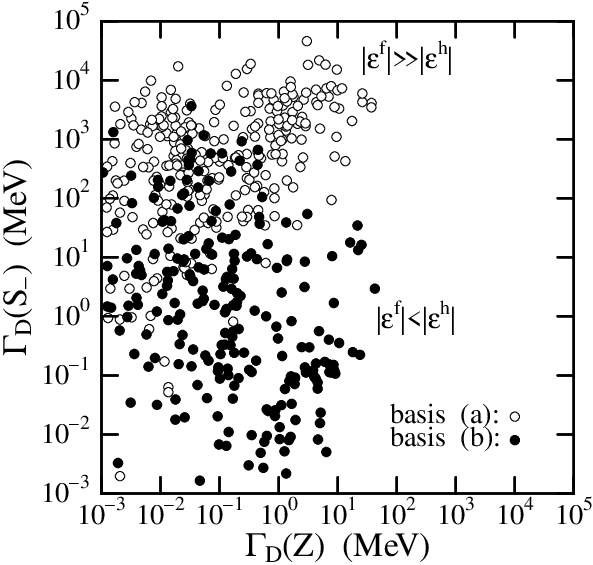
where |ϵf|≡[(ϵ1f)2+(ϵ2f)2+(ϵ3f)2]1/2|\epsilon^{f}|\equiv[(\epsilon^{f}_{1})^{2}+(\epsilon^{f}_{2})^{2}+(\epsilon^{f}_{3})^{2}]^{1/2}. (The actual value is reduced to some extent by the kinematic factor for mD∼mS−m_{D}\sim m_{S^{-}}.) This width ΓD​(S−)\Gamma_{D}(S_{-}) for the decays into the singlet scalar S−S_{-} dominates over the reference width ΓD​(Z)\Gamma_{D}(Z) for the decays into the ZZ boson in Eq. (89) for |ϵf|2≫|ϵh|2|\epsilon^{f}|^{2}\gg|\epsilon^{h}|^{2}, especially in the basis (a) with ϵih→(mdi/mD)​ϵif\epsilon^{h}_{i}\rightarrow(m_{d_{i}}/m_{D})\epsilon^{f}_{i}. As for the DD decays with S+S_{+}, the partial width is simply related to ΓD​(Z)\Gamma_{D}(Z) by Eq. (80) as

ΓD​(S+)≡∑iΓ⁡(D→di​S+)∼(v/vS)2​ΓD​(Z),\displaystyle\Gamma_{D}(S_{+})\equiv\sum_{i}\Gamma(D\rightarrow d_{i}S_{+})\sim(v/v_{S})^{2}\Gamma_{D}(Z), (97)

which amounts to O⁡(10%)O(10\%) of ΓD​(Z)\Gamma_{D}(Z) for vS≈500​GeVv_{S}\approx 500{\rm GeV}. Even this slight enhancement due to ΓD​(S+)\Gamma_{D}(S_{+}) for the DD decays into the scalars HH and S+S_{+} might serve as an experimental signature for the singlet Higgs even if S−S_{-} is absent in the model with one real S≡S+S\equiv S_{+}.

Here, it should be noted that the S−S_{-} coupling may even provide significant contributions to the decays D→di​HD\rightarrow d_{i}H through the HH-S−S_{-} mixing ϵH​S−\epsilon_{HS_{-}} in OϕO_{\phi}. In fact, the dd-DD coupling with the standard Higgs HH (more precisely the mass eigenstate ϕ1≃H\phi_{1}\simeq H with ϵH​S−≪1\epsilon_{HS_{-}}\ll 1) is replaced in Eq. (85) as

Λ𝒟H→Λ𝒟H+ϵH​S−​Λ𝒟S−.\Lambda_{\cal D}^{H}\rightarrow\Lambda_{\cal D}^{H}+\epsilon_{HS_{-}}\Lambda_{\cal D}^{S_{-}}. (98)

Then, instead of Eq. (93) we obtain

ΓD​(H)\displaystyle\Gamma_{D}(H) ∼\displaystyle\sim ΓD​(Z)+ϵH​S−2​ΓD​(S−),\displaystyle\Gamma_{D}(Z)+\epsilon_{HS_{-}}^{2}\Gamma_{D}(S_{-}), (99)

where the interference term between Λ𝒟H\Lambda_{\cal D}^{H} and Λ𝒟S−\Lambda_{\cal D}^{S_{-}} is omitted for simplicity. This enhancement of ΓD​(H)\Gamma_{D}(H) with ϵH​S−​Λ𝒟S−\epsilon_{HS_{-}}\Lambda_{\cal D}^{S_{-}} in Eq. (98) is valid even when the decays D→di​S−D\rightarrow d_{i}S_{-} are forbidden kinematically for mD<mS−+mdim_{D}<m_{S_{-}}+m_{d_{i}}. In the presence of a small but sizable HH-S−S_{-} mixing ϵH​S−∼0.01−0.1\epsilon_{HS_{-}}\sim 0.01-0.1 the singlet quark decays D→di​HD\rightarrow d_{i}H may become the dominant modes, particularly in the basis (a) due to the substantial suppression of D→di​ZD\rightarrow d_{i}Z with |𝒵𝒟​[d†​D]i|2∼(mdi/mD)2​(ϵif)2≲10−4|{\cal Z}_{\cal D}[d^{\dagger}D]_{i}|^{2}\sim(m_{d_{i}}/m_{D})^{2}(\epsilon^{f}_{i})^{2}\lesssim 10^{-4}. Hence, if ΓD​(H)≫ΓD​(Z)\Gamma_{D}(H)\gg\Gamma_{D}(Z) is confirmed experimentally, which is contrary to the usual expectation of Eq. (93), it will provide a distinct evidence for the complex singlet Higgs field SS with the HH-S−S_{-} mixing. The decays D→di​S+D\rightarrow d_{i}S_{+} may also be enhanced substantially as ΓD​(S+)∼ϵS+​S−2​ΓD​(S−)\Gamma_{D}(S_{+})\sim\epsilon_{S_{+}S_{-}}^{2}\Gamma_{D}(S_{-}) via a sizable S+S_{+}-S−S_{-} mixing ϵS+​S−\epsilon_{S_{+}S_{-}}.

We present in the following the detailed estimates on the widths of the relevant decay modes, where the constraints on the dd-DD mixing from the Δ​F=2\Delta F=2 meson mixings and the diagonal ZZ-boson couplings are checked to be satisfied according to the numerical calculations performed in Sec. III.

Refer to caption
Figure 5: RD​(W/Z)≡ΓD​(W)/ΓD​(Z)R_{D}(W/Z)\equiv\Gamma_{D}(W)/\Gamma_{D}(Z) versus mDm_{D} is shown for the bases (a) (□\Box) and (b) (■\blacksquare). RD​(H/Z)≡ΓD​(H)/ΓD​(Z)R_{D}(H/Z)\equiv\Gamma_{D}(H)/\Gamma_{D}(Z) versus mDm_{D} is also shown for the bases (a) (△\vartriangle) and (b) (▲\blacktriangle). Here, vS=500​GeVv_{S}=500{\rm GeV}, and the Higgs scalar mixing is assumed to be absent (Oϕ=𝟏O_{\phi}={\bf 1}).

We suitably denote the ratios of the relevant widths to the reference width as

RD​(X/Z)≡ΓD​(X)ΓD​(Z),\displaystyle R_{D}(X/Z)\equiv\frac{\Gamma_{D}(X)}{\Gamma_{D}(Z)}, (100)

where X=W,H,S+,S−X=W,H,S_{+},S_{-}. For the usual decay modes D→ui​WD\rightarrow u_{i}W, D→di​ZD\rightarrow d_{i}Z and D→di​HD\rightarrow d_{i}H, scatter plots of RD​(W/Z)R_{D}(W/Z) (□\Box, ■\blacksquare) and RD​(H/Z)R_{D}(H/Z) (△\vartriangle, ▲\blacktriangle) versus the singlet quark mass mDm_{D} are shown in Fig. 5 for the bases (a) (□\Box, △\vartriangle) and (b) (■\blacksquare, ▲\blacktriangle). Here, vS=500​GeVv_{S}=500{\rm GeV}, and the Higgs scalar mixing is assumed to be absent (Oϕ=𝟏O_{\phi}={\bf 1}). Similar results are obtained for the bases (a) and (b) since these bases are equivalently related to each other by the unitary transformation, as discussed in Sec. II. Note here that larger values may be obtained for the singlet quark mass mDm_{D} with a given singlet Higgs VEV vSv_{S} in the basis (a) (□\Box, △\vartriangle), which is due to the significant contribution of the qq-QQ mixing term Δq​Q=fQ+​vS/2\Delta_{qQ}=f_{Q}^{+}v_{S}/{\sqrt{2}} for |ϵf|∼1|\epsilon^{f}|\sim 1. The lower boundary curve for RD​(W/Z)R_{D}(W/Z) reflects the kinematic factor of the dominant top contribution D→t​WD\rightarrow tW with |𝒱​[u†​D]3|2≫|𝒱​[u†​D]1,2|2|{\cal V}[u^{\dagger}D]_{3}|^{2}\gg|{\cal V}[u^{\dagger}D]_{1,2}|^{2}. In this case the singlet DD quark mixes mainly with the bb quark as |(ϵdL)3|2≫|(ϵdL)1,2|2|(\epsilon_{d_{\rm L}})_{3}|^{2}\gg|(\epsilon_{d_{\rm L}})_{1,2}|^{2}. On the other hand, in the case that the top contribution is negligible with |𝒱​[u†​D]3|2≪|𝒱​[u†​D]1,2|2|{\cal V}[u^{\dagger}D]_{3}|^{2}\ll|{\cal V}[u^{\dagger}D]_{1,2}|^{2}, the asymptotic value RD​(W/Z)=2R_{D}(W/Z)=2 is almost saturated for mD≳300​GeVm_{D}\gtrsim 300{\rm GeV}. We also see that RD​(H/Z)R_{D}(H/Z) approaches the asymptotic value RD​(H/Z)=1R_{D}(H/Z)=1 showing the kinematic dependence on mDm_{D}. These results really confirm the usual expectation in Eqs. (92) and (93). It should, however, be remarked that as shown in Eq. (99), the DD decays with the standard Higgs HH may be enhanced substantially as RD​(H/Z)≫1R_{D}(H/Z)\gg 1 due to the singlet Higgs coupling Λ𝒟S−\Lambda_{\cal D}^{S_{-}} via the HH-S−S_{-} mixing.

The reference width ΓD​(Z)\Gamma_{D}(Z) versus the magnitude of the left-handed dd-DD mixing |ϵh||\epsilon^{h}|, as given in Eq. (89), is shown in Fig. 6. Here, the marks ∘\circ and ∙\bullet denote the estimates in the bases (a) and (b), respectively, and ϵih=(mqi/mD)​ϵif\epsilon^{h}_{i}=(m_{q_{i}}/m_{D})\epsilon^{f}_{i} as Eq. (43) is adopted in the basis (a) though ϵih=0\epsilon^{h}_{i}=0 formally. This plot of ΓD​(Z)\Gamma_{D}(Z) spreads according to the variation of mD∼100​GeV−1​TeVm_{D}\sim 100{\rm GeV}-1{\rm TeV} due to the fact that ΓD​(Z)\Gamma_{D}(Z) is almost proportional to mD3m_{D}^{3}.

Refer to caption
Figure 6: ΓD​(Z)\Gamma_{D}(Z) versus |ϵh||\epsilon^{h}| in the bases (a) (∘\circ) and (b) (∙\bullet). Here, ϵih=(mqi/mD)​ϵif\epsilon^{h}_{i}=(m_{q_{i}}/m_{D})\epsilon^{f}_{i} as Eq. (43) is adopted in the basis (a) though ϵih=0\epsilon^{h}_{i}=0 formally.
Refer to caption
Figure 7: ΓD​(Z)\Gamma_{D}(Z) and ΓD​(S−)\Gamma_{D}(S_{-}) are compared in the bases (a) (∘\circ) and (b) (∙\bullet).
Refer to caption
Figure 8: RD​(H/Z)≡ΓD​(H)/ΓD​(Z)R_{D}(H/Z)\equiv\Gamma_{D}(H)/\Gamma_{D}(Z) versus |ϵf|/|ϵh||\epsilon^{f}|/|\epsilon^{h}| is shown for the bases (a) (△\vartriangle) and (b) (▲\blacktriangle), where ϵH​S−=0.1\epsilon_{HS_{-}}=0.1 is taken typically for the HH-S−S_{-} mixing.

The decay widths ΓD​(Z)\Gamma_{D}(Z) and ΓD​(S−)\Gamma_{D}(S_{-}) for the significant modes are compared in Fig. 7. According to Eqs. (89) and (96), by measuring these decay widths we can estimate the magnitudes of dd-DD mixings, |ϵh||\epsilon^{h}| from the hdh_{d} coupling and |ϵf||\epsilon^{f}| from the fDf_{D} and fD′f_{D}^{\prime} couplings. Specifically, ΓD​(S−)≫ΓD​(Z)\Gamma_{D}(S_{-})\gg\Gamma_{D}(Z) for |ϵf|≫|ϵh||\epsilon^{f}|\gg|\epsilon^{h}| as in the basis (a) (∘\circ), while ΓD​(S−)≲ΓD​(Z)\Gamma_{D}(S_{-})\lesssim\Gamma_{D}(Z) for |ϵf|≲|ϵh||\epsilon^{f}|\lesssim|\epsilon^{h}| as in the basis (b) (∙\bullet). The decay width ΓD​(H)\Gamma_{D}(H) with the standard Higgs HH is also relevant to measure the relative significance of |ϵh||\epsilon^{h}| versus |ϵf||\epsilon^{f}| according to Eq. (99) with the sizable HH-S−S_{-} mixing. This is useful even if the decays D→di​S−D\rightarrow d_{i}S_{-} are kinematically forbidden for mS−>mD+mdim_{S-}>m_{D}+m_{d_{i}}. A plot of RD​(H/Z)R_{D}(H/Z) versus |ϵf|/|ϵh||\epsilon^{f}|/|\epsilon^{h}| is shown in Fig. 8 for the bases (a) (△\vartriangle) and (b) (▲\blacktriangle), where ϵH​S−=0.1\epsilon_{HS_{-}}=0.1 is taken typically for the HH-S−S_{-} mixing. In the region of |ϵf|/|ϵh|≫1|\epsilon^{f}|/|\epsilon^{h}|\gg 1, the contribution of the singlet Higgs coupling Λ𝒟S−\Lambda_{\cal D}^{S_{-}} dominates as ΓD​(H)∼ϵH​S−2​ΓD​(S−)≫ΓD​(Z)\Gamma_{D}(H)\sim\epsilon_{HS^{-}}^{2}\Gamma_{D}(S_{-})\gg\Gamma_{D}(Z). On the other hand, in the region of |ϵf|/|ϵh|≲1|\epsilon^{f}|/|\epsilon^{h}|\lesssim 1 we have ΓD​(H)∼ΓD​(Z)\Gamma_{D}(H)\sim\Gamma_{D}(Z) as usually expected.

In these plots of Figs. 5, 6, 7 and 8, the regions for the bases (a) and (b) overlap as expected, but they are not identical. This is because the actual parameter ranges are somewhat different for the bases (a) and (b); although the parameter ranges have been taken apparently in the same way for these bases in the numerical calculations, except that hq=𝟎h_{q}={\bf 0} in the basis (a), they are not mapped identically to each other by the unitary transformation between the bases (a) and (b). Specifically, in the basis (a) we have a significant constraint |ϵh|/|ϵf|≲mb/mD∼0.01|\epsilon^{h}|/|\epsilon^{f}|\lesssim m_{b}/m_{D}\sim 0.01 from the relation ϵih∼(mdi/mD)​ϵif\epsilon^{h}_{i}\sim(m_{d_{i}}/m_{D})\epsilon^{f}_{i}, implying |ϵh|≲0.01|\epsilon^{h}|\lesssim 0.01 as long as |ϵf|≲1|\epsilon^{f}|\lesssim 1. This is explicitly seen in Figs. 6 and 8. We also note that the plot for the basis (a) in Fig. 8 spreads significantly. This is in some sense an artifact due to the definition of the dd-DD mixing parameters ϵif\epsilon^{f}_{i} in terms of fD+≡fD+fD′f_{D}^{+}\equiv f_{D}+f^{\prime}_{D} for the basis (a). The singlet S−S_{-} coupling Λ𝒟S−\Lambda_{\cal D}^{S_{-}} is rather given by fD−≡i⁡(fD−fD′)f_{D}^{-}\equiv i(f_{D}-f^{\prime}_{D}). The spread in the plot for the basis (a) really reflects the partial cancellation between fDf_{D} and fD′f^{\prime}_{D} for the Λ𝒟S−\Lambda_{\cal D}^{S_{-}} coupling. On the other hand, for the basis (b) the parameters ϵif\epsilon^{f}_{i} are defined suitably with fD−=2​i​fDf_{D}^{-}=2if_{D} (fD=−fD′f_{D}=-f^{\prime}_{D} for fD+=𝟎f_{D}^{+}={\bf 0}). Hence, the plot for the basis (b) almost lies on a curve up to the small fluctuation due to the kinematic factor, which gives the boundary of the plot for the basis (a). This boundary really corresponds to the extreme case fD≈−fD′f_{D}\approx-f^{\prime}_{D} for |fD−|≈2​|fD||f_{D}^{-}|\approx 2|f_{D}| in the basis (a).

As seen so far, the singlet DD quark decays present us important insights on the dd-DD mixing effects for the flavor-changing processes. Especially, if it is observed that ΓD​(S−)≫ΓD​(Z)\Gamma_{D}(S_{-})\gg\Gamma_{D}(Z), we find that the singlet Higgs scalar interactions dominate over the ZZ-boson interactions. For example, suppose that the current experimental bound for the BdB_{d}-B¯d{\bar{B}_{d}} mixing [38] is almost saturated with (ϵ1f​ϵ3f)12∼0.2(\epsilon^{f}_{1}\epsilon^{f}_{3})^{\frac{1}{2}}\sim 0.2 for mS−∼300​GeVm_{S_{-}}\sim 300{\rm GeV} in the basis (a) as shown in Eq. (III), which implies |ϵf|≳2×0.2≫|ϵh||\epsilon^{f}|\gtrsim{\sqrt{2}}\times 0.2\gg|\epsilon^{h}|. Then, we expect ΓD​(S−)∼1​GeV−10​GeV≫ΓD​(Z)\Gamma_{D}(S_{-})\sim 1{\rm GeV}-10{\rm GeV}\gg\Gamma_{D}(Z) for mD∼500​GeV−1​TeVm_{D}\sim 500{\rm GeV}-1{\rm TeV}, as seen in Eq. (96) and Fig. 7. Contrarily, if ΓD​(S−)≲1​MeV\Gamma_{D}(S_{-})\lesssim 1{\rm MeV} for mD≳500​GeVm_{D}\gtrsim 500{\rm GeV}, which implies |ϵf|≲0.01|\epsilon^{f}|\lesssim 0.01, the scalar FCNC’s do not provide significant contributions to the Δ​F=2\Delta F=2 meson mixings. As for the DD decays with the ZZ boson, if there is a significant left-handed dd-DD mixing as |ϵh|∼0.03|\epsilon^{h}|\sim 0.03 in the basis (b), we expect ΓD​(Z)∼10​MeV−100​MeV\Gamma_{D}(Z)\sim 10{\rm MeV}-100{\rm MeV} for mD∼500​GeV−1​TeVm_{D}\sim 500{\rm GeV}-1{\rm TeV} in Eq. (89). In this case, the bound for the BdB_{d}-B¯d{\bar{B}_{d}} mixing may be saturated by the ZZ-mediated FCNC with (ϵ1h​ϵ3h)12∼0.03(\epsilon^{h}_{1}\epsilon^{h}_{3})^{\frac{1}{2}}\sim 0.03, as shown in Eq. (III). On the other hand, if ΓD​(Z)≲0.01​MeV\Gamma_{D}(Z)\lesssim 0.01{\rm MeV} for mD≳500​GeVm_{D}\gtrsim 500{\rm GeV}, which implies |ϵh|≲0.001|\epsilon^{h}|\lesssim 0.001 (see Fig. 6), the effects of the ZZ-mediated FCNC’s are negligible in the Δ​F=2\Delta F=2 meson mixings.

IV.2 Higgs particle decays

We next survey the decays of the Higgs particles HH, S+S_{+} and S−S_{-}, or more precisely the mass eigenstates ϕ1\phi_{1}, ϕ2\phi_{2}, ϕ3\phi_{3} with the mixing matrix OϕO_{\phi}.

The standard Higgs HH is probably lighter than the singlet quarks QQ (mQ>mH≈120​GeVm_{Q}>m_{H}\approx 120{\rm GeV}) so that its decays involving the singlet quarks are forbidden kinematically. It should also be noted that the qq-QQ mixing effect on the HH coupling with the ordinary quarks appears merely at the second order related to the modification of the ZZ-boson coupling, as seen in Eq. (39). Hence, the Higgs particle HH will decay essentially in the same way as the standard model unless the HH-S−S_{-} mixing is so large as to provide significant effects.

The singlet Higgs particles S±S_{\pm} will be produced significantly by gluon fusion via a loop of singlet quark QQ coupled to S±S_{\pm} with the strength ∼|λQ±|∼mQ/vS∼1\sim|\lambda_{Q}^{\pm}|\sim m_{Q}/v_{S}\sim 1. The production rates of S±S_{\pm} will be comparable to that of the standard Higgs HH unless S±S_{\pm} are substantially heavier than HH. If mS±<mQm_{S_{\pm}}<m_{Q}, the singlet quark decays Q→qi​S±Q\rightarrow q_{i}S_{\pm} also produce S±S_{\pm}, as discussed so far. It should be remarked that some indirect indication for the presence of S−S_{-} may be obtained via the HH-S−S_{-} mixing, specifically in the case of ΓQ​(H)≫ΓQ​(Z)\Gamma_{Q}(H)\gg\Gamma_{Q}(Z) for the singlet quark decays Q→q​HQ\rightarrow qH.

In the case of mS±<mQm_{S_{\pm}}<m_{Q}, the singlet Higgs particles S±S_{\pm} decay predominantly into the ordinary quarks through the scalar interactions in Eqs. (40), (41) and (42) at the second order of the qq-QQ mixing:

S±→qi​q¯j.\displaystyle S_{\pm}\rightarrow q_{i}{\bar{q}}_{j}. (101)

The decay widths are estimated particularly for S−S_{-} in comparison with that of the standard Higgs HH as

Γ⁡(S−→qi​q¯j)Γ⁡(H→b​b¯)\displaystyle\frac{\Gamma(S_{-}\rightarrow q_{i}{\bar{q}}_{j})}{\Gamma(H\rightarrow b{\bar{b}})} ∼\displaystyle\sim mS−​(|Λ𝒬S−​[qc​q]i​j|2+|Λ𝒬S−​[qc​q]j​i|2)mH​|Λ𝒬H​[qc​q]33|2\displaystyle\frac{m_{S_{-}}(|\Lambda_{\cal Q}^{S_{-}}[q^{c}q]_{ij}|^{2}+|\Lambda_{\cal Q}^{S_{-}}[q^{c}q]_{ji}|^{2})}{m_{H}|\Lambda_{\cal Q}^{H}[q^{c}q]_{33}|^{2}} (102)
∼\displaystyle\sim [(mS−/mH)​(mQ/vS)2/(mb/v)2]\displaystyle[(m_{S_{-}}/m_{H})(m_{Q}/v_{S})^{2}/(m_{b}/v)^{2}]
×[(ϵif)2​(ϵjh)2+(ϵjf)2​(ϵih)2],\displaystyle\times[(\epsilon^{f}_{i})^{2}(\epsilon^{h}_{j})^{2}+(\epsilon^{f}_{j})^{2}(\epsilon^{h}_{i})^{2}],

where ϵjh→(mqj/mQ)​ϵjf\epsilon^{h}_{j}\rightarrow(m_{q_{j}}/m_{Q})\epsilon^{f}_{j} in the basis (a). We estimate, for instance, Γ⁡(S−→b​b¯)/Γ⁡(H→b​b¯)∼[10​(ϵ3f​ϵ3h)12]4\Gamma(S_{-}\rightarrow b{\bar{b}})/\Gamma(H\rightarrow b{\bar{b}})\sim[10(\epsilon^{f}_{3}\epsilon^{h}_{3})^{\frac{1}{2}}]^{4} for mS−/mH∼3m_{S_{-}}/m_{H}\sim 3, mD/vS∼1m_{D}/v_{S}\sim 1 and mb/v≃1/60m_{b}/v\simeq 1/60, which may amount to O⁡(1)O(1) for the large bb-DD mixing as ϵ3f∼1\epsilon^{f}_{3}\sim 1 and ϵ3h∼(mb/mD)​ϵ3f∼0.01\epsilon^{h}_{3}\sim(m_{b}/m_{D})\epsilon^{f}_{3}\sim 0.01. The flavor-changing decays such as S−→b​s¯S_{-}\rightarrow b{\bar{s}} as well as the flavor-diagonal ones may have significant fractions. This is distinct from the standard Higgs HH, presenting a promising signature of the singlet Higgs S−S_{-}. In fact, we estimate

Γ⁡(S−→b​d¯j)Γ⁡(S−→b​b¯)\displaystyle\frac{\Gamma(S_{-}\rightarrow b{\bar{d}}_{j})}{\Gamma(S_{-}\rightarrow b{\bar{b}})} ∼\displaystyle\sim (ϵjf/ϵ3f)2+(ϵjh/ϵ3h)2,\displaystyle(\epsilon^{f}_{j}/\epsilon^{f}_{3})^{2}+(\epsilon^{h}_{j}/\epsilon^{h}_{3})^{2}, (103)

depending on the flavor structure of the dd-DD mixing. If the singlet UU quarks are present with a large tt-UU mixing, the decays S−→t​t¯,t​u¯i,ui​t¯S_{-}\rightarrow t{\bar{t}},t{\bar{u}}_{i},u_{i}{\bar{t}} involving the top quark may be observed with significant fractions.

In this way, the decays of the singlet Higgs S−S_{-} into the ordinary quarks are determined in terms of the qq-QQ mixing parameters with close connection to the flavor-changing processes such as the Δ​F=2\Delta F=2 meson mixings. As for the the singlet Higgs S+S_{+}, its coupling is given in Eq. (40) by the ZZ-boson coupling at the second order of qq-QQ mixing with further suppression by the ordinary quark mass. These arguments on the S±S_{\pm} couplings with the ordinary quarks generally suggest that

ΓH≳ΓS−≫ΓS+​(mS±<mQ,Oϕ≈𝟏).\displaystyle\Gamma_{H}\gtrsim\Gamma_{S-}\gg\Gamma_{S_{+}}(m_{S_{\pm}}<m_{Q},O_{\phi}\approx{\bf 1}). (104)

for the decay rates of the Higgs particles if the Higgs mixing is negligibly small. It is, however, possible that the large Higgs mixing, in cooperation with the qq-QQ mixing, affects significantly the decays of HH and S±S_{\pm}. (See also Ref. [42] for investigations of extended Higgs models at the LHC.) Therefore, the observations of the Higgs particle decays present important information on the Higgs mixing and qq-QQ mixing.

In the case of mS±>mQm_{S_{\pm}}>m_{Q}, the singlet quark decays Q→q​S±Q\rightarrow qS_{\pm} are forbidden kinematically. Even in such a case the singlet Higgs S±S_{\pm} will be produced significantly by the gluon fusion via the singlet quark loop. Then, they decay predominantly involving the singlet quarks as

S±→Q​q¯,Q¯​q,Q​Q¯.\displaystyle S_{\pm}\rightarrow Q{\bar{q}},{\bar{Q}}q,Q{\bar{Q}}. (105)

The decay widths are estimated in terms of the scalar couplings Λ𝒬S±\Lambda_{\cal Q}^{S_{\pm}} in Eq. (II.2). In particular, if mS±>2​mQm_{S_{\pm}}>2m_{Q} we have

Γ⁡(S±→Q​Q¯)∼(mQ/vS)2​mS±16​π≳10​G​e​V≫ΓH\displaystyle\Gamma(S_{\pm}\rightarrow Q{\bar{Q}})\sim\frac{(m_{Q}/v_{S})^{2}m_{S_{\pm}}}{16\pi}\gtrsim 10{\rm GeV}\gg\Gamma_{H} (106)

with Br⁡(S±→Q​Q¯)≈1{\rm Br}(S_{\pm}\rightarrow Q{\bar{Q}})\approx 1 for mS±≳500​GeVm_{S_{\pm}}\gtrsim 500{\rm GeV} and |λQ±|∼mQ/vS∼1|\lambda_{Q}^{\pm}|\sim m_{Q}/v_{S}\sim 1.

V Summary

The singlet quarks in cooperation with the single Higgs field may provide various interesting effects in particle physics and cosmology through the mixing with the ordinary quarks (qq-QQ mixing). It is hence worth considering their phenomenological implications toward the discovery of them at the LHC. In this study we have investigated the flavor-changing interactions in the model with singlet quarks and singlet Higgs, which are induced by the qq-QQ mixing. While the gauge interactions have been investigated extensively in the literature, we have rather noted here that the scalar interactions mediated by the singlet Higg may provide significant effects in some cases. This possibility has not been paid so much attention before in the models with singlet quarks. We have considered the effects of the gauge and scalar interactions in the Δ​F=2\Delta F=2 mixings of the neutral mesons to show the currently allowed range of the qq-QQ mixing. Then, we have investigated the decays of the singlet quarks and Higgs particles as the new physics around the electroweak scale to the TeV scale, which is accessible to the LHC. Especially, the right-handed qq-QQ mixing may be tolerably large without contradicting the current bounds on the flavor-changing processes, since it is not involved directly in the electroweak gauge interactions. If this is the case, the scalar coupling by the singlet Higgs, and possibly through the Higgs mixing, provides distinct signatures for the decays of the singlet quarks and Higgs particles, which should be compared with the conventionally expected ones via the gauge and standard Higgs couplings. We expect that observations of the singlet quarks and Higgs particles will present us important insights on the qq-QQ mixing and Higgs mixing.

Acknowledgements.
We would like to thank M. Senami for valuable discussions.

Appendix A Relations among the gauge and scalar couplings

We here derive the suitable relations among the gauge and scalar couplings.

The full mixing matrix for the left-handed WW-boson coupling is given by

𝒱\displaystyle{\cal V} =\displaystyle= 𝒱𝒰L†​(V0𝟎𝟎𝟎)​𝒱𝒟L\displaystyle{\cal V}_{{\cal U}_{\rm L}}^{\dagger}\left(\begin{array}[]{cc}V_{0}&{\bf 0}\\ {\bf 0}&{\bf 0}\end{array}\right){\cal V}_{{\cal D}_{\rm L}}
=\displaystyle= (VuL†​V0​VdLVuL†​V0​ϵdLϵuL†​V0​VdLϵuL†​V0​ϵdL).\displaystyle\left(\begin{array}[]{cc}V_{u_{\rm L}}^{\dagger}V_{0}V_{d_{\rm L}}&V_{u_{\rm L}}^{\dagger}V_{0}\epsilon_{d_{\rm L}}\\ \epsilon_{u_{\rm L}}^{\dagger}V_{0}V_{d_{\rm L}}&\epsilon_{u_{\rm L}}^{\dagger}V_{0}\epsilon_{d_{\rm L}}\end{array}\right).

Then, we obtain from the off-diagonal blocks

𝒱⁡[u†​D]\displaystyle{\cal V}[u^{\dagger}D] =\displaystyle= VuL†​V0​ϵdL≃V​VdL†​ϵdL,\displaystyle V_{u_{\rm L}}^{\dagger}V_{0}\epsilon_{d_{\rm L}}\simeq VV_{d_{\rm L}}^{\dagger}\epsilon_{d_{\rm L}}, (113)
𝒱⁡[U†​d]\displaystyle{\cal V}[U^{\dagger}d] =\displaystyle= ϵuL†​V0​VdL≃ϵuL†​VuL​V,\displaystyle\epsilon_{u_{\rm L}}^{\dagger}V_{0}V_{d_{\rm L}}\simeq\epsilon_{u_{\rm L}}^{\dagger}V_{u_{\rm L}}V, (114)

where the approximate unitarity VqL​VqL†≃𝟏V_{q_{\rm L}}V_{q_{\rm L}}^{\dagger}\simeq{\bf 1} is considered up to the second order of the small qq-QQ mixing. By applying Eq. (74) for the ZZ-boson coupling to Eqs. (113) and (114), we obtain Eqs. (75) and (76).

The left-handed ZZ-boson coupling is given originally in the electroweak basis (q0,Q0)(q_{0},Q_{0}) as

𝒵𝒬(0)=(𝟏𝟎𝟎𝟎)−a⁡(𝟏𝟎𝟎𝟏),\displaystyle{\cal Z}_{\cal Q}^{(0)}=\left(\begin{array}[]{cc}{\bf 1}&{\bf 0}\\ {\bf 0}&{\bf 0}\end{array}\right)-a\left(\begin{array}[]{cc}{\bf 1}&{\bf 0}\\ {\bf 0}&{\bf 1}\end{array}\right),

where a=sin2⁡θW​Qem​(𝒬)/I3​(q0)a=\sin^{2}\theta_{W}Q_{\rm em}({\cal Q})/I_{3}(q_{0}), and the division by I3(q0)=±1/2I_{3}(q_{0})=\pm 1/2 is for convenience of notation. It is transformed in the basis of mass eigenstates (q,Q)(q,Q) as

𝒵𝒬\displaystyle{\cal Z}_{\cal Q} =\displaystyle= 𝒱𝒬L†​𝒵𝒬(0)​𝒱𝒬L\displaystyle{\cal V}_{{\cal Q}_{\rm L}}^{\dagger}{\cal Z}_{\cal Q}^{(0)}{\cal V}_{{\cal Q}_{\rm L}}
=\displaystyle= 𝒱𝒬L†​(𝟏𝟎𝟎𝟎)​𝒱𝒬L−a​(𝟏𝟎𝟎𝟏).\displaystyle{\cal V}_{{\cal Q}_{\rm L}}^{\dagger}\left(\begin{array}[]{cc}{\bf 1}&{\bf 0}\\ {\bf 0}&{\bf 0}\end{array}\right){\cal V}_{{\cal Q}_{\rm L}}-a\left(\begin{array}[]{cc}{\bf 1}&{\bf 0}\\ {\bf 0}&{\bf 1}\end{array}\right).

The modification of the ZZ-boson coupling due to the qq-QQ mixing is calculated from Eqs. (A) and (A) as

Δ​𝒵𝒬\displaystyle\Delta{\cal Z}_{\cal Q} =\displaystyle= 𝒵𝒬−𝒵𝒬(0)\displaystyle{\cal Z}_{\cal Q}-{\cal Z}_{\cal Q}^{(0)}
=\displaystyle= 𝒱𝒬L†​(𝟏𝟎𝟎𝟎)​𝒱𝒬L−(𝟏𝟎𝟎𝟎)\displaystyle{\cal V}_{{\cal Q}_{\rm L}}^{\dagger}\left(\begin{array}[]{cc}{\bf 1}&{\bf 0}\\ {\bf 0}&{\bf 0}\end{array}\right){\cal V}_{{\cal Q}_{\rm L}}-\left(\begin{array}[]{cc}{\bf 1}&{\bf 0}\\ {\bf 0}&{\bf 0}\end{array}\right)
=\displaystyle= (−ϵqL′​ϵqL′⁣†VqL†​ϵqLϵqL†​VqLϵqL†​ϵqL).\displaystyle\left(\begin{array}[]{cc}-\epsilon_{q_{\rm L}}^{\prime}\epsilon_{q_{\rm L}}^{\prime\dagger}&V_{q_{\rm L}}^{\dagger}\epsilon_{q_{\rm L}}\\ \epsilon_{q_{\rm L}}^{\dagger}V_{q_{\rm L}}&\epsilon_{q_{\rm L}}^{\dagger}\epsilon_{q_{\rm L}}\end{array}\right).

Here, we have considered the relation VqL†​VqL−𝟏=−ϵqL′​ϵqL′⁣†V_{q_{\rm L}}^{\dagger}V_{q_{\rm L}}-{\bf 1}=-\epsilon_{q_{\rm L}}^{\prime}\epsilon_{q_{\rm L}}^{\prime\dagger} from the unitarity of 𝒱𝒬L{\cal V}_{{\cal Q}_{\rm L}} to obtain Eq. (26) for the upper diagonal block Δ​𝒵𝒬​[q†​q]\Delta{\cal Z}_{\cal Q}[q^{\dagger}q] in Δ​𝒵𝒬\Delta{\cal Z}_{\cal Q}. We also obtain the ZZ boson qq-QQ couplings in Eq. (74) from the off-diagonal blocks in Eqs. (A) and (A) as

𝒵𝒬​[q†​Q]=Δ​𝒵𝒬​[q†​Q]=VqL†​ϵqL=(𝒵𝒬​[Q†​q])†.\displaystyle{\cal Z}_{\cal Q}[q^{\dagger}Q]=\Delta{\cal Z}_{\cal Q}[q^{\dagger}Q]=V_{q_{\rm L}}^{\dagger}\epsilon_{q_{\rm L}}=({\cal Z}_{\cal Q}[Q^{\dagger}q])^{\dagger}. (133)

We note the relation from Eq. (A) as

𝒱𝒬L†​(𝟏𝟎𝟎𝟎)​𝒱𝒬L=Δ​𝒵𝒬+(𝟏𝟎𝟎𝟎).\displaystyle{\cal V}_{{\cal Q}_{\rm L}}^{\dagger}\left(\begin{array}[]{cc}{\bf 1}&{\bf 0}\\ {\bf 0}&{\bf 0}\end{array}\right){\cal V}_{{\cal Q}_{\rm L}}=\Delta{\cal Z}_{\cal Q}+\left(\begin{array}[]{cc}{\bf 1}&{\bf 0}\\ {\bf 0}&{\bf 0}\end{array}\right).

By taking the difference between this relation and that for the unit matrix

𝒱𝒬L†​(𝟏𝟎𝟎𝟏)​𝒱𝒬L=(𝟏𝟎𝟎𝟏),\displaystyle{\cal V}_{{\cal Q}_{\rm L}}^{\dagger}\left(\begin{array}[]{cc}{\bf 1}&{\bf 0}\\ {\bf 0}&{\bf 1}\end{array}\right){\cal V}_{{\cal Q}_{\rm L}}=\left(\begin{array}[]{cc}{\bf 1}&{\bf 0}\\ {\bf 0}&{\bf 1}\end{array}\right),

we obtain another relation

𝒱𝒬L†​(𝟎𝟎𝟎𝟏)​𝒱𝒬L=−Δ​𝒵𝒬+(𝟎𝟎𝟎𝟏).\displaystyle{\cal V}_{{\cal Q}_{\rm L}}^{\dagger}\left(\begin{array}[]{cc}{\bf 0}&{\bf 0}\\ {\bf 0}&{\bf 1}\end{array}\right){\cal V}_{{\cal Q}_{\rm L}}=-\Delta{\cal Z}_{\cal Q}+\left(\begin{array}[]{cc}{\bf 0}&{\bf 0}\\ {\bf 0}&{\bf 1}\end{array}\right).

By using Eq. (A), we calculate

𝒱𝒬R†​ℳ𝒬​(𝟏𝟎𝟎𝟎)​𝒱𝒬L\displaystyle{\cal V}_{{\cal Q}_{\rm R}}^{\dagger}{\cal M}_{\cal Q}\left(\begin{array}[]{cc}{\bf 1}&{\bf 0}\\ {\bf 0}&{\bf 0}\end{array}\right){\cal V}_{{\cal Q}_{\rm L}} =\displaystyle= ℳ¯𝒬​𝒱𝒬L†​(𝟏𝟎𝟎𝟎)​𝒱𝒬L\displaystyle{\bar{\cal M}}_{\cal Q}{\cal V}_{{\cal Q}_{\rm L}}^{\dagger}\left(\begin{array}[]{cc}{\bf 1}&{\bf 0}\\ {\bf 0}&{\bf 0}\end{array}\right){\cal V}_{{\cal Q}_{\rm L}}
=\displaystyle= ℳ¯𝒬​Δ​𝒵𝒬+(M¯q𝟎𝟎𝟎).\displaystyle{\bar{\cal M}}_{\cal Q}\Delta{\cal Z}_{\cal Q}+\left(\begin{array}[]{cc}{\bar{M}}_{q}&{\bf 0}\\ {\bf 0}&{\bf 0}\end{array}\right).

On the other hand, by considering Eq. (6) for MqM_{q} and Δq​Q′\Delta_{qQ}^{\prime} in ℳ𝒬{\cal M}_{\cal Q} we obtain Λ𝒬H\Lambda_{\cal Q}^{H} in Eq. (II.2) as

𝒱𝒬R†​ℳ𝒬​(𝟏𝟎𝟎𝟎)​𝒱𝒬L\displaystyle{\cal V}_{{\cal Q}_{\rm R}}^{\dagger}{\cal M}_{\cal Q}\left(\begin{array}[]{cc}{\bf 1}&{\bf 0}\\ {\bf 0}&{\bf 0}\end{array}\right){\cal V}_{{\cal Q}_{\rm L}} =\displaystyle= v2​𝒱𝒬R†​(λq𝟎hq𝟎)​𝒱𝒬L.\displaystyle\frac{v}{\sqrt{2}}{\cal V}_{{\cal Q}_{\rm R}}^{\dagger}\left(\begin{array}[]{cc}\lambda_{q}&{\bf 0}\\ h_{q}&{\bf 0}\end{array}\right){\cal V}_{{\cal Q}_{\rm L}}.

Comparison of Eqs. () and () establishes the relation between the ZZ-boson coupling and the standard Higgs HH coupling,

Λ𝒬H=(ℳ¯𝒬/v)​Δ​𝒵𝒬+(M¯q/v𝟎𝟎𝟎).\displaystyle\Lambda_{\cal Q}^{H}=({\bar{\cal M}}_{\cal Q}/v)\Delta{\cal Z}_{\cal Q}+\left(\begin{array}[]{cc}{\bar{M}}_{q}/v&{\bf 0}\\ {\bf 0}&{\bf 0}\end{array}\right).

Specifically, Eq. (39) is obtained from the upper diagonal block, and Eqs. (77) and (78) from the off-diagonal blocks with 𝒵𝒬​[q†​Q]=Δ​𝒵𝒬​[q†​Q]{\cal Z}_{\cal Q}[q^{\dagger}Q]=\Delta{\cal Z}_{\cal Q}[q^{\dagger}Q].

Similarly, we obtain the relation between the ZZ-boson coupling and the singlet Higgs S+S_{+} coupling as follows. By using Eq. (A), we calculate

𝒱𝒬R†​ℳ𝒬​(𝟎𝟎𝟎𝟏)​𝒱𝒬L\displaystyle{\cal V}_{{\cal Q}_{\rm R}}^{\dagger}{\cal M}_{\cal Q}\left(\begin{array}[]{cc}{\bf 0}&{\bf 0}\\ {\bf 0}&{\bf 1}\end{array}\right){\cal V}_{{\cal Q}_{\rm L}} =\displaystyle= ℳ¯𝒬​𝒱𝒬L†​(𝟎𝟎𝟎𝟏)​𝒱𝒬L\displaystyle{\bar{\cal M}}_{\cal Q}{\cal V}_{{\cal Q}_{\rm L}}^{\dagger}\left(\begin{array}[]{cc}{\bf 0}&{\bf 0}\\ {\bf 0}&{\bf 1}\end{array}\right){\cal V}_{{\cal Q}_{\rm L}}
=\displaystyle= −ℳ¯𝒬​Δ​𝒵𝒬+(𝟎𝟎𝟎M¯Q).\displaystyle-{\bar{\cal M}}_{\cal Q}\Delta{\cal Z}_{\cal Q}+\left(\begin{array}[]{cc}{\bf 0}&{\bf 0}\\ {\bf 0}&{\bar{M}}_{Q}\end{array}\right).

On the other hand, by considering Eq. (7) for Δq​Q\Delta_{qQ} and MQM_{Q} in ℳ𝒬{\cal M}_{\cal Q} we obtain Λ𝒬S+\Lambda_{\cal Q}^{S_{+}} in Eq. (II.2) as

𝒱𝒬R†​ℳ𝒬​(𝟎𝟎𝟎𝟏)​𝒱𝒬L\displaystyle{\cal V}_{{\cal Q}_{\rm R}}^{\dagger}{\cal M}_{\cal Q}\left(\begin{array}[]{cc}{\bf 0}&{\bf 0}\\ {\bf 0}&{\bf 1}\end{array}\right){\cal V}_{{\cal Q}_{\rm L}} =\displaystyle= vS2​𝒱𝒬R†​(𝟎fQ+𝟎λQ+)​𝒱𝒬L.\displaystyle\frac{v_{S}}{\sqrt{2}}{\cal V}_{{\cal Q}_{\rm R}}^{\dagger}\left(\begin{array}[]{cc}{\bf 0}&f_{Q}^{+}\\ {\bf 0}&\lambda_{Q}^{+}\end{array}\right){\cal V}_{{\cal Q}_{\rm L}}.

Comparison of Eqs. () and () leads to the expected relation

Λ𝒬S+=−(ℳ¯𝒬/vS)​Δ​𝒵𝒬+(𝟎𝟎𝟎M¯Q/vS).\displaystyle\Lambda_{\cal Q}^{S_{+}}=-({\bar{\cal M}}_{\cal Q}/v_{S})\Delta{\cal Z}_{\cal Q}+\left(\begin{array}[]{cc}{\bf 0}&{\bf 0}\\ {\bf 0}&{\bar{M}}_{Q}/v_{S}\end{array}\right).

Specifically, Eq. (40) is obtained from the upper diagonal block, and Eqs. (79) and (80) from the off-diagonal blocks with 𝒵𝒬​[q†​Q]=Δ​𝒵𝒬​[q†​Q]{\cal Z}_{\cal Q}[q^{\dagger}Q]=\Delta{\cal Z}_{\cal Q}[q^{\dagger}Q].

References

  • [1] F. Gürsey, P. Ramond, and P. Sikivie, Phys. Lett. 60 B, 177 (1976); P. Langacker, Phys. Rep. 72, 185 (1981); J. L. Hewett and T. G. Rizzo, Phys. Rep. 183, 193 (1989).
  • [2] F. del Aguila and M. J. Bowick, Nucl. Phys. B 224, 107 (1983); F. del Aguila and J. Cortés, Phys. Lett. B 156, 243 (1985); F. del Aguila, M. K. Chase, and J. Cortés, Nucl. Phys. B 271, 61 (1986).
  • [3] G. C. Branco and L. Lavoura, Nucl. Phys. B 278, 738 (1986).
  • [4] V. Barger, R. J. N. Phillips, and K. Whisnant, Phys. Rev. Lett. 57, 48 (1986).
  • [5] R. W. Robinett, Phys. Rev. D 33, 1908 (1986).
  • [6] G. Eilam and T. G. Rizzo, Phys. Lett. B 188, 91 (1987).
  • [7] P. Langacker and D. London, Phys. Rev. D 38, 886 (1988).
  • [8] K. S. Babu and R. N. Mohapatra, Phys. Rev. Lett. 62, 1079 (1989).
  • [9] L. Bento and G. C. Branco, Phys. Lett. B 245, 599 (1990).
  • [10] Y. Nir and D. Silverman, Phys. Rev. D 42, 1477 (1990); D. Silverman, Phys. Rev. D 58, 095006 (1998).
  • [11] L. Lavoura and J. P. Silva, Phys. Rev. D 47, 1117 (1993); ibid. D 47, 2046 (1993).
  • [12] G. C. Branco, T. Morozumi, P. A. Parada, and M. N. Rebelo, Phys. Rev. D 48, 1167 (1993).
  • [13] G. C. Branco, P.A. Parada, and M.N. Rebelo, Phys. Rev. D 52, 4217 (1995).
  • [14] V. Barger, M. S. Berger, and R. J. N. Phillips, Phys. Rev. D 52, 1663 (1995).
  • [15] F. del Aguila, J. A. Aguilar-Saavedra, and G. C. Branco, Nucl. Phys. B 510, 39 (1998).
  • [16] F. del Aguila, J. A. Aguilar-Saavedra, and R. Miquel, Phys. Rev. Lett. 82, 1628 (1999); J. A. Aguilar-Saavedra and G. C. Branco, Phys. Lett. B 495, 347 (2000); F. del Aguila, J. Santiago, and M. Pérez-Victoria, J. High Energy Phys. 09 (2000) 011.
  • [17] M. B. Popovic and E. H. Simmons, Phys. Rev. D 62, 035002 (2000).
  • [18] P. H. Frampton, P. Q. Hung, and M. Sher, Phys. Rep. 330, 263 (2000).
  • [19] Y. Takeda, I. Umemura, K. Yamamoto, and D. Yamazaki, Phys. Lett. B 386, 167 (1996); I. Kakebe and K. Yamamoto, Phys. Lett. B 416, 184 (1998).
  • [20] K. Higuchi and K. Yamamoto, Phys. Rev. D 62, 073005 (2000).
  • [21] K. Higuchi, M. Senami, and K. Yamamoto, Phys. Lett. B 638, 492 (2006).
  • [22] G. Barenboim, F. J. Botella, and O. Vives, Nucl. Phys. B 613, 285 (2001); D. Hawkins and D. Silverman, Phys. Rev. D 66, 016008 (2002); T. Yanir, J. High Energy Phys. 06 (2002) 044.
  • [23] J. A. Aguilar-Saavedra, Phys. Rev. D 67, 035003 (2003); ibid. 69, 099901(E) (2004).
  • [24] J. A. Aguilar-Saavedra, F. J. Botella, G. C. Branco, and M. Nebot, Nucl. Phys. B 706, 204 (2005); F. J. Botella, G. C. Branco, and M. Nebot, Phys. Rev. D 79, 096009 (2009).
  • [25] L. T. Handoko and T. Morozumi, Mod. Phys. Lett. A 10, 309 (1995); ibid. A 10, 1733 (E) (1995); C.-H. V. Chang, D. Chang, and W.-Y Keung, Phys. Rev. D 61, 053007 (2000); M. Aoki, E. Asakawa, M. Nagashima, N. Oshimo, and A. Sugamoto, Phys. Lett. B 487, 321 (2000).
  • [26] A. K. Giri and R. Mohanta, Phys. Rev. D 68, 014020 (2003); R. Mohanta and A. K. Giri, Phys. Rev. D 78, 116002 (2008).
  • [27] S. L. Glashow and S. Weinberg, Phys. Rev. D 15, 1958 (1977); E. A. Paschos, Phys. Rev. D 15, 1966 (1977).
  • [28] A. Antaramian, L. J. Hall, and A. Rašin, Phys. Rev. Lett. 69, 1871 (1992); L. Hall and S. Weinberg, Phys. Rev. D 48, R979 (1993).
  • [29] J. McDonald, Phys. Rev. D 53, 645 (1996); T. Uesugi, A. Sugamoto, and A. Yamaguchi, Phys. Lett. B 392, 389 (1997).
  • [30] G. C. Branco, D. Delépine, D. Emmanuel-Costa, R. González Felipe, Phys. Lett. B 442, 229 (1998).
  • [31] F. del Aguila, G. L. Kane, and M. Quirós, Phys. Rev. Lett. 63, 942 (1989); F. del Aguila, Ll. Ametller, G. L. Kane, and J. Vidal, Nucl. Phys. B 334, 1 (1990).
  • [32] V. Barger and K. Whisnant, Phys. Rev. D 41, 2120 (1990).
  • [33] T. C. Andre and J. L. Rosner, Phys. Rev. D 69, 035009 (2004).
  • [34] J. A. Aguilar-Saavedra, Phys. Lett. B 625, 234 (2005).
  • [35] Y. Grossman, Y. Nir, J. Thaler, T. Volansky, and J. Zupan, Phys. Rev. D 76, 096006 (2007).
  • [36] S. Sultansoy and G. Unel, Phys. Lett. B 669, 39 (2008).
  • [37] Z. G. Berexhiani, Phys. Lett. 129B, 99 (1983); D. Chang and R. N. Mohapatra, Phys. Rev. Lett. 58, 1600 (1987); A. Davidson and K. C. Wali, Phys. Rev. Lett. 59, 393 (1988); ibid. 60, 1813 (1988); S. Rajpoot, Phys. Lett. 191B, 122 (1987).
  • [38] UTfit Collaboration, J. High Energy Phys. 03 (2008) 049.
  • [39] E. Barberio, et al., [Heavy Flavor Averaging Group], arXiv:0808.1297 [hep-ex].
  • [40] M. Misiak, et al., Phys. Rev. Lett. 98, 022002 (2007).
  • [41] T. Becher and M. Neubert, Phys. Rev. Lett. 98, 022003 (2007).
  • [42] V. Barger, P. Langacker, M. McCaskey, M. J. Ramsey-Musolf, and G. Shaughnessy, Phys. Rev. D 77, 035005 (2008); V. Barger, P. Langacker, M. McCaskey, M. Ramsey-Musolf, and G. Shaughnessy, ibid. 79, 015018 (2009); V. Barger, H. E. Logan, and G. Shaughnessy, ibid. 79, 115018 (2009).