Casimir Effect for a Semitransparent Wedge and an Annular Piston
Abstract
We consider the Casimir energy due to a massless scalar field in a geometry of an infinite wedge closed by a Dirichlet circular cylinder, where the wedge is formed by -function potentials, so-called semitransparent boundaries. A finite expression for the Casimir energy corresponding to the arc and the presence of both semitransparent potentials is obtained, from which the torque on the sidewalls can be derived. The most interesting part of the calculation is the nontrivial nature of the angular mode functions. Numerical results are obtained which are closely analogous to those recently found for a magnetodielectric wedge, with the same speed of light on both sides of the wedge boundaries. Alternative methods are developed for annular regions with radial semitransparent potentials, based on reduced Green’s functions for the angular dependence, which allows calculations using the multiple-scattering formalism. Numerical results corresponding to the torque on the radial plates are likewise computed, which generalize those for the wedge geometry. Generally useful formulas for calculating Casimir energies in separable geometries are derived.
pacs
42.50.Lc, 11.10.Gh, 03.70.+k, 11.80.LaI Introduction
The Casimir effect [1], which was originally conceived as the attraction between parallel perfectly conducting plates, may be regarded as due to the fluctuations of the electromagnetic field in the quantum vacuum. In the past six decades, this phenomenon has been generalized to many different types of fields and to a variety of geometries and topologies. Recent reviews of the Casimir effect include Refs. [2, 3, 4, 5, 6].
In this paper we will illustrate some new features that arise, for example, in cylindrical geometries in which the cylindrical symmetry is broken. In the past three decades there have been many works on problems possessing cylindrical symmetry, starting with the calculation of the Casimir energy of an infinitely long perfectly conducting cylindrical shell [7]. The more physical but also significantly more involved case of a dielectric cylinder was considered more recently [8, 9, 10, 11, 12, 13, 14]. Particularly germane to the present work is the calculation of the Casimir effect for a scalar field interior and exterior to a cylindrical -function potential, a so-called semitransparent cylinder [15]; in the weak-coupling limit, both the semitransparent cylinder and the dielectric cylinder have vanishing Casimir energy.
The infinite wedge is closely related to the cylindrical geometry. This problem was first considered in the late seventies [16, 17] as part of the still ongoing debate about how to interpret various divergences in quantum field theory with sharp boundaries and whether self-energies of objects have any physical significance. Since then, variations on this idea of the wedge have been treated by several authors [18, 19, 20, 21, 22], and reviewed in Ref. [23]. A wedge with a coaxial cylindrical shell was considered by Nesterenko et al. [24, 25], and the corresponding local stresses were investigated by Saharian and collatorators [26, 27, 28, 29, 30]. The interaction of an atom with a wedge was studied in Refs. [31, 32, 33, 34, 35]; this geometry is that of the experiment by Sukenik et al. carried out more than 15 years ago [36]. Recently, Brevik et al. [37] calculated the Casimir energy of a magnetodielectric cylinder intercut by a perfectly reflecting wedge filled with magnetodielectric material. In all of these studies the assumption was made that the wedge be bounded by perfectly conducting walls.
Although wedges defined by perfect conductors or Dirichlet boundaries break cylindrical symmetry, they do so in an easily understood way. When cylindrical symmetry is present, the azimuthal quantum number ranges from to by integer steps. With a perfect conductor, which forces the tangential electric field to vanish on the surface, takes on values which are related to the opening angle of the wedge, , where is an integer. But what if the wedge boundaries are not perfect? Recently, Ellingsen et al. [38] considered just such a case, where the wedge was defined by the interface between two magnetodielectric media, where the interior sector of the wedge had permittivity and permeability , while the exterior sector had permittivity and permeability . The geometry was completed by inserting a perfectly conducting circular cylinder of radius centered on the wedge axis. To assure a finite result, as well as separability of the problem, the further assumption was made there that the speed of light in both media was the same: In this case the azimuthal quantum number had to be determined by a transcendental equation, which was implemented in the calculation through use of the so-called argument principle [39], which is just the residue theorem.
In this paper, we further illustrate this nontrivial azimuthal dependence by considering a similar wedge geometry, in which the infinite wedge is formed by two planar -function potentials, making a dihedral angle , closed by a coaxial Dirichlet circular cylinder of radius . See Fig. 1.

We calculate the Casimir energy of a massless scalar field subject to these boundary conditions. Because that energy is divergent, we compute the energy relative to that when the radius of the cylinder is infinite, and when neither or only one of the wedge boundaries is present. Thus, we are computing the energy of mutual interaction between the three boundaries. The results, which are rather easily found numerically, are very similar to those found for the electromagnetic field in a perfectly conducting cylinder with a magnetodielectric wedge, as considered in Ref. [38]. We describe the geometry in terms of cylindrical coordinates, , with the origin lying along the cylinder axis.
Because the interest in this problem largely lies in the angular dependence, it is natural to approach the problem in an unconventional way, in which the reduced Green’s function refers to the azimuthal, not the radial coordinate. Technically, that approach requires consideration of an annular region, which we describe in Sec. IV. This approach also allows use of the multiple-scattering technique, and should have application to more complicated geometries, such as the interaction between hyperboloids. We can think of the radial planes between the concentric cylinders as forming an annular piston, and we have computed numerically the Casimir attractive torque between those planes. An alternative approach to the determination of the Casimir energy for any such angular potential is described in Sec. V. The radial functions encountered in these wedge problems are modified Bessel functions of imaginary order; since these are rather infrequently described in the literature, we collect some relevant properties in Appendix B. Required integrals over the squared radial functions may be evaluated using identities described in Appendix A.
II Semitransparent wedge
In this paper we consider a massless scalar model, in which the wedge is described by a -function potential, ,
| (1) |
This has the diaphanous property of preserving the speed of light both within and outside the wedge. This wedge is superimposed on a coaxial circular cylindrical shell, of radius , on which the scalar field vanishes. To calculate the Casimir energy, we can use the formula [2]
| (2) |
where is the Green’s function for the situation under consideration, satisfying
| (3) |
We can solve this cylindrical problem in terms of the two-dimensional Green’s function ,
| (4) |
which satisfies
| (5) |
where . This separates into two equations, one for the angular eigenfunction ,
| (6) |
where we have assumed that the azimuthal eigenfunctions are normalized according to
| (7) |
orthogonality of the eigenfunctions follows from the Sturm-Liouville nature of the problem. Now the two-dimensional Green’s function can be constructed as
| (8) |
The radial reduced Green’s function satisfies
| (9) |
The latter, for a Dirichlet circle at , has the familiar solution,
| (10a) | |||||
| (10b) | |||||
The azimuthal eigenvalue is determined by Eq. (6). For the wedge -function potential (1) it is easy to determine by writing the solutions to Eq. (6) as linear combinations of , with different coefficients in the sectors and . Continuity of the function, and discontinuity of its derivative, are imposed at the wedge boundaries. The four simultaneous linear homogeneous equations have a solution only if the secular equation is satisfied:
| (11) |
Because we recognize that the reflection coefficient for a single -function interface is , implying that
| (12) |
we see that this dispersion relation coincides with that found in Ref. [38] when the reflection coefficient is purely real. Note that the root of Eq. (11) is spurious and must be excluded; unlike for the magnetodielectric wedge, there are no modes for the semitransparent wedge.
Now using the general formula (2) we compute the Casimir energy per length from
| (13) |
Note that we do not need to know the eigenfunctions , only the eigenvalues .
The apparent difficulty, that the eigenvalue condition for cannot be explicitly solved, may be resolved through enforcing the eigenvalue condition by the argument principle [39, 40, 41, 42, 43, 44], which gives a sum over non-explicit eigenvalues in terms of a contour integral around the real line,
| (14) |
The contour of integration is illustrated in Fig. 2.

Thus, we have the expression after making the Euclidean rotation, , and converting to polar coordinates,
| (15) |
| (16) |
This formal expression is rather evidently divergent. We are seeking the mutual interaction energy due to the three boundaries, the two sides of the wedge and the circular arc. Therefore, we first must subtract off the free radial Green’s function without the circle at , which then implies
| (17) |
(The familiar form of this expression is quite general, as illustrated in Appendix A.) We further want to remove the term present without the wedge potential:
| (18) |
The resulting energy is still not finite. The reason is that it contains the self-energy of a single -function potential crossed by the circular cylinder.
Therefore, we still must remove that part of due to a single potential, which may be obtained by setting (or ) equal to zero:
| (19) |
so the final form of the dispersion function is obtained by replacing
(Although the spurious root is still present, it may be checked that this gives rise to an irrelevant divergent constant in the energy.)
It is now easy to see that the integrand in the expression for the energy falls off exponentially fast for large in the right-half complex plane, except along the real axis, where an exponential convergence factor may be inserted. In particular, for , , differs only exponentially from unity:
| (21) |
Then it is permissible to unfold and convert the contour to one running parallel to the imaginary axis as shown in Fig. 3.

For imaginary , , the dispersion functions become
| (22) |
and
| (23) |
Because of Eq. (21), the resulting expression for the Casimir energy is manifestly convergent. This can be further simplified by noting that is odd, which eliminates the in Eq. (17), and then yields the expression
| (24) |
in terms of
| (25a) | |||||
| (25b) | |||||
where both and are real for real and , and
| (26) |
We should further note that the arctangent appearing in Eq. (24) is not the principal value, but rather the smooth function in which the phase is accumulated. (Some properties of the modified Bessel functions of imaginary order are collected in Appendix B.)
Now we turn to the numerical evaluation of this expression.
III Numerical Evaluation of Casimir Energy for the Semitransparent Wedge
It is actually quite easy to evaluate Eq. (24), because the function is strongly peaked for small , except for extremely small values of the dihedral angle . The difficulty numerically is that is an extremely oscillatory function of for , becoming infinitely oscillatory as . For , the ratio of modified Bessel functions of imaginary order monotonically and exponentially approaches zero. (For incomplete asymptotic information about Bessel functions of imaginary order see Refs. [45, 46]; see also Appendix B.) The function
| (27) |
however, is very smooth. (It vanishes at , so the spurious zero mode should not contribute.) To evaluate the double integral, we compute at a finite number of discrete points, form a spline approximation which is indistinguishable from , and then evaluate the function
| (28) |
numerically. (This strategy is similar to that employed in Ref. [38].) The integrand here is quite strongly peaked in a neighborhood of the origin. The Casimir energy, with the indicated subtractions, is
| (29) |
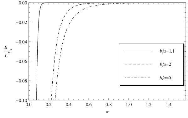
The results found by this strategy are shown in Figs. 4 and 5.


These graphs are very reminiscent of those found in Ref. [38] for the magnetodielectric wedge. In particular, we note that the energies are finite for all , but as , the limit corresponding to a Dirichlet boundary, the energy diverges as or ; the same phenomena was observed in Ref. [38] for the perfectly conducting wedge limit, treated previously in Ref. [37]. This energy should be observable as a torque on the two semitransparent plates, , which is, as expected, attractive. (The divergence associated with the apex of the wedge has been subtracted.)
IV Alternative calculation of Casimir energy for semitransparent wedge in an annulus
We start from the formula (2) for the Casimir energy in terms of the Green’s function,
| (30) |
where the trace denotes the integration over spatial coordinates, and we have again subtracted out the vacuum contribution. The Green’s function will satisfy the equation
| (31) |
while the free Green’s function satisfies the same equation with . Once again we specialize to the cylindrical geometry, but now defined in an annulus. Specifically, we require that the boundary conditions on the Green’s function are that it vanishes at and with , that is, it satisfies Dirichlet boundary conditions on two concentric circles. (We will see the necessity for both an inner and an outer boundary in the following.) If the potential has the form then we can use separation of variables to write the Green’s function as, in terms of the separation constant ,
| (32) |
The geometry we are considering is illustrated in Fig. 6.

Note that instead of expanding in eigenfunctions of as in Eq. (8), we have expanded in terms of radial eigenfunctions. (This cannot be done without the inner boundary—that is, this alternative separation works for an annulus but not for a disk.) The functions are normalized radial eigenfunctions of the eigenvalue problem,
| (33) |
with boundary values . The is the reduced Green’s function in the azimuthal coordinates that satisfies the equation
| (34) |
with periodic boundary conditions. Finally inserting Eq. (32) into Eq. (30) we get an expression for the vacuum energy
| (35) |
We can simplify the result considerably if we now make a Euclidean rotation from , make the substitution , and integrate out the angle in the - plane to get the expression for the energy per unit length
| (36) |
IV.1 The Radial Eigenvalue Problem
We see that we need an expression for the radial integral
| (37) |
where the s are the normalized eigenfunctions obeying the differential equation (33). The normalization is
| (38) |
To evaluate this integral we will use the identity (90). The boundary conditions are that ; this is only possible for discrete values of , namely, this is an eigenvalue condition for . Let be a solution to Eq. (33) which satisfies for all and . The normalized solution can then be written as
| (39) |
where
| (40) |
Now writing Eq. (33) as
| (41) |
we can see that is a total derivative given by Eq. (90). (We replace there.) The integral (40) is now trivial to carry out. We see that the value at the lower limit of integration is zero by our boundary condition that , and the second term on the right in Eq. (90) at the upper limit is zero by the eigenvalue condition . This gives the normalization constant as
| (42) |
IV.2 Argument Principle
Now we again use the argument principle (14), which we previously used for the angular eigenvalues; in this case the sum is over the radial eigenvalues, and the eigenvalue condition is given by . So we have occuring in the energy (36) the form
| (45) | |||||
The expression for the Casimir energy per length (36) is then given by
| (46) |
IV.3 The Radial Solutions
The differential equation (41) is the modified Bessel differential equation, of imaginary order. We need two independent solutions of this equation, which we could take to be and , given by Eq. (25). Now we want to find the solution that is zero for for all values of and . An obvious solution is
| (47) |
where
| (48) |
is the function initially called in Ref. [38]; here this is a more convenient choice, in that both and are even in .
IV.4 Reduced Green’s Function
We also need the reduced Green’s function in the angular coordinates. The free Green’s function is easily found to be
| (49) |
If we assume a single -function potential then the Green’s function is
| (50) |
which is defined for and in the interval .
IV.5 Casimir Energy
The final form for the Casimir energy for a single radial -function potential in the annular region is
| (53) | |||||
This result may also be obtained by the multiple scattering formalism [47], which says that
| (54) |
the latter form being a useful form for a single potential. We see that Eq. (53) exactly corresponds to this if we integrate by parts on and :
| (55) |
We can check this result by taking the limit as and get very large, but with fixed distance between the circles. In this limit this result should reproduce the case of a single semitransparent plane between two parallel Dirichlet planes, as illustrated in Fig. 7.

The energy in that case should be
| (56) |
where . If we use the argument principle we can write it as
| (57) |
The square root divided out in the logarithm is present to remove the spurious square-root singularity. It should be noted that both of these expressions (53) and (57) are divergent, but the divergence is simply the self-energy divergence always present with a single plane.
It is straightforward to prove that Eq. (53) reduces to Eq. (57) in the appropriate limit. The second logarithm in the former becomes, in the limit , simply so that suggests the correspondence
| (58) |
And the leading uniform asymptotic expansion of the modified Bessel functions [45, 46] gives
| (59) |
where , , , and
| (60) |
(The latter function is a continuation of a function usually called , but we have already used that symbol repeatedly.) This result holds true for , but an equivalent form, obtained by analytic continuation, holds for . (See Appendix B.) Then the derivative with respect to term in Eq. (53) becomes
| (61) |
so with the substitutions (58), and the observation that
| (62) |
we exactly recover the Casimir energy for a semitransparent plate between two Dirichlet plates (57).
It is also easy to check that the energy (53) agrees with the expression for the energy given by the more conventional approach described in Sec. II. The latter is
| (63) | |||||
This equivalence may be easily shown by seeing that the integrand is odd in , because
| (64) |
and then rotating the contour from that shown in Fig. 2 to that in Fig. 3, which may then be transformed to that shown in Fig. 8, by changing to on the negative imaginary axis. Thus the contour in the plane is transformed to in the plane appearing in Eq. (53) (except traversed in the opposite sense), and the equivalence is established.

IV.6 Interaction Between Two Semitransparent Planes
If we want to look at an explicitly finite quantity we will need to look at the interaction energy between two semitransparent planes. The geometry is illustrated in Fig. 9.

We will use a slightly different form of the energy for this, based on the multiple-scattering formalism [47]:
| (65) |
The subscripts on the s represent the potentials , and . The Green’s functions with superscript represent the interaction with only a single potential . By using Eq. (32), we can greatly simplify the interaction energy to
| (66) |
We already have an expression for , given in Eq. (50). Using the latter we can write
| (67) |
This exactly agrees with Eq. (23).
Using the argument principle to replace the sum we then get the Casimir energy of two semitransparent plates in a Dirichlet annulus, the immediate generalization of the Casimir energy (55) for a single plate,
| (68) |
A limiting case when , , fixed, should be two perpendicular semitransparent planes, a distance apart, sandwiched between Dirichlet planes, similar to the single plate situation treated in the subsection above. A similar formula should then be
| (69) |
As in the case of a single plate, this limiting form is immediately obtained from Eq. (68).
Finally, we verify that we obtain the expression (24) for the wedge geometry. To do this, we must include the modes exterior to the outer cylinder (with the wedge extended to infinity as in Fig. 1) and subtract the energy present if the outer cylinder were not present. This means that the radial dispersion function determining the azimuthal eigenvalues becomes
| (70) |
The extended annular energy is then given by Eq. (68) with . We now can distort the contour to one lying along the imaginary axis as shown in Fig. 3, , (because the second logarithm in Eq. (68) falls off exponentially fast for ), and then using the small argument expansion, for real ,
| (71) |
This means for small and real the first logarithm in Eq. (68) is , which is just what was encountered in Eq. (17). We then fold the integral to encircle the positive real axis as in Fig. 8 and integrate by parts in and . In this way the form (16) is reproduced (with ), which leads to the final expression (24).
IV.7 Numerical Evaluation of the Casimir Energy for Two Dirichlet Planes in an Annulus
The Casimir energy in Eq. (66) is a quickly converging function so it should be easy to evaluate. However, it can be difficult to evaluate the eigenvalues, which become functions of the wavenumber and a natural number . We can get around this problem, again, by exploiting the argument principle in order to get a contour integral in the complex plane, as in Eq. (68). We cannot integrate along the real line because of the poles introduced when we use the argument principle, and unlike with the wedge we cannot open along the imaginary axis, because the integral then becomes divergent. So a simple choice is then to let the integration run along the angles of and in the complex plane. Identifying from Eq. (47), and writing we have
| (72) |
Here we have used the property that , and . The value of is obtained as a numerical solution to the differential equation. Using this technique we can obtain a numerical energy in about 1 cpu-second. The results of this calculation are found in Fig. 10.
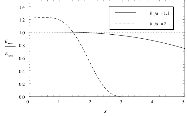
Again we would like to compare to known results, so Fig. 11 is a graph of the ratio of the energies of an annular piston to a rectangular piston of similar dimension. The rectangular piston is constructed so it has the same finite width as the annular piston, and the separation distance is the mean distance between the annular plates,
| (73) |
The results make a certain amount of physical sense. The energy of the annular piston is greater than that of the rectangular piston for small separation because the inner edge of the annular piston is closer, and will contribute more to the energy. However as the annular piston gets further away, the other side of the piston will start to contribute and lower the overall energy. In addition we see that the small ratio piston is much closer to the rectangular piston for small separations than a larger ratio, and in the plateau region for small separations, for vs. for . These numbers are quite closely reproduced by the ratio of the proximity force approximate value of the energy for tilted plates to the energy for parallel plates (ignoring the sidewalls) for small tilt angles,
| (74) |
V Theta dependent potentials
Instead of considering, as usually done, spherically or cylindrically symmetric potentials, in this paper we have been examining potentials depending on the angles. In particular, in two dimensions, in order for separation of variables to work, we have been considering the operator
| (75) |
with given in Eq. (1). The advantage of this potential is that a closed form for the secular equation can be given, see Eq. (11). But what can be said for other potentials ? The relevant equations for the two-dimensional Green’s function are still Eqs. (5)-(10b). In particular, for the angular eigenfunctions we still have
| (76) |
where is the separation constant. The separation constant is determined from the boundary condition in . For a smooth potential one imposes periodic boundary conditions, and this is what we concentrate on for concreteness.
Note, that the only information from Eq. (76) that enters Eq. (9) for the radial reduced Green’s function is the separation constant . From Eq. (76) its square can be considered the eigenvalue of
| (77) |
with periodic boundary conditions. For a nontrivial potential no explicit form of will be known. But also in general a transcendental equation determining the eigenvalues can be obtained; we follow Ref. [48]. In order to formulate this equation let be the fundamental matrix of Eq. (76). That is, let and be two linearly independent solutions of Eq. (76). With , the fundamental matrix is
where we choose the normalizations such that With these definitions and normalizations, the equation determining the eigenvalues reads
| (81) |
The solutions to this equation have to be used in Eq. (9). The Casimir energy expressions (16) and (17) then remain valid, once the appropriate radial reduced Green’s function is used and given in Eq. (81) is substituted. Once is specified this allows, in principle, for a numerical evaluation of the Casimir energy when suitable subtractions are performed.
Acknowledgements.
This material is based upon work supported by the National Science Foundation under Grants Nos. PHY-0554926 (OU) and PHY-0757791 (BU) and by the US Department of Energy under Grants Nos. DE-FG02-04ER41305 and DE-FG02-04ER-46140 (both OU). We thank Simen Ellingsen, Iver Brevik, Prachi Parashar, Nima Pourtolami, and Elom Abalo for collaboration. Part of the work was done while KK enjoyed the hospitality and partial support of the Department of Physics and Astronomy of the University of Oklahoma. Thanks go in particular to Kimball Milton and his group who made this very pleasant and exciting visit possible.Appendix A An Integral Theorem
It may be useful to see explicitly how the trace of the subtracted reduced Green’s function turns into a derivative of a logarithm, as in Eq. (17). Consider a Green’s function for a one-dimensional problem described by the differential equation
| (82) |
where is a -function potential,
| (83) |
The problem is defined on the interval , where at the boundaries satisfies Dirichlet boundary conditions,
| (84) |
If the potential , let the corresponding Green’s function be denoted by .
Let us solve this problem in terms of two independent solutions of the homogeneous equation
| (85) |
Let be such a solution that vanishes at the left boundary, , and be an independent solution that vanishes at the right boundary, , and let them be normalized so that the Wronskian is
| (86) |
Then the “free” Green’s function is
| (87) |
and the full Green’s function has the form
| (88) |
Now, it is easy to prove that
| (89) |
It is immediate that any two solutions of the differential equation (85) and satisfy
| (90) |
and therefore the following indefinite integral follows:
| (91) |
where .
Now we can evaluate the trace of the interaction part of the Green’s function,
| (92) | |||||
This is the expected expression. As shown in Sec. IV.5, this is just the expected multiple scattering result. In the Dirichlet limit , this agrees with the Bessel function result (17), where ; although in that case the boundary condition is not Dirichlet at the origin, .
Appendix B Modified Bessel Functions of Pure Imaginary Order
In this work we encountered the following differential equation
| (93) |
which is the modified Bessel equation, with the wrong sign for the order parameter . The solutions are then obviously modified Bessel functions of imaginary order. So we might choose as the independent pair of solutions the modified Bessel function of the first kind, of positive and negative pure imaginary order and . However the ’s are not numerically satisfactory functions; their values for real are complex, and the phase is dependent. A standard pair of functions can be defined as
| (94a) | |||||
| (94b) | |||||
The is the standard modified Bessel function of the second kind, also called the Macdonald function. Both and are real for real values of and . For a fixed , both and oscillate with relatively constant amplitude for and they die or grow exponentially for respectively. The limiting behaviors are given in this appendix; see Refs. [45, 46]. Although this definition of is convenient in Sec. II, for the considerations of Sec. IV, the in Eq. (94b) introduces spurious singularities, and it is more convenient there to simply use
| (95) |
also called in Ref. [38]. In the following we will give the behaviors of and .
B.1 Small Argument
For fixed , in the limit as ,
| (96a) | |||||
| (96b) | |||||
where is given by
| (97) |
B.2 Large Argument
For fixed and large argument we have
| (98a) | |||||
| (98b) | |||||
for arbitrary .
B.3 Uniform Asymptotic Expansion
The uniform asymptotic expansions are for both large order and argument. For fixed we have for the leading behavior
| (99a) | |||||
| (99b) | |||||
where the and are the Airy functions of the first and second kinds respectively, and is given by the relation
| (100) |
For we can use the behavior of the Airy functions for large negative argument to simplify the expressions,
| (101a) | |||||
| (101b) | |||||
If we choose the branch cut for equation (100) such that is a continuous real function of , then for we can simplify the expressions to read
| (102a) | |||||
| (102b) | |||||
where is the natural extension of
| (103) |
References
- [1] H. B. G. Casimir, Proc. Kon. Ned. Akad. Wetensch. 51, 793 (1948).
- [2] K. A. Milton, The Casimir Effect: Physical Manifestations of the Zero-Point Energy (World Scientific, Singapore, 2001).
- [3] K. A. Milton, J. Phys. A: Math. Gen. 37, R209 (2004).
- [4] S. K. Lamoreaux, Rep. Prog. Phys. 68, 201 (2005).
- [5] S. Y. Buhmann and D.-G. Welsch, Prog. Quantum Electron. 31, 51 (2007).
- [6] M. Bordag, G. L. Klimchitskaya, U. Mohideen, V. M. Mostepanenko, Advances in the Casimir Effect (Oxford, 2009).
- [7] L. L. DeRaad, Jr. and K. A. Milton, Ann. Phys. 186, 229 (1981).
- [8] I. Brevik and G. H. Nyland, Ann. Phys. 230, 321 (1994).
- [9] P. Gosdzinsky and A. Romeo, Phys. Lett. B 441, 265 (1998).
- [10] K. A. Milton, A. V. Nesterenko and V. V. Nesterenko, Phys. Rev. D 59, 105009 (1999).
- [11] G. Lambiase, V. V. Nesterenko and M. Bordag, J. Math. Phys. 40, 6254 (1999).
- [12] I. Cavero-Peláez and K. A. Milton, Ann. Phys. 320, 108 (2005); J. Phys. A. 39, 6225 (2006).
- [13] A. Romeo and K. A. Milton, Phys. Lett. B 621, 309 (2005); J. Phys. A 39, 6703 (2006).
- [14] I. Brevik and A. Romeo, Phys. Scripta 76, 48 (2007).
- [15] I. Cavero-Peláez, K. A. Milton and K. Kirsten, J. Phys. A 40, 3607 (2007).
- [16] J. S. Dowker and G. Kennedy, J. Phys. A 11, 895 (1978).
- [17] D. Deutsch and P. Candelas, Phys. Rev. D 20, 3063 (1979).
- [18] I. Brevik and M. Lygren, Ann. Phys. 251, 157 (1996).
- [19] I. Brevik, M. Lygren and V. Marachevsky, Ann. Phys. 267, 134 (1998).
- [20] I. Brevik, K. Pettersen, Ann. Phys. 291, 267 (2001).
- [21] V. V. Nesterenko, G. Lambiase and G. Scarpetta, Ann. Phys. 298, 403 (2002).
- [22] H. Razmi, S. M. Modarresi, Int. J. Theor. Phys. 44, 229 (2005).
- [23] V. M. Mostepanenko and N. N. Trunov, The Casimir Effect and Its Applications (Oxford University Press, Oxford, 1997).
- [24] V. V. Nesterenko, G. Lambiase and G. Scarpetta, J. Math. Phys. 42, 1974 (2001).
- [25] V. V. Nesterenko, I. G. Pirozhenko and J. Dittrich, Class. Quantum Grav. 20, 431 (2003).
- [26] A. H. Rezaeian and A. A. Saharian, Clas. Quant. Grav. 19, 3625 (2002).
- [27] A. A. Saharian, Eur. Phys. J. C 52, 721 (2007).
- [28] A. A. Saharian, in The Casimir Effect and Cosmology: A volume in honour of Professor Iver H. Brevik on the occasion of his 70th birthday, S. Odintsov et al. (eds.) (Tomsk State Pedagogical University Press, Tomsk, Russia, 2008), p.87, preprint hep-th/0810.5207.
- [29] A. A. Saharian and A. S. Tarloyan, J. Phys. A. 38, 8763 (2005).
- [30] A. A. Saharian and A. S. Tarloyan, Ann. Phys. (N.Y.) 323, 1588 (2008).
- [31] G. Barton, Proc. R. Soc. London 410, 175 (1987).
- [32] S. C. Skipsey, G. Juzeliūnas, M. Al-Amri, and M. Babiker, Optics Commun. 254, 262 (2005).
- [33] S. C. Skipsey, M. Al-Amri, M. Babiker, and G. Juzeliūnas, Phys. Rev. A, 73, 011803(R) (2006).
- [34] T. N. C. Mendes, F. S. S. Rosa, A. Tenório and C. Farina, J. Phys. A 41, 164029 (2008).
- [35] F. S. S. Rosa, T. N. C. Mendes, A. Tenório and C. Farina, Phys. Rev. A 78, 012105 (2008).
- [36] C. I. Sukenik, M. G. Boshier, D. Cho, V. Sandoghdar and E. A. Hinds, Phys. Rev. Lett. 70, 560 (1993).
- [37] I. Brevik, S. Å. Ellingsen and K. A. Milton, Phys. Rev. E 79, 041120 (2009).
- [38] S. Å. Ellingsen, I. Brevik, and K. A. Milton, Phys. Rev. E 80, 021125 (2009).
- [39] N. G. van Kampen, B. R. A. Nijboer and K. Schram, Phys. Lett. 26A, 307 (1968).
- [40] M. Bordag, E. Elizalde, and K. Kirsten, J. Math. Phys. 37, 895 (1996).
- [41] V. A. Parsegian, Van Der Waals Forces (Cambridge: Cambridge Univ. Press, 2006) §L3.3.
- [42] I. Brevik, B. Jensen, and K. A. Milton, Phys. Rev. D 64, 088701 (2001).
- [43] V. V. Nesterenko, J. Phys. A, 39, 6609 (2006).
- [44] V. V. Nesterenko, J. Phys. A, 41, 164005 (2008).
- [45] T. M. Dunster, SIAM J. Math. Anal. 21, 995 (1990).
- [46] F. W. J. Olver, Asymptotics and Special Functions, (Academic Press, New York, 1974), Chaps. 10–12.
- [47] K. A. Milton and J. Wagner, J. Phys. A 41, 155402 (2008).
- [48] K. Kirsten and A.J. McKane, J. Phys. A: Math. Gen., 37, 4649 (2004).