Coherent sets for nonautonomous dynamical systems
Abstract
We describe a mathematical formalism and numerical algorithms for identifying and tracking slowly mixing objects in nonautonomous dynamical systems. In the autonomous setting, such objects are variously known as almost-invariant sets, metastable sets, persistent patterns, or strange eigenmodes, and have proved to be important in a variety of applications. In this current work, we explain how to extend existing autonomous approaches to the nonautonomous setting. We call the new time-dependent slowly mixing objects coherent sets as they represent regions of phase space that disperse very slowly and remain coherent. The new methods are illustrated via detailed examples in both discrete and continuous time.
1 Introduction
The study of transport and mixing in dynamical systems has received considerable attention in the last two decades; see e.g. [31, 46, 1, 47] for discussions of transport phenomena. In particular, the detection of very slowly mixing objects, known variously as almost-invariant sets, metastable sets, persistent patterns, or strange eigenmodes, has found wide application in fields such as fluid dynamics [34, 30, 35], ocean dynamics [21, npg], astrodynamics [4], and molecular dynamics [9, 41]. A shortcoming of this prior work, based around eigenfunctions of Perron–Frobenius operators (or transfer operators, or evolution operators) is the restriction to autonomous systems or periodically forced systems. In this work, we extend the notions of almost-invariant sets, metastable sets, persistent patterns, and strange eigenmodes to time-dependent Lagrangian coherent sets. These coherent sets form a time parameterised family of sets that approximately follow the flow and disperse very slowly; in other words they stay coherent. Coherent sets are the natural nonautonomous analogue to almost-invariant sets.
The standard dynamical systems model of transport assumes that the motion of passive particles are completely determined by either an autonomous or a time-dependent vector field. Traditional approaches to understanding transport are based upon the determination of the location of geometric objects such as invariant manifolds. In the autonomous setting, an invariant manifold of one dimension less than the ambient space will form an impenetrable transport barrier that locally partitions the ambient space. In the periodically-forced setting, primarily in two-dimensional flows, it has been shown that slow mixing in the neighbourhood of invariant manifolds is sometimes controlled by “lobe dynamics” [36, 37, 46]. In the truly non-autonomous, or aperiodically forced setting, finite-time hyperbolic material lines [24] and surfaces [25] have been proposed as generalisations of invariant manifolds that form barriers to mixing. These material lines and surfaces are known as Lagrangian coherent structures; see also [42] for an alternative definition. The geometric approach can often be used to find co-dimension 1 sets (coherent structures) that form boundaries of coherent sets.
An alternative to the geometric approach is the ergodic theoretic approach, which attempts to locate almost-invariant sets (or metastable sets) directly, rather than inferring their location indirectly from their boundaries. The basic tool is the Perron–Frobenius operator (or transfer operator). Real eigenvalues of this operator close to 1 correspond to eigenmodes that decay at slow (exponential) rates. Almost-invariant sets are heuristically determined from the corresponding eigenfunctions as sets of the form or for thresholds . Such an approach arose in the context of smooth autonomous maps and flows on subsets of [7, 6] about a decade ago. Further theoretical and computational extensions have since been constructed [17, 15, 16]. A parallel series of work specific to time-symmetric Markov processes and applied to identifying molecular conformations was developed in [40, 8, 9] and surveyed in [41].
There have been some recent studies of the connections between slow mixing in periodically driven fluid flow and eigenfunctions of Perron–Frobenius operators. Liu and Haller [30] observe via simulation a transient “strange eigenmode” as predicted by classical Floquet theory. Pikovsky and Popovych [34, 35] numerically integrated an advection-diffusion equation to simulate the evolution of a passive scalar, observing that it is the sub-dominant eigenfunction of the Perron–Frobenius operator that describes the most persistent deviation from the unique steady state.
The Perron–Frobenius operator based approach has been successful in a variety of application areas, however, as the key mathematical object is an eigenfunction, there is no simple extension of the method to systems that have nonperiodic time dependence11 1 A relevant analogy to see this is the following. Consider repeated application of a single matrix . The eigenvectors of provide information on directions of exponential growth/decay specified by the corresponding eigenvalues. Similarly, the eigenvectors of a product of matrices describe directions of exponential growth/decay, specified by the eigenvalues of the product, under repeated application of this matrix product. However, the directions of exponential growth/decay under a non-repeating product cannot be in general be found as eigenvectors of some matrix.
Indeed, Liu and Haller [30] state that:
“…strange eigenmodes may also be viewed as eigenfunctions of an appropriate Frobenius-Perron operator…This fresh approach offers an alternative view on scalar mixing, but leaves the questions of completeness and general time-dependence open.”
It is this question of general time-dependence that we address in the current work. We extend a standard formalism for random dynamical systems to the level of Perron–Frobenius operators to create a Perron–Frobenius operator framework for general time-dependence. We also state an accompanying numerical algorithm, and demonstrate its effectiveness in identifying strange eigenmodes and coherent sets.
An outline of the paper is as follows. In Section 2 we formalise the notions of nonautonomous systems in both discrete and continuous time. In Section 3 we describe a Galerkin projection method that we will use to produce finite matrix representations of Perron–Frobenius operators. In Section 4 we define the critical constructions for the nonautonomous setting. We show that the nonautonomous analogues of strange eigenmodes are described by the “Oseledets subspaces” or “Lyapunov vectors” corresponding to compositions of the projected Perron–Frobenius operators. In Section 5 we describe in detail a numerical algorithm to practically compute these slowly decaying modes, and demonstrate that in the continuous time setting, these modes vary continuously in time. Our numerical approach is illustrated firstly in the discrete time setting with an aperiodic composition of interval maps, and secondly in the continuous time setting with an aperiodically forced flow on a cylinder. Section 6 provides some further background on almost-invariant sets and coherent sets and Section 7 describes a new heuristic to extract coherent sets from slowly decaying modes in the nonautonomous setting. This heuristic is then illustrated using the examples from Section 5.
2 Nonautonomous Dynamical Systems
We will treat time dependent dynamical systems on a smooth compact -dimensional manifold , in both discrete and continuous time. In order to keep track of “time” we use a probability space , with the passing of time controlled by an ergodic automorphism preserving (ie. for all ). We require this somewhat more complicated description of time for technical reasons: to run the ergodic-theoretic arguments in Theorem 1 that guarantee the existence of the nonautonomous analogues of strange eigenmodes. The requirement that be an ergodic probability measure rules out obvious choices for and : (i) in discrete time, and , and (ii) in continuous time, and . In both (i) and (ii), there is no ergodic probability measure on preserved by . In the next two sections, we will introduce suitable examples of and and describe the nonautonomous systems they generate.
2.1 Discrete time – Maps
In the discrete time setting, we will think of , and as a left shift on defined by , where . We assume that is ergodic with respect to . Let be a collection of (possibly non-invertible) piecewise differentiable maps on a compact manifold . For brevity, we will sometimes write in place of . We will define a nonautonomous dynamical system by map compositions of the form . Define
For (resp. ), represents the forward time (resp. backward time) -fold application of the nonautonomous dynamics to the point initialised at “time” . Whenever is non-invertible, will represent the finite set of all preimages of . We call a map cocycle.
Definition 1.
Endow with the Borel -algebra and let be a probability measure on . We call an invariant measure if for all .
This definition of an invariant measure is stricter than is usual for random or nonautonomous dynamical systems (e.g. [2, Definition 1.4.1]). More generally, one may allow sample measures and insist that for all .
Example 1 (Aperiodic map cocycle).
We construct a map cocycle by the composition of maps from a collection according to sequences of indices . The collection consists of expanding maps of the circle , which we think of as with endpoints identified. The sequence space is given by
with adjacency matrix
Elements of correspond to bi-infinite paths in the graph Figure 1.

The shift is a subshift of finite type. A Borel -algebra is generated by the length-one cylinder sets , , and by giving equal measure to these four cylinder sets, we generate a shift-invariant probability measure .
The maps of are defined in terms of a continuous piecewise-linear map , which has almost-invariant sets (see Definition 5, Section 6) and for close to zero. Define
where values are taken modulo . Figure 2 shows a graph of .

Let , , be close to zero, for example . We now construct the map from , for as follows:
where is the rotation ; see Figure 3.

Let denote normalised Lebesgue measure on . To each map we associate a Perron–Frobenius operator defined by . The operator is a linear operator that acts on integrable functions in analogy to the action of on points. If represents a density function for an ensemble of initial conditions, then represents the density function of the ensemble after the action of has been applied to the ensemble. The map cocycle naturally generates a Perron–Frobenius cocycle . This composition of Perron–Frobenius operators capture the action on a function after iterations of the non-autonomous system.
2.2 Continuous time – Flows
Let be a sufficiently regular vector field. More precisely, we suppose that satisfies the conditions of [2, Theorem 2.2.2], which will guarantee the existence of a classical solution of the nonautonomous ODE , .
To be concrete about the probability space in the continuous time setting, we may set , , and consider an autonomous ODE on . Denote the flow for this ODE by and suppose that preserves the probability measure ; that is, for all . Thus, the autonomous, aperiodic flow drives the nonautonomous ODE
| (1) |
We think of points as representing generalised time. We assume that is ergodic in the sense that if for some and for all then or 1.
Denote by the flow for (1). The flow satisfies .
Definition 2.
Endow with the Borel -algebra and let be a probability measure on . We call an invariant measure if for all and .
Remark 1.
In Definition 2 we are insisting that is preserved at all “time instants”. As in the discrete time setting, more generally one may allow and insist that . However, as we will soon begin to focus on coherent sets rather than invariant measures, we will restrict the invariant measure to a “time independent” measure for clarity of presentation. This is perfectly reasonable for one of the main applications we have in mind, namely, aperiodically driven fluid flow where Lebesgue, and volume is preserved by the flow at all times.
Example 2.
Consider the following nonautonomous system on a cylinder . Let denote the flow for the driving system generated by the Lorenz system of ODEs (2)–(4) with standard parameters , , .
| (2) | |||||
| (3) | |||||
| (4) |
It is well known that this Lorenz flow possesses an SBR measure [44]. Let the time-dependent vector field generate our non-autonomous ODE . Explicitly,
| (5) | |||||
| (6) |
with , , . We set initial condition and take the -coordinate of the Lorenz driving system to represent the generalized time for the vector field . We use a scaling factor of so that the temporal and spatial variation of is similar to that of the “actual” time . Since is differentiable and bounded on for all , classical solutions of the nonautonomous ODE (5)–(6) exist. The system (2)–(6) uniquely generates an RDS, see [2, Theorem 2.2.2]. In Figure 4 we demonstrate a trajectory of three different initial points.

We may define a family of Perron–Frobenius operators as for . This family is a semigroup in as .
3 Galerkin projection and matrix cocycles
Let where is a partition of into connected sets of positive Lebesgue measure. Define a projection as
| (7) |
Following Ulam [45], in the sequel we will consider the finite rank operators and , and the matrix representations of the restrictions of and to . We denote these matrix representations (under multiplication on the right) by and . Extending Lemma 2.3 [29] in a straightforward way to the nonautonomous setting, one has
| (8) |
and
| (9) |
In particular, these matrices are numerically accessible.
Remark 2.
The matrices and generate matrix cocycles
| (10) |
and
| (11) |
4 Discretised Oseledets functions and the Multiplicative Ergodic Theorem
In periodically driven flows, Liu and Haller [30] and Pikovsky and Popovych [34], observed that certain tracer patterns persisted for long times before eventually relaxing to the equilibrium tracer distribution. Pikovsky and Popovych [34] recognised these patterns as graphs of eigenfunctions of a Perron–Frobenius operator corresponding to an eigenvalue . These eigenfunctions decay over time and the closer is to 1, the slower the decay and the more slowly an initial tracer distribution will relax to equilibrium. We now develop a framework for the considerably more difficult aperiodic setting.
Consider some suitable Banach space of real valued functions; is the function class in which we search for slowly decaying functions. Suppose that the norm is chosen so that for each and , the operator is Markov; that is, for all and . For , we calculate the following limit:
| (12) |
We refer to as the Lyapunov exponent of . If decays under the action of the Perron–Frobenius operators at a geometric rate of , , then . The closer is to 1, the slower the decay. The extreme case of (no decay) is exhibited when is the density of the invariant measure that is common to all maps in our nonautonomous dynamical system. We define the Lyapunov spectrum . In the aperiodic setting the new mathematical objects that are analogous to strange eigenmodes and persistent patterns will be called Oseledets functions.
Definition 3.
Oseledets functions correspond to for which (i) is near zero and (ii) the value is an isolated point in the Lyapunov spectrum.
By considering , the actions of and are described by and , respectively. We may replace and in (12) by and , respectively, to obtain a standard setting where the possible values of are the Lyapunov exponents of cocycles of matrices, and
| (13) |
and
| (14) |
exist for almost-all , and consist of at most isolated points, . Of particular interest to us is the function (or ) in , which represents the function that decays at the slowest possible geometric rate .
Remark 3.
In certain settings, this matrix cocycle exactly captures all large isolated Lyapunov exponents of the operator cocycle . One such setting is a map cocycle formed by composition of piecewise linear expanding maps with a common Markov partition ; see [19].
The following example illustrates the concept of Lyapunov spectrum and Oseledets functions in the familiar autonomous setting. For the remainder of this section, we adopt the discrete time notation of and .
Example 3 (“Autonomous” single map).
In [5] individual maps are constructed for which the Perron–Frobenius operator has at least one non-unit isolated eigenvalue when acting on the Banach space . A single autonomous map may be regarded as a cocycle over a one-point space , and so we may drop the dependence on in notation. Keller [27] shows that for a piecewise expanding map of the interval , the spectrum of the associated Perron–Frobenius operator has an essential spectral radius equal to the asymptotic local expansion rate , and that there are at most countably many spectral points, each isolated, of modulus greater than . In order to have an isolated spectral point, we construct a map of which has an almost-invariant set (see Definition 5). The relation between almost-invariant sets and isolated eigenvalues was noted in [7]. Consider the partition , where . Given , any map defined by
| (15) |
is Markov with respect to . Here we take ; see Figure 5. Notice that there is a low transfer of mass between the two intervals and . Since is a Markov partition for , the space of characteristic functions is an invariant subspace of for the Perron–Frobenius operator of . Thus the action of on is represented by the matrix
which has non-zero eigenvalues . The map is piecewise affine with constant slope and so the logarithm of the local expansion rate is .
The eigenvalue of thus gives rise to an isolated point in the Lyapunov spectrum . The corresponding Oseledets function is given by , where is the eigenvector of corresponding to the eigenvalue , see Figure 5.
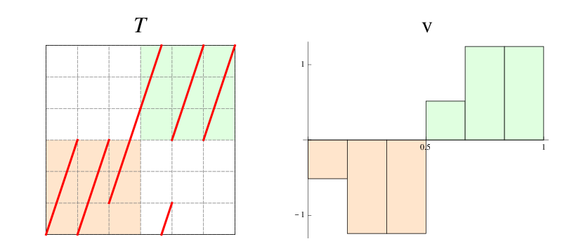
Since , this means that is the unique isolated Lyapunov exponent in . Note that the set corresponds to the set . We will discuss this property further in Section 7.
Example 4 (Periodic map cocycle).
We construct a periodic map cocycle from a collection of maps with a common Markov partition. The map cocycle is formed by cyclically composing three maps of . Consider the sequence space where . We consider , where is given by (15) with parameter , where
see Figure 6.

As in Example 3 we look for Lyapunov exponents that are strictly greater than the logarithm of the asymptotic local expansion rate
| (23) |
As each map is piecewise affine with constant slope , the logarithm of the local expansion rate is . Note also that approximately maps to , then maps approximately to , and finally maps approximately back to . Each map leaves the space from Example 3 invariant, and thus the Perron–Frobenius operator of restricted to has matrix representation , where , , are respectively
The triple product has non-zero eigenvalues and . Since , its associated eigenvector satisfies . Since , , are cyclic permutations of the factors of , they share the same eigenvalues, and in particular . Thus is an isolated Lyapunov exponent of for each . Associated to the eigenvalue , the matrices , , have corresponding eigenvectors . The three vectors , , generate the periodic Oseledets functions , see Figure 7.

In the nonautonomous setting, we can no longer easily construct Oseledets functions as eigenfunctions of a single operator, or eigenvectors of a single matrix. In fact, the Oseledets functions are themselves (aperiodically) time dependent in the nonautonomous setting. Our model of Oseledets functions for nonautonomous systems is, as the name suggests, built around the Multiplicative Ergodic Theorem, see e.g. [2, Chapter 3, §4]. We now state a strengthened version [19] of the Multiplicative Ergodic Theorem that we require for our current purposes.
Theorem 1 ([19]).
Let be an invertible ergodic measure-preserving transformation of the space . Let be a measurable family of matrices satisfying
Then there exist and dimensions , with , and a measurable family of subspaces such that for almost every the following hold:
- 1.
;
- 2.
;
- 3.
(with equality if );
- 4.
for all , one has
The subspaces are the general time-dependent analogues of the vectors and of Examples 3 and 4, respectively. We may explicitly construct a slowest decaying discrete Oseledets function as , where . In the sequel, for brevity we will often call a subspace or a function, recognising its dual roles.
Remark 4.
We remark that if , , and , the family of vectors is the unique22 2 Assume there is another family (up to scalar multiples) with these properties. Then for some , , with . WLOG assume for some and all , but that for all and all . Then in Theorem 1, a contradiction. (up to scalar multiples) family of vectors in with the properties that
- 1.
, ,
- 2.
for some , .
Remark 5.
Theorem 1 strengthens the standard version of the MET for one-sided time with noninvertible matrices (see e.g. [2, Theorem 3.4.1]) to obtain the conclusions of the two-sided time MET with invertible matrices (see e.g. [2, Theorem 3.4.11]). In [2, Theorem 3.4.1], the existence of only a flag of Oseledets subspaces is guaranteed, while in [2, Theorem 3.4.11], the existence of a splitting is guaranteed. Theorem 1 above demonstrates existence of an Oseledets splitting for two-sided time with noninvertible matrices. This is particularly important for our intended application as the projected Perron–Frobenius operator matrices are non-invertible. Recent further extensions [froyland_lloyd_quas2] prove existence and uniqueness of Oseledets subpsaces for cocycles of Lasota-Yorke maps.
5 Numerical approximation of Oseledets functions
In the autonomous and periodic settings we have seen in Examples 3 and 4 that the subspaces were one-dimensional, and that the vectors could be simply determined as eigenvectors of matrices. For truly nonautonomous systems (those that are aperiodically driven), the Oseledets splittings are difficult to compute. In this section we outline a numerical algorithm to approximate the subspaces from Theorem 1. The algorithm is based on the push-forward limit argument developed in the proof of Theorem 1. To streamline notation, we describe the discrete time and continuous time setting separately.
5.1 Discrete time
We first describe a simple and efficient method to construct the matrix defined in (8).
Algorithm 1 (Approximation of , ).
- 1.
Partition the state space into a collection of connected sets of small diameter.
- 2.
Fix , , and and create a set of test points that are uniformly distributed over .
- 3.
For each calculate .
- 4.
Set
(43)
We now describe how to use the matrices to approximate the subspaces . An intuitive description of the ideas behind Algorithm 2 immediately follows the algorithm statement.
Algorithm 2 (Approximation of Oseledets subspaces at .).
- 1.
- 2.
Form
as an approximation to the standard limiting matrix
appearing in the Multiplicative Ergodic Theorem (see e.g. [2, Theorem 3.4.1(i)]).
- 3.
Calculate the orthonormal eigenspace decomposition of , denoted by , . We are particularly interested in low values of , corresponding to large eigenvalues .
- 4.
Define via the push forward under the matrix cocycle.
- 5.
is our numerical approximation to .
Here is the idea behind the above algorithm. If we choose large enough, the eigenspace should be close to the limiting () eigenspace . Vectors in the eigenspace experience stretching at a rate close to . Note that the eigenspace is the singular vector of the matrix , which experiences a “per unit time” average stretching from time to of . Choose some arbitrary and write with . Pushing forward by for large enough will result in dominating for . Thus, for large and we expect to be close to .
Remarks 1.
- 1.
Theorem 1 states that as .
- 2.
This method may also be used to calculate the Oseledets subspaces for two-sided linear cocycles, and may be more convenient, especially for large , than the standard method of intersecting the relevant subspaces of flags of the forward and backward cocycles.
The numerical approximation of the Oseledets subspaces has been considered by a variety of authors in the context of (usually invertible) nonlinear differentiable dynamical systems, where the linear cocycle is generated by Jacobian matrices concatenated along trajectories of the nonlinear system. Froyland et al. [18] approximate the Oseledets subspaces in invertible two-dimensional systems by multiplying a randomly chosen vector by (pushing forward) or (pulling back, where . Trevisan and Pancotti [trevisan_pancotti_98] calculate eigenvectors of for the three-dimensional Lorenz flow, increasing until numerical convergence of the eigenvectors is observed. Ershov and Potapov [12] use an approach similar to ours, combining eigenvectors of a with pushing forward under . Ginelli et al. [23] embed the approach of [18] in a QR-decomposition methodology to estimate the Oseledets vectors in higher dimensions. In the numerical experiments that follow, we have found our approach to work very well, with fast convergence in terms of both and .
5.2 Continuous time
As our practical computations are necessarily over finite time intervals, from now on, when dealing with continuous time systems, we will compute as rather than as . If the computation of can be done accurately (this will be discussed further in Section 5.5), then this representation should be closer to as there are fewer applications of .
We first describe a simple and efficient method to construct the matrix defined in (8).
Algorithm 3 (Approximation of , ).
- 1.
Partition the state space into a collection of connected sets of small diameter.
- 2.
Fix ,, and and create a set of test points that are uniformly distributed over .
- 3.
For each calculate .
- 4.
Set
(44)
The flow time should be chosen long enough so that most test points leave their partition set of origin, otherwise at the resolution given by the partition , the matrix matrix will be too close to the identity matrix. If the action of separates nearby points, as is the case for chaotic systems, clearly the longer the flow duration , the greater should be in order to maintain a good representation of the images by the test points.
Algorithm 4 (Approximation of Oseledets subspaces at .).
- 1.
Construct the Ulam matrices and from (44) for suitable and . The number represents the flow duration over which rate of decay is measured, while the number represents the duration over which the resulting “initial vectors” are pushed forward to better approximate elements of the .
- 2.
Form
as an approximation to the standard limiting matrix
appearing in the Multiplicative Ergodic Theorem (see e.g. [2, Theorem 3.4.1(i)]).
- 3.
Calculate the orthonormal eigenspace decomposition of , denoted by , . We are particularly interested in low values of , corresponding to large eigenvalues .
- 4.
Define via the push forward under the matrix cocycle.
- 5.
is our numerical approximation to .
5.3 Continuity of the Oseledets subspaces in continuous time
When treating continuous time systems, one may ask about the continuity properties of in . In the following we suppose that is one-dimensional. For large and , will approximate the most dominant Oseledets subspace at time . Suppose that we are interested in how this subspace changes from time to time for small . There are two ways to obtain information at time . Firstly, we can simply push forward slightly longer to produce . Secondly, we can compute slightly later at time to produce .
To compare the closeness of to and , we represent each as a function and make a comparison in the norm. We assume that is one-dimensional and define where is scaled so that . Let . Note that for some .
We firstly compare and .
Proposition 1.
as .
Proof.
Note that while . The proof will follow from the result that is a continuous semigroup; that is, for all , .
Lemma 1.
as for all and .
Proof.
The proof runs as a non-autonomous version of the discussion in Remark 7.6.2 [28]. Note that , where denotes the flow from in reverse time for duration . For the moment consider continuous . Since is at least for each (the derivative of wrt to is continuous with respect to and for each fixed ) by [2, Theorem 2.2.2 (iv)] and is compact, uniformly in as . Thus as . Since the continuous functions are dense in , as is compact (see e.g. [11] Lemma IV.8.19), one can approximate any by a continuous function and thus the result holds for all functions . ∎
Thus the result follows using Lemma 1 and the fact that . ∎
Now, let’s compare and .
Proposition 2.
as .
Proof.
This result is more difficult to demonstrate as we need to firstly compare with . To this end, consider
The right hand side converges to zero as by Lemma 1. This result implies that as in whatever matrix norm we choose. Thus as . By standard perturbation results, see e.g. [26, Theorem II.5.1], this implies that eigenvectors and are close for sufficiently small . Thus and are close in norm. Now we need to push both of these forward by . This will not increase the norm of the difference at all, so will also be small. ∎
5.4 Oseledets functions for a 1D discrete time nonautonomous system
We now examine the Oseledets functions for the system defined in Example 1. We consider the approximation of rank , which we obtain by Galerkin projection. We denote by the Ulam matrix representing the action of on functions . The matrices are constructed by following Algorithm 1 using .
We look for Oseledets functions for a particular aperiodic sequence . To generate an aperiodic sequence, let be the binary expansion of . Extend to an element of by setting for all . Define for each . Then and the central terms of are
| (45) |
where the dot denotes the zeroth term .
We calculate the eigenvalues of , where is defined as in (10), and find the top three to be
As in Examples 3 and 4, the maps are piecewise affine with constant slope three, and so . Thus and may approximate isolated Lyapunov exponents in .
We follow Algorithm 2 to approximate the second Oseledets subspace for , using , see Figure 8.

In order to confirm the effectiveness of Algorithm 2 we calculate the distance between the normalisations of the vectors and , for with . By property 3 of Theorem 1 this distance should be small if the family is well approximated. A logarithmic plot of against , see Figure 9, shows the fast convergence of to an Oseledets subspace.

In Section 7.2 we will see how to extract coherent sets from these functions.
5.5 Oseledets functions in a 2D continuous time nonautonomous system
We consider the following nonautonomous system on , :
| (46) |
This equation describes a travelling wave in a stationary frame of reference with rigid boundaries at and , where the normal flow vanishes [33, 39]. The streamfunction (Hamiltonian) of this system is given by
| (47) |
We set , , and the phase speed to . The velocity field is -periodic in the -direction, which allow us to study the flow on a cylinder. The velocity fields in a comoving frame for these parameters are shown in Figure 10. The closed recirculation regions adjacent to the walls ( and ) move in the positive -direction and are separated from the jet flowing regime by the heteroclinic loops of fixed points, which are given below.
This model can be simplified to an autonomous system with a steady streamfunction in the comoving frame by setting and . The steady streamfunction is then given by . Let and . In the comoving frame, the recirculation region at the wall contains an elliptic point and is bounded by the heteroclinic loop of the hyperbolic fixed points and . Similarly, those elliptic and hyperbolic points at the wall are , , and , respectively, see Figure 10. One may observe that there is a continuous family of invariant sets in the comoving frame as any fixed level set of the streamfunction bounds an invariant set. In a stationary frame these elliptic and hyperbolic points (and their heteroclinic loops) are just translated in the direction. That is, any fixed level set of the time-dependent streamfunction (47) is a (time-dependent) invariant manifold. We note, however, that the recirculation regions are distinguished from the remainder of the cylinder as they are separated from the jet flowing region, which has a different dynamical fate. In the subsequent sections we will perturb this somewhat “degenerate” system to destroy the continuum of invariant sets in the comoving frame and produce a small number of almost-invariant sets (see Definition 5) in the comoving frame, or coherent sets in the stationary frame).

5.5.1 A coherent family: Mixing case
We modify the traveling wave model in the previous section to allow mixing in the jet flowing region. We add a perturbation to the system in the following way:
| (48) |
Here, , where is generated by the Lorenz flow in Example 2 with initial point , , and the parameter function vanishes at the level set of the streamfunction of the unperturbed flow at instantaneous time t=0, i.e., , which divides the phase space in half. We set as this value is sufficiently large to ensure no KAM tori remain in the jet regime, but sufficiently small to maintain islands originating from the nested periodic orbits around the elliptic points of the unperturbed system.
We applied Algorithm 3 with , , , , and Algorithm 4 for and . By using a relatively large number of test points per grid box ( points per box ) we are able to flow for units of time and still well represent . Figure 11 shows that the resulting Oseledets functions highlight the remaining islands in the perturbed time-dependent flow. We calculate the eigenvalues of , where is defined as in (44), and find the top three to be

6 Invariant Sets, Almost-Invariant Sets, and Coherent Sets
We begin by briefly recounting some of the background relevant to almost-invariant sets. If (resp. ) is autonomous, then (resp. ) consists of a single point, and we may write (resp. ).
Definition 4.
In the autonomous setting, we call an invariant set if (resp. for all ).
The following definition generalises invariant sets to almost-invariant sets. In the continuous time case we define:
Definition 5.
Let be preserved by the autonomous flow . We will say that a set is -almost-invariant over the interval if
- 1.
(49) for all ,
- 2.
is connected.
If is almost-invariant over the interval , then for each , the probability (according to ) of a trajectory leaving at some time in , and not returning to at time is relatively small. In the discrete time setting, , and the obvious changes are made in Definition 5. By convention we ask that is connected; if is not connected, we consider each connected component to be an almost-invariant set for suitable .
We now begin to discuss the nonautonomous setting. The notion of an invariant set is extended to an invariant family.
Definition 6.
- 1.
Discrete time: We will call a family of sets , , , an invariant family if for all and .
- 2.
Continuous time: We will call a family of sets , , , an invariant family if for all and .
Motivated by a model of fluid flow, we imagine coherent sets as a family of connected sets with the property that the set is approximately mapped onto by iterations of the cocycle from “time” ; that is, . The definition of coherent sets combines the properties of almost-invariant sets and an invariant family. As we now have a family of sets we require one more property beyond those of Definition 5, in addition to modifying the almost-invariance property. In the continuous time case we define:
Definition 7.
Let be preserved by a flow and . Fix a . We will say that a family , , is a family of -coherent sets over the interval if:
- 1.
(50) for all and ,
- 2.
Each , is connected,
- 3.
for all ,
In discrete time, we replace (50) with
| (51) |
necessarily becomes 1, and we make the obvious changes to the other items in Definition 7.
We remark that by selecting some of positive measure and defining , , the family , is a family of 1-coherent sets. Such a family is not of much dynamical interest, as there is nothing distinguishing this family from one constructed with another connected subset . We are not interested in these constructions of coherent sets, and in practice the numerical algorithm we present in the next section is unlikely to find such sets for chaotic systems.
7 Coherent sets from Oseledets functions
We wish to find a family of sets so that
| (52) |
is large for . We may rewrite the RHS of (52) as
| (53) |
For (53) to be large we require .
Let us now make a connection with the Oseledets functions where obtained in Algorithm 4. In the following discussion, we scale so that for all . To convert the family of Oseledets functions into a family of coherent sets, we modify a heuristic due to [7] that has been successfully used in the autonomous setting. The heuristic is to set , . We show that is small for moderate and large ; we then heuristically infer that .
Proposition 3.
Let be the second largest Lyapunov exponent from Theorem 1 and a corresponding Oseledets function, normalised so that . Given an there is an so that implies .
Proof.
Given we know that there exists such that for all one has . Since and , one has . Thus . Since , one has . As and , we have and since preserves integrals, . Thus, . ∎
The preceding discussion heuristically addresses item 1. of Definition 7. Regarding item 2 of Definition 7, as we are extracting the sets from the Oseledets functions , the connectivity of the sets will depend on the regularity of the Oseledets functions. This is a delicate question and relatively little can be said formally at present. In the autonomous case, roughly speaking, one expects smooth eigenfunctions for Perron–Frobenius operators of smooth expanding systems [27, 38], and eigendistributions (smooth in expanding directions, distributions in contracting directions) in uniformly hyperbolic settings [3]. These properties may carry over to the non-autonomous setting; recent results in the bounded variation setting show they do [froyland_lloyd_quas2]. If a small amount of noise is added by postmultiplying the Perron–Frobenius operator by a smoothing (e.g. diffusion) operator, then the Oseledets functions must be smooth. This physical addition of a small amount of noise is one way to guarantee regularity of the Oseledets functions and connectivity of the associated coherent sets.
Finally we note that if one has and so we must have for all . Thus, item 3. of Definition 7 is satisfied by the choice . If , then it may be necessary to further tweak the choice of the to ensure that item 3. of Definition 7 is satisfied. This additional tweak is described in Algorithm 5.
7.1 A numerical algorithm
For a fixed time , we seek to approximate a pair of sets and for which
| (54) |
is maximal. The quantity is simply the fraction of -measure of that is covered by a pullback of the set over a duration of . For maximal coherence, we wish to find pairs , that maximise . We present a heuristic to find such a pair of sets based upon the vectors and corresponding to some Lyapunov spectral value close to 0. This heuristic is a modification of heuristics to determine maximal almost-invariant sets, see [17, 15, 20]. In the terminology of the prior discussion in §7, rather than setting , we allow or for some in the hope of finding with an even greater value of . This additional flexibility also permits a matching of and .
Algorithm 5 (To determine a pair of maximally coherent sets at times ).
- 1.
Determine and for some according to Algorithm 4.
- 2.
Set and , restricting the values of so that . These are sets constructed from grid boxes whose corresponding entry in the vectors is above a certain value.
- 3.
Define . Given a value of , determines the set that best matches the -measure of , as required by item 3 of Definition 7.
- 4.
Set . The value of is selected to maximise the coherence.
- 5.
Define and .
7.2 Coherent Sets for a 1D discrete time nonautonomous system
We return to the map cocycle and Perron–Frobenius cocycle described in Example 1 and identify coherent sets. We use two methods: firstly, inspection of the composition of maps as perturbations of maps with invariant sets, and secondly using the general method of Algorithm 5.
The map cocycle is defined in terms of a map which has an almost-invariant set, and this gives rise to a family of coherent sets in the following way. Recall the definitions of the maps , and shift space determined by the adjacency matrix . The maps have the property that if , then any inner factors cancel in . More generally, for any , we have cancellation of all intermediate factors:
| (55) |
where are given by
For the map , the interval is invariant. Moreover, is almost-invariant for with . By (55), we if we set
| (56) |
then
Thus is a family of -coherent sets with . In the same way, the invariant set of leads to a family of -coherent sets with the same .
In order to demonstrate the methods of this article, we now show how Algorithm 5 can be used. We may use the Oseledets subspaces computed in Section 5.4 to find a family of coherent sets. First we apply Algorithm 5 to find a coherent set for the time step to . We calculate as varies over the elements of the vector ; see Figure 12 (left). The maximum value of is . The set is found to be the interval of length ; see Figure 12 (right).

We note that the set found by Algorithm 5 is not the same as the produced by the intuitive construction (56). In the latter case, , , and , significantly lower than the value of 0.890 found using Algorithm 5.
We may extend Algorithm 5 in order to find a sequence of coherent sets . Since we require the measure of a sequence of coherent sets to be constant, we seek to maximize the mean value of over a given time range as we vary the measure of the sets.
Algorithm 6 (To determine a sequence of maximally coherent sets over a range of times ).
- 1.
Follow steps 1.-3. of Algorithm 5 for each using to obtain sets .
- 2.
Let .
- 3.
Compute .
- 4.
For , define .
To demonstrate Algorithm 6, we use the approximate Oseledets functions , , to find a sequence of six coherent sets for the map cocycle . Plotting against (see Figure 13), we find a unique maximum of , which occurs at .

Figure 8 shows the graph of with the threshold for , and in each case the set is indicated by shading. Since coherent sets are required to be connected, we must find the interval closest to each . For the set is itself an interval and we set . The set has two components, and , and so we set . Table 1 lists the coherent sets and the values of for .
| 0 | 1 | 2 | 3 | 4 | 5 | |
|---|---|---|---|---|---|---|
| 1 | 2 | 3 | 2 | 4 | 3 | |
It is interesting to compare the locations of the coherent sets with their corresponding maps in the mapping cocycle, see Figure 14.

As for the previously constructed family , the coherent sets alternate between two positions separated by a rotation of approximately . However, the mean value of is greater for the sequence constructed from Algorithm 6 since in each case the coherent set matches up well with local maxima and minima of the preceding map.
7.3 Coherent Sets in a 2D continuous time nonautonomous system
We apply Algorithm 5 to the Oseledets subspaces and calculated in Section 5.5.1 and displayed in Figure 11. The optimal coherent sets and are obtained at the threshold values and , which gives , see Figure 15.

For and the optimal threshold is at and and . The coherent sets at and and the images of sample points in are shown in Figure 16.

In Figure 16 we note that the grey set on the left at time flows approximately to the light grey set on the right at time . Similarly for the black sets and . This carrying of the time coherent sets to the time coherent sets by the aperiodic flow is only approximate, as and . Thus, we expect a loss of about 10% under the advection of the flow. Figure 16 also zooms onto and to demonstrate this loss of mass. To make this loss even more apparent, we continue to flow forward for 50 time units.

Figure 17 shows that the (black) coherent sets and do indeed disperse over time, however at a much slower rate than the arbitrarily chosen (grey) sets. The coherent sets are just single elements of a time parameterised family { of coherent sets that at any given initial time describe those sets that will disperse most slowly over a duration of 10 time units.
8 Final Remarks
We have formulated a new mathematical and algorithmic approach for identifying and tracking coherent sets in nonautonomous systems. Our new approach generalises existing successful transfer operator methodologies that have been used in the autonomous setting. Our constructions address the question raised by [30] of how to study strange eigenmodes and persistent patterns observed in forced fluid flows in the general time-dependent situation. Future work will include applying these techniques to detect and track mobile coherent regions in oceanic and atmospheric flows, extending significantly the flow times studied in [21, npg] and [SFM].
References
- [1] H. Aref. The development of chaotic advection. Physics of Fluids, 14(4):1315–1325, 2002.
- [2] Ludwig Arnold. Random Dynamical Systems. Springer, Berlin, 1998.
- [3] Michael Blank, Gerhard Keller, and Carlangelo Liverani. Ruelle-Perron-Frobenius spectrum for Anosov maps. Nonlinearity, 15:1905–1973, 2002.
- [4] M. Dellnitz, O. Junge, W.S. Koon, F. Lekien, M.W. Lo, J.E. Marsden, K. Padberg, R. Preis, S.D. Ross, and B. Thiere. Transport in dynamical astronomy and multibody problems. International Journal of Bifurcation and Chaos, 15(3):699–727, 2005.
- [5] Michael Dellnitz, Gary Froyland, and Stefan Sertl. On the isolated spectrum of the Perron-Frobenius operator. Nonlinearity, 13:1171–1188, 2000.
- [6] Michael Dellnitz and Oliver Junge. Almost invariant sets in Chua’s circuit. Int. J. Bif. and Chaos, 7(11):2475–2485, 1997.
- [7] Michael Dellnitz and Oliver Junge. On the approximation of complicated dynamical behaviour. SIAM Journal for Numerical Analysis, 36(2):491–515, 1999.
- [8] P. Deuflhard, M. Dellnitz, O. Junge, and C. Schütte. Computation of essential molecular dynamics by subdivision techniques i: basic concept. In In Computational Molecular Dynamics: Challenges, Methods, Ideas, pages 98–115. Springer-Verlag, 1998.
- [9] P. Deuflhard, W. Huisinga, A. Fischer, and C. Schütte. Identification of almost invariant aggregates in nearly uncoupled Markov chains. Linear Algebra and its Applications, 315:39–59, 2000.
- [10] Jiu Ding and Aihui Zhou. Finite approximations of Frobenius-Perron operators. a solution of Ulam’s conjecture to multi-dimensional transformations. Physica D, 92(1–2):61–68, 1996.
- [11] N. Dunford and J. Schwarz. Linear Operators, Part 1, General Theory. Wiley, New York, 1988.
- [12] S. Ershov and A. Potapov. On the concept of stationary Lyapunov basis. Physica D, 118:167–198, 1998.
- [13] Gary Froyland. Finite approximation of Sinai-Bowen-Ruelle measures for Anosov systems in two dimensions. Random and Computational Dynamics, 3(4):251–263, 1995.
- [14] Gary Froyland. Ulam’s method for random interval maps. Nonlinearity, 12:1029–1052, 1999.
- [15] Gary Froyland. Statistically optimal almost-invariant sets. Physica D, 200:205–219, 2005.
- [16] Gary Froyland. Unwrapping eigenfunctions to discover the geometry of almost-invariant sets in hyperbolic maps. Physica D, 237(6):840–853, 2008.
- [17] Gary Froyland and Michael Dellnitz. Detecting and locating near-optimal almost-invariant sets and cycles. SIAM J. Sci. Comput., 24(6):1839–1863, 2003.
- [18] Gary Froyland, Kevin Judd, and Alistair Mees. Estimation of Lyapunov exponents of dynamical systems using a spatial average. Phys. Rev. E, 51(4):2844–2855, 1995.
- [19] Gary Froyland, Simon Lloyd, and Anthony Quas. Coherent structures and Perron-Frobenius cocycles. Submitted, 2008.
- [20] Gary Froyland and Kathrin Padberg. Almost-invariant sets and invariant manifolds – connecting probabilistic and geometric descriptions of coherent structures in flows. Submitted, 2008.
- [21] Gary Froyland, Kathrin Padberg, Matthew H. England, and Anne Marie Treguier. Detection of coherent oceanic structures via transfer operators. Physical Review Letters, 98(22):224503, 2007.
- [22] Gary Froyland, Marcel Schwalb, Kathrin Padberg, and Michael Dellnitz. A transfer operator based numerical investigation of coherent structures in three-dimensional southern ocean circulation. In Proceedings of the 2008 International Symposium on Nonlinear Theory and Applications, Budapest, 2008.
- [23] F. Ginelli, P. Poggi, A. Turchi, H. Chaté, R. Livi, and A. Politi. Characterizing dynamics with covariant Lyapunov vectors. Phys. Rev. Lett., 99, 2007.
- [24] G. Haller. Finding finite-time invariant manifolds in two-dimensional velocity fields. Chaos, 10:99–�108, 2000.
- [25] George Haller. Distinguished material surfaces and coherent structures in three-dimensional fluid flows. Physica D, 149:248–�277, 2001.
- [26] Tosio Kato. Perturbation Theory for Linear Operators. Springer-Verlag, Berlin, 1980.
- [27] Gerhard Keller. On the rate of convergence to equilibrium in one-dimensional systems. Communications in Mathematical Physics, 96:181–193, 1984.
- [28] Andrzej Lasota and Michael C. Mackey. Probabilistic properties of deterministic systems. Cambridge University Press, Cambridge, 1st edition, 1985.
- [29] Tien-Yien Li. Finite approximation for the Frobenius-Perron operator. A solution to Ulam’s conjecture. Journal of Approximation Theory, 17:177–186, 1976.
- [30] Weijiu Liu and George Haller. Strange eigenmodes and decay of variance in the mixing of diffusive tracers. Physica D, 188:1–39, 2004.
- [31] J. D. Meiss. Symplectic maps, variational principles, and transport. Rev. Mod. Phys., 64(3):795–848, 1992.
- [32] Rua Murray. Discrete approximation of invariant densities. PhD thesis, University of Cambridge, 1997.
- [33] R.T. Pierrehumbert. Chaotic mixing of tracers and vorticity by modulated travelling Rossby waves. Geophys. Astrophys. Fluid. Dyn., 58:285–320, 1991.
- [34] A. Pikovsky and O. Popovych. Persistent patterns in deterministic mixing flows. Europhys. Lett., 61(5):625–631, 2003.
- [35] O.V. Popovych, A. Pikovsky, and B. Eckhardt. Abnormal mixing of passive scalars in chaotic flows. Physical Review E, 75:036308, 2007.
- [36] V. Rom-Kedar, A. Leonard, and S. Wiggins. An analytical study of transport, mixing and chaos in an unsteady vortical flow. Journal of Fluid Mechanics, 214:347–394, 1990.
- [37] V. Rom-Kedar and S. Wiggins. Transport in two-dimensional maps. Archive for Rational Mechanics and Analysis, 109:239–298, 1990.
- [38] David Ruelle. Characteristic exponents and invariant manifolds in Hilbert space. Annals of Mathematics, 115(2):243–290, 1982.
- [39] R.M. Samelson and S. Wiggins. Lagrangian Transport in Geophysical Jets and Waves, The Dynamical System Approach. Springer, United States of America, 2006.
- [40] Christof Schütte. Conformational Dynamics: Modelling, Theory, Algorithm, and Application to Biomolecules. ZIB, Berlin, 1999. Habilitation.
- [41] Christof Schütte, Wilhelm Huisinga, and Peter Deuflhard. Transfer operator approach to conformational dynamics in biomolecular systems. In Bernold Fiedler, editor, Ergodic Theory, Analysis, and Efficient Simulation of Dynamical Systems, pages 191–223. Springer, Berlin, 2001.
- [42] Shawn C. Shadden, Francois Lekien, and Jerrold E. Marsden. Definition and properties of Lagrangian coherent structures from finite-time Lyapunov exponents in two-dimensional aperiodic flows. Physica D, 212:271–304, 2005.
- [43] A. Trevison and F. Pancotti. Periodic orbits, Lyapunov vectors, and singular vectors in the lorenz system. J. Atmos. Sci., 55:390399, 1998.
- [44] Warwick Tucker. The Lorenz attractor exists. C. R. Acad. Sci. Paris, Série I, pages 1197�–1202, 1999.
- [45] S. Ulam. Problems in Modern Mathematics. Interscience, 1964.
- [46] S. Wiggins. Chaotic Transport in Dynamical Systems. Springer-Verlag, New York, NY, 1992.
- [47] S. Wiggins. The dynamical systems approach to Lagrangian tranport in oceanic flows. Annu. Rev. Fluid Mech., 37:295–328, 2005.