Constellation Precoded Multiple Beamforming

Uncoded Multiple Beamforming with Constellation Precoding (UMB-CP) transforms modulated symbols to precoded symbols via a precoding matrix. The $S\times 1$ symbol vector $\mathbf{x}$, where $S\leq\min(N,M)$, is precoded by a square matrix $\mathbf{\Theta}$. We assume that the elements of $\mathbf{x}$ belong to a signal set $\chi\subset\mathbb{C}$ of size $|\chi|=2^{m}$, such as $2^{m}$-QAM, where $m$ is the number of input bits to the Gray encoder. The precoder is expressed as

where $\mathbf{\tilde{\Theta}}$ is a $P\times P$ constellation precoding matrix that precodes the first $P$ modulated symbols of the vector $\mathbf{x}$. When all of the $S$ modulated symbols are precoded ($P=S$), we call the resulting system Fully Precoded Multiple Beamforming (FPMB), otherwise, we call it Partially Precoded Multiple Beamforming (PPMB). The permutation matrix $\mathbf{T}$ reorders the precoded $P$ symbols and non-precoded $S-P$ symbols to be transmitted on the predefined subchannels created by the SVD of the MIMO channels. Let us define $\boldsymbol{\eta}=\left[\eta_{1}\,\cdots\,\eta_{P}\right]$ as a vector whose element $\eta_{p}$ is the index of the subchannel on which the precoded symbols are transmitted, and ordered increasingly such that $\eta_{p}<\eta_{q}$ for $p<q$. In the same way, $\boldsymbol{\omega}=\left[\omega_{1}\,\cdots\,\omega_{(S-P)}\right]$ is defined as an increasingly ordered vector whose elements are the indices of the subchannels which carry the non-precoded symbols.

The MIMO channel $\mathbf{H}\in\mathbb{C}^{M\times N}$ is assumed to be quasi-static, Rayleigh, and flat fading, and perfectly known to both the transmitter and the receiver. The beamforming matrices are determined by the SVD of the MIMO channel, i.e., $\mathbf{H}=\mathbf{U\Lambda V^{H}}$ where $\mathbf{U}$ and $\mathbf{V}$ are unitary matrices, and $\mathbf{\Lambda}$ is a diagonal matrix whose $s^{th}$ diagonal element, $\lambda_{s}\in\mathbb{R}^{+}$, is a singular value of $\mathbf{H}$ in decreasing order. When $S$ symbols are transmitted at the same time, then the first $S$ vectors of $\mathbf{U}$ and $\mathbf{V}$ are chosen to be used as beamforming matrices at the receiver and the transmitter, respectively. In Fig. 1(a) which displays the structure of UMB-CP, $\mathbf{\tilde{U}}$ and $\mathbf{\tilde{V}}$ denote the beamforming matrices picked from $\mathbf{U}$ and $\mathbf{V}$.

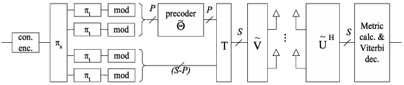
The serial-to-parallel converter organizes the symbol vector $\mathbf{x}$ as $\mathbf{x}=[\mathbf{x}_{\boldsymbol{\eta}}^{T}\,\vdots\,\mathbf{x}_{\boldsymbol{\omega}}^{T}]^{T}=[x_{\eta_{1}}\,\cdots\,x_{\eta_{P}}\vdots$ $\,x_{\omega_{1}}\,\cdots\,x_{\omega_{(S-P)}}]^{T}$, where $\mathbf{x}_{\boldsymbol{\eta}}$ and $\mathbf{x}_{\boldsymbol{\omega}}$ consist of the modulated entries to be transmitted on the subchannels specified in $\boldsymbol{\eta}$ and $\boldsymbol{\omega}$, respectively. The $S\times 1$ detected symbol vector $\mathbf{y}=[\mathbf{y}_{p}^{T}\,\vdots\,\mathbf{y}_{n}^{T}]^{T}=[y_{1}\,\cdots\,y_{P}\,\vdots$ $\,y_{P+1}\,\cdots\,y_{S}]^{T}$ at the receiver is written as

where $\boldsymbol{\Gamma}$ is a block diagonal matrix, $\boldsymbol{\Gamma}=\textrm{diag}[\boldsymbol{\Gamma}_{p},\,\boldsymbol{\Gamma}_{n}]$, with diagonal matrices defined as $\boldsymbol{\Gamma}_{p}=\textrm{diag}[\lambda_{\eta_{1}},$ $\,\cdots,\,\lambda_{\eta_{P}}]$, $\boldsymbol{\Gamma}_{n}=\textrm{diag}[\lambda_{\omega_{1}},\,\cdots,\,\lambda_{\omega_{(S-P)}}]$, and $\mathbf{n}=[\mathbf{n}_{p}^{T}\,\vdots\,\mathbf{n}_{n}^{T}]^{T}$ is an additive white Gaussian noise vector with zero mean and variance $N_{0}=N/SNR$. The matrix $\mathbf{H}$ is complex Gaussian with zero mean and unit variance, and to make the received signal-to-noise ratio $SNR$, the total transmitted power is scaled as $N$. The input-output relation in (3) is decomposed into two equations as

The ML decoding of the detected symbol $\mathbf{\hat{x}}=[\mathbf{\hat{x}}_{\boldsymbol{\eta}}^{T}\,\vdots\,\mathbf{\hat{x}}_{\boldsymbol{\omega}}^{T}]^{T}=[\hat{x}_{\eta_{1}}\,\cdots\,\hat{x}_{\eta_{P}}\,\vdots\,\hat{x}_{\omega_{1}}\,\cdots\,\hat{x}_{\omega_{(S-P)}}]^{T}$ is given by

where $\chi^{S}$ represents the $S$-dimensional product space based on $\chi$. For PPMB, the symbol can be detected in a parallel fashion as

for the precoded symbol, and

for the non-precoded symbol where $\tilde{l}$ is the corresponding index transformed by $\mathbf{T}$.

Fig. 1(b) represents the structure of Bit-Interleaved Coded Multiple Beamforming with Constellation Precoding (BICMB-CP). First, the convolutional encoder with code rate $R_{c}=k_{c}/n_{c}$, possibly combined with a perforation matrix for a high rate punctured code, generates the codeword $\mathbf{c}$ from the information bits. Then, the spatial interleaver $\pi_{s}$ distributes the coded bits into $S$ streams, each of which is interleaved by an independent bit-wise interleaver $\pi_{t}$. The interleaved bits are mapped by Gray encoding onto the symbol sequence $\mathbf{X}=[\mathbf{x}_{1}\,\cdots\,\mathbf{x}_{K}]$, where $\mathbf{x}_{k}$ is an $S\times 1$ symbol vector at the $k^{th}$ time instant. Each entry of $\mathbf{x}_{k}$ belongs to a signal set $\chi$.

The symbol vector $\mathbf{x}_{k}$ is multiplied by the $S\times S$ precoder $\boldsymbol{\Theta}$ in (II-A). When all of the $S$ modulated entries are precoded ($P=S$), we call the resulting system Bit-Interleaved Coded Multiple Beamforming with Full Precoding (BICMB-FP), otherwise, we call it Bit-Interleaved Coded Multiple Beamforming with Partial Precoding (BICMB-PP). The precoded symbol vector is transmitted on the MIMO channel described in Section II-A.

As in UMB-CP, the spatial interleaver arranges the symbol vector $\mathbf{x}_{k}$ as $\mathbf{x}_{k}=[\mathbf{x}_{k,\boldsymbol{\eta}}^{T}\,\vdots\,\mathbf{x}_{k,\boldsymbol{\omega}}^{T}]^{T}=[x_{k,\eta_{1}}$ $\cdots\,x_{k,\eta_{P}}\,\vdots\,x_{k,\omega_{1}}\,\cdots\,x_{k,\omega_{(S-P)}}]^{T}$. The $S\times 1$ detected symbol vector $\mathbf{r}_{k}=[(\mathbf{r}_{k}^{p})^{T}\,\vdots\,(\mathbf{r}_{k}^{n})^{T}]^{T}=[r_{k,1}\,\cdots$ $r_{k,P}\,\vdots\,r_{k,P+1}\,\cdots\,r_{k,S}]^{T}$ at the $k^{th}$ time instant is

where $\mathbf{n}_{k}=[(\mathbf{n}_{k}^{p})^{T}\,\vdots\,(\mathbf{n}_{k}^{n})^{T}]^{T}$ is an additive white Gaussian noise vector.

The location of the coded bit $c_{k^{\prime}}$ within the symbol sequence $\mathbf{X}$ is known as $k^{\prime}\rightarrow(k,l,i)$, where $k$, $l$, and $i$ are the time instant in $\mathbf{X}$, the symbol position in $\mathbf{x}_{k}$, and the bit position on the label $x_{k,l}$, respectively. Let $\chi_{b}^{i}$ denote a subset of $\chi$ whose labels have $b\in\{0,1\}$ in the $i^{th}$ bit position. By using the location information and the input-output relation in (8), the receiver calculates the maximum likelihood bit metrics for the coded bit $c_{k^{\prime}}$ as

where $\xi_{c_{k^{\prime}}}^{l,i}$ is a subset of $\chi^{S}$, defined as

In particular, based on the decomposition of (8) similar to (6) and (7), the bit metrics, equivalent to (9) for partial precoding, are

where $\psi_{b}^{l,i}$ is a subset of $\chi^{P}$, defined as

and $\tilde{l}$ is an entry in $\boldsymbol{\omega}$, corresponding to the subchannel mapped by $\mathbf{T}$. Finally, the ML decoder makes decisions according to the rule

Based on the ML decoding in (5), the upper bound to the instantaneous PEP between the transmitted symbol $\mathbf{x}$ and the detected symbol $\mathbf{\hat{x}}$ is calculated as

Let $\mathbf{d}=\left[d_{1}\,\cdots\,d_{S}\right]^{T}=\mathbf{\Theta}(\mathbf{x}-\mathbf{\hat{x}})$. Then, for FPMB, the average PEP becomes

In [8], we showed that equations in the form of (14) have a closed form upper bound expression. We provide a formal statement below.

Generalizing (13) for PPMB, we get an upper bound to PEP as

where

and $\tilde{d}_{s}$ is the $s^{th}$ element of a vector $\mathbf{\tilde{d}}=$ $\mathbf{\tilde{\Theta}}(\mathbf{x}_{\boldsymbol{\eta}}-\mathbf{\hat{x}}_{\boldsymbol{\eta}})$. Let us assume that the constellation precoding matrix $\mathbf{\tilde{\Theta}}$ meets the condition of FPMB to achieve the full diversity order. Since the expression (16) with (17) has a closed form expression similar to (15) as described in FPMB, the $\delta$ value needs to be obtained from a composite vector with the elements as $|\tilde{d}_{s}|^{2}$ and $|x_{\omega_{s}}-\hat{x}_{\omega_{s}}|^{2}$, to observe the diversity behavior of a given pairwise error. In addition, a different pair can lead to different diversity behavior. Therefore, we need to get the maximum $\delta$ out of all the possible pairwise errors to decide the diversity order of a given PPMB system.

All of the distinct pairs of $\mathbf{x}$ and $\mathbf{\hat{x}}$ are divided into three groups in terms of $\mathbf{x}_{\boldsymbol{\eta}}$, $\mathbf{\hat{x}}_{\boldsymbol{\eta}}$, $\mathbf{x}_{\boldsymbol{\omega}}$, and $\mathbf{\hat{x}}_{\boldsymbol{\omega}}$. The first group includes the pairs that have $\mathbf{x}_{\boldsymbol{\eta}}=\mathbf{\hat{x}}_{\boldsymbol{\eta}}$ but $\mathbf{x}_{\boldsymbol{\omega}}\neq\mathbf{\hat{x}}_{\boldsymbol{\omega}}$, and the second group comprises the pairs satisfying $\mathbf{x}_{\boldsymbol{\eta}}\neq\mathbf{\hat{x}}_{\boldsymbol{\eta}}$ but $\mathbf{x}_{\boldsymbol{\omega}}=\mathbf{\hat{x}}_{\boldsymbol{\omega}}$. Finally, the last group consists of the pairs for which $\mathbf{x}_{\boldsymbol{\eta}}\neq\mathbf{\hat{x}}_{\boldsymbol{\eta}}$ and $\mathbf{x}_{\boldsymbol{\omega}}\neq\mathbf{\hat{x}}_{\boldsymbol{\omega}}$. We will present the method to calculate the maximum $\delta$ for each group, and to find $\delta_{max}$ from the groups.

Since the vector $\mathbf{\tilde{d}}$ is a zero vector for the first group, the first summation of $\kappa$ in (17) is zero, resulting in $\delta$ being equal to the minimum of $\boldsymbol{\omega}$. By considering all of the possible pairs, we easily see that $\omega_{1}\leq\delta\leq\omega_{(S-P)}$. Therefore, the maximum value is $\delta_{1}=\omega_{(S-P)}$ which corresponds to the pair satisfying $x_{s}=\hat{x}_{s}$ for all $s$ except $s=\omega_{(S-P)}$. For any pair in the second group, the term with the first singular value survives in $\kappa$, according to the inherited property of the constellation precoding matrix, i.e., $|\tilde{d}_{1}|^{2}>0$. However, the second summation in $\kappa$ disappears since $\mathbf{x}_{\boldsymbol{\omega}}=\mathbf{\hat{x}}_{\boldsymbol{\omega}}$. Therefore, the maximum value of this group is $\delta_{2}=\eta_{1}$. Now, for the third group, both summations in $\kappa$ exist. Then, $\delta$ is chosen to be the smaller value between the minimum of $\boldsymbol{\omega}$ and $\eta_{1}$. In the same manner as was already given in the analysis of the first group, the maximum of the minimum of $\boldsymbol{\omega}$ is found to be $\omega_{(S-P)}$. Therefore, the maximum $\delta$ for this group is $\delta_{3}=\max\{\eta_{1},\,\omega_{(S-P)}\}$. Finally, $\delta_{max}$ is decided as

Example: We provide the diversity analysis of the $4\times 4$ PPMB system with $S=4$ and $P=2$. In this example, we assume that the precoded symbols are transmitted on the subchannel $1$ and $3$ while the non-precoded symbols are transmitted on the subchannel $2$ and $4$. Then, this configuration gives $\boldsymbol{\eta}=\left[1\,\,3\right]$, and $\boldsymbol{\omega}=\left[2\,\,4\right]$. By following the result in (18), $\delta_{max}$ is equal to $\max\left(1,\,4\right)=4$, leading to the diversity order of $1$. The pairwise errors, satisfying $x_{1}=\hat{x}_{1},x_{2}=\hat{x}_{2},x_{3}=\hat{x}_{3}$, but $x_{4}\neq\hat{x}_{4}$, inflict loss on the diversity order of this system. Table I summarizes the diversity order analysis for all of the possible combinations of the $4\times 4$ PPMB system. We will provide simulation results that verify this analysis in Section VI, specifically in Fig. 4.

We assume that the $d_{H}$ coded bits are interleaved such that they are placed in distinct symbols, where $d_{H}$ denotes the Hamming distance between the transmitted codeword $\mathbf{c}$ and the decoded codeword $\mathbf{\hat{c}}$. Since the bit metrics in (9) are the same for the same coded bits between the pairwise errors, the original PEP is replaced by

where the summation is restricted to the symbols corresponding to the different $d_{H}$ coded bits.

Let us define $\mathbf{\tilde{x}}_{k}$ and $\mathbf{\hat{x}}_{k}$ as

where $\bar{c}_{k^{\prime}}$ is the complement of $c_{k^{\prime}}$ in binary codes. It is easily found that $\mathbf{\tilde{x}}_{k}$ is different from $\mathbf{\hat{x}}_{k}$ since the sets that the $l^{th}$ symbols belong to are disjoint, as can be seen from the definition of $\xi_{c_{k^{\prime}}}^{l,i}$. In the same manner, we see that $\mathbf{x}_{k}$ is different from $\mathbf{\hat{x}}_{k}$. With $\mathbf{\tilde{x}}_{k}$ and $\mathbf{\hat{x}}_{k}$, we get, from (19),

Based on the fact that $\|\mathbf{r}_{k}-\boldsymbol{\Gamma}\boldsymbol{\Theta}\mathbf{x}_{k}\|^{2}\geq\|\mathbf{r}_{k}-\boldsymbol{\Gamma}\boldsymbol{\Theta}\mathbf{\tilde{x}}_{k}\|^{2}$ and the relation in (8), equation (21) is upper-bounded by

where

Since $\beta$ is a zero mean Gaussian random variable with variance $2N_{0}\sum_{k,d_{H}}\|\boldsymbol{\Gamma}\boldsymbol{\Theta}(\mathbf{x}_{k}-\mathbf{\hat{x}}_{k})\|^{2}$, the right hand side of (22) is replaced by the $Q$ function as

The numerator in (23) is rewritten as

where $d_{k,s}$ is the $s^{th}$ entry of the vector $\mathbf{d}_{k}=\boldsymbol{\Theta}(\mathbf{x}_{k}-\mathbf{\hat{x}}_{k})$. Using an upper bound to the $Q$ function, we calculate the average PEP as

According to Theorem 1, we can evaluate the diversity order of a given system by calculating the weight vector whose $s^{th}$ element is $\sum_{k,d_{H}}|d_{k,s}|^{2}$. In particular, if the constellation precoder is designed such that

where $\boldsymbol{\theta}_{1}^{T}$ is the first row vector of the precoding matrix $\boldsymbol{\Theta}$, we see that $\sum_{k,d_{H}}|d_{k,1}|^{2}>0$, resulting in the full diversity order of $NM$. Therefore, (26) is a sufficient condition for the full diversity order of BICMB-FP.

The bit metrics in (II-B) lead to the PEP calculation as

where

and $\sum_{k,d_{H}^{p}}$, $\sum_{k,d_{H}^{n}}$ stand for the summation over the $d_{H}^{p}$ and $d_{H}^{n}$ bit metrics, with $d_{H}^{p}$ and $d_{H}^{n}$ denoting the number of different coded bits between the two pairwise errors residing on the precoded and the non-precoded subchannels specified by $\boldsymbol{\eta}$ and $\boldsymbol{\omega}$, respectively. By using the appropriate system input-output relations, the PEP is written as

where $\hat{\beta}=\beta_{p}+\beta_{n}$,

and

Since $\hat{\beta}$ in (28) is a Gaussian random variable with zero mean and variance $2N_{0}\hat{\kappa}$, the PEP can be expressed in a way similar to (23) with the $Q$-function. In addition, if we define $\sigma$ as

where $\hat{d}_{k,r}$ is the $r^{th}$ entry of the vector $\mathbf{\hat{d}}_{k}=\boldsymbol{\tilde{\Theta}}\left(\mathbf{x}_{k,\boldsymbol{\eta}}-\mathbf{\hat{x}}_{k,\boldsymbol{\eta}}\right)$, and $\alpha_{s}$ is the number of times the $s^{th}$ subchannel is used corresponding to $d_{H}^{n}$ bits under consideration, then we can see that $\sigma\leq\hat{\kappa}$. Finally, the average PEP is calculated as

To determine the diversity order from $\sigma$, we need to find the index indicating the first nonzero element in an ordered composite vector which consists of $\sum_{k,d_{H}^{p}}|\hat{d}_{k,r}|^{2}$ and $\alpha_{\omega_{r}}$ as in Theorem 1. If $d_{H}^{p}=0$, the first summation part of $\sigma$ vanishes. In this case, the first index is

In the other case of $d_{H}^{p}>0$, we see that $\mathbf{x}_{k,\boldsymbol{\eta}}$ and $\mathbf{\hat{x}}_{k,\boldsymbol{\eta}}$ are obviously different for the same reason as in the previous section. If the constellation precoder satisfies the sufficient condition of (26), the term with $\lambda_{\eta_{1}}^{2}$ always exists in $\sigma$. By considering the second term of $\sigma$, we get $\delta$ for the case of $d_{H}^{p}>0$

where $\delta^{\prime}$, if it exists, is obtained in the same way as (31). If, in search of $\delta^{\prime}$, no $s$ satisfying the right hand side of (31) exists, we state $\delta^{\prime}$ does not exist and set $\delta=\eta_{1}$, as in (32).
Example: In this example, we employ $4$-state $1/2$-rate convolutional code with generator polynomials $(5,7)$ in octal representation, in an $N=M=S=3$ system. Two types of spatial interleavers are used to demonstrate the different results of the diversity order. A generalized transfer function of BICMB with the specific spatial interleaver and convolutional code provides the $\alpha$-vectors for all of the pairwise errors, whose element indicates the number of times the stream is used for the erroneous bits [8]. In particular, due to the fact that $d_{H}^{p}=\sum_{r=1}^{P}\alpha_{\eta_{r}}$ and $d_{H}^{n}=\sum_{r=1}^{S-P}\alpha_{\omega_{r}}$ where $\alpha_{s}$ is the $s^{th}$ element of the $\alpha$-vector, the generalized transfer function approach in [8] is also useful in the analysis of BICMB-PP. Hence, we rewrite the transfer functions of the systems from [8], where $a$, $b$, and $c$ are the symbolic representation of the $1^{st},2^{nd},3^{rd}$ streams, respectively. The spatial interleaver used in $\mathcal{T}_{1}$ is a simple rotating switch on $3$ streams. For $\mathcal{T}_{2}$, the $u^{th}$ coded bit is interleaved into the stream $s_{\mathrm{mod}(u-1,18)+1}$ where $s_{1}$ = $\cdots$ = $s_{6}$ = $1$, $s_{7}$ = $\cdots$ = $s_{12}$ = $2$, $s_{13}$ = $\cdots$ = $s_{18}$ = $3$ and $\mathrm{mod}$ is the modulo operation. Each term represents an $\alpha$-vector, and the powers of $a$, $b$, $c$ in this term indicate the elements of the $\alpha$-vector corresponding to that term.

Consider the case $\boldsymbol{\eta}=[1\,2]$. We see that all of the $\alpha$-vectors of $\mathcal{T}_{1}$ have $d_{H}^{p}>0$. Since $\eta_{1}=1$, $\delta$ equals $1$ whether $\delta^{\prime}$ exists or not. In fact, $\delta^{\prime}$ does not exist for the term $Z^{8}a^{5}b^{3}$. Therefore, the $\mathcal{T}_{1}$ BICMB-PP system with $\boldsymbol{\eta}=[1\,2]$ achieves the full diversity order while BICMB without constellation precoding [8], or PPMB without Bit-Interleaved Coded Modulation (BICM) loses the full diversity order [25], [26]. For $\mathcal{T}_{2}$, the $\alpha$-vector $[0\,0\,5]$ gives $d_{H}^{p}=0$, resulting in $\delta=3$. Therefore, the $\mathcal{T}_{2}$ BICMB-PP system with $\boldsymbol{\eta}=[1\,2]$ does not achieve the full diversity order.

The same analysis for $\boldsymbol{\eta}=[1\,3]$ results in the diversity order of $9$, and $[2\,3]$ results in $4$ for the transfer function $\mathcal{T}_{1}$. Similarly, both of $[1\,3]$ and $[2\,3]$ result in the diversity of $4$ for $\mathcal{T}_{2}$. As a consequence, we find that proper selection of the subchannels for precoding, as well as the appropriate pattern of the spatial interleaver, is important to achieve the full diversity order of BICMB-PP. We will present simulation results that verify this analysis in Section VI, in particular, in Fig. 8.

References

- [1] H. Jafarkhani, Space-Time Coding: Theory and Practice. Cambridge University Press, 2005.
- [2] H. Sampath, P. Stoica, and A. Paulraj, “Generalized linear precoder and decoder design for MIMO channels using the weighted MMSE criterion,” IEEE Trans. Commun., vol. 49, no. 12, pp. 2198–2206, December 2001.
- [3] D. P. Palomar, J. M. Cioffi, and M. A. Lagunas, “Joint tx-rx beamforming design for multicarrier MIMO channels: A unified framework for convex optimization,” IEEE Trans. Signal Process., vol. 51, no. 9, pp. 2381–2401, September 2003.
- [4] E. Sengul, E. Akay, and E. Ayanoglu, “Diversity analysis of single and multiple beamforming,” IEEE Trans. Commun., vol. 54, no. 6, pp. 990–993, June 2006.
- [5] L. G. Ordonez, D. P. Palomar, A. Pages-Zamora, and J. R. Fonollosa, “High-SNR analytical performance of spatial multiplexing MIMO systems with CSI,” IEEE Trans. Signal Process., vol. 55, no. 11, pp. 5447–5463, November 2007.
- [6] E. Akay, E. Sengul, and E. Ayanoglu, “Bit interleaved coded multiple beamforming,” IEEE Trans. Commun., vol. 55, no. 9, pp. 1802–1811, September 2007.
- [7] E. Akay, H. J. Park, and E. Ayanoglu, “On bit-interleaved coded multiple beamforming,” 2008, arXiv: 0807.2464. [Online]. Available: http://arxiv.org
- [8] H. J. Park and E. Ayanoglu, “Diversity analysis of bit-interleaved coded multiple beamforming,” in Proc. IEEE ICC ‘09, Dresden, Germany, June 2009.
- [9] H. E. Gamal and M. O. Damen, “Universal space-time coding,” IEEE Trans. Inf. Theory, vol. 49, no. 5, pp. 1097–1119, May 2003.
- [10] Y. Xin, Z. Wang, and G. B. Giannakis, “Space-time diversity systems based on linear constellation precoding,” IEEE Trans. Wireless Commun., vol. 2, no. 2, pp. 294–309, March 2003.
- [11] Z. Liu, Y. Xin, and G. B. Giannakis, “Linear constellation precoding for OFDM with maximum multipath diversity and coding gains,” IEEE Trans. Commun., vol. 51, no. 3, pp. 416–427, March 2003.
- [12] W. Zhang, X.-G. Xia, and P. C. Ching, “High-rate full-diversity space-time-frequency codes for broadband MIMO block-fading channels,” IEEE Trans. Commun., vol. 55, no. 1, pp. 25–34, January 2007.
- [13] N. Gresset and M. Khanfouci, “Precoded BICM design for MIMO transmit beamforming and associated low-complexity algebraic receivers,” in Proc. IEEE Globecom ‘08, New Orleans, LA, November 2008.
- [14] E. Zimmermann, W. Rave, and G. Fettweis, “On the complexity of sphere decoding,” in Proc. Wireless Personal Multimedia Communications (WPMC) ‘04, Abano Terme, Italy, September 2004.
- [15] J. Jaldén and B. Ottersten, “On the complexity of sphere decoding in digital communications,” IEEE Trans. Signal Process., vol. 53, no. 4, pp. 1474–1484, April 2005.
- [16] H. G. Han, S. K. Oh, S. J. Lee, and D. S. Kwon, “Computational complexities of sphere decoding according to initial radius selection schemes and an efficient initial radius reduction scheme,” in Proc. IEEE Globecom ‘05, St. Louis, MO, November 2005, pp. 2354–2358.
- [17] B. Cheng, W. Liu, Z. Yang, and Y. Li, “A new method for initial radius selection of sphere decoding,” in Proc. IEEE ISCC ‘07, Aveiro, Portugal, July 2007, pp. 19–24.
- [18] B. Hassibi and H. Vikalo, “On the sphere-decoding algorithm I. Expected complexity,” IEEE Trans. Signal Process., vol. 53, no. 8, pp. 2806–2818, August 2005.
- [19] W. Zhao and G. B. Giannakis, “Sphere decoding algorithms with improved radius search,” IEEE Trans. Commun., vol. 53, no. 7, pp. 1104–1109, July 2005.
- [20] K.-W. Wong, C.-Y. Tsui, R. S.-K. Cheng, and W.-H. Mow, “A VLSI architecture of a K-Best lattice decoding algorithm for MIMO channels,” in Proc. IEEE ISCAS ‘02, vol. 3, Scottsdale, Arizona, May 2002, pp. 273–276.
- [21] T.-A. Huynh, D.-C. Hoang, M. R. Islam, and J. Kim, “Two-level-search sphere decoding algorithm for MIMO detection,” in Proc. IEEE ISWCS ‘08, Reykjavik, Iceland, October 2008.
- [22] J. Tang, A. H. Tewfik, and K. K. Parhi, “Reduced complexity sphere decoding and application to interfering IEEE 802.15.3a piconets,” in Proc. IEEE ICC ‘04, vol. 5, Paris, France, June 2004.
- [23] L. Azzam and E. Ayanoglu, “Reduced complexity sphere decoding for square QAM via a new lattice representation,” in Proc. IEEE Globecom ‘07, Washington, D.C., November 2007.
- [24] A. Zanella, M. Chiani, and M. Z. Win, “A general framework for the distribution of the eigenvalues of Wishart matrices,” in Proc. IEEE ICC ‘08, May 2008, pp. 1271–1276.
- [25] H. J. Park and E. Ayanoglu, “Constellation precoded beamforming,” in Proc. IEEE Globecom ‘09, Honolulu, HI, November 2009.
- [26] ——, “Constellation precoded beamforming,” 2009, arXiv:0903.4738v1. [Online]. Available: http://arxiv.org
- [27] B. Hassibi and H. Vikalo, “On the expected complexity of integer least-squares problems,” in Proc. IEEE ICASSP ‘02, vol. 2, Orlando, FL, May 2002.