The spacetime has two Killing vectors, $\zeta=\partial_{t}$ and $\chi=\partial_{\phi}$ in terms of the BTZ coordinates written down in Appendix B. We will call the conserved quantities associated with them energy $E$ and angular momentum $q$ respectively. The Killing vectors provide a recipe for writing down the first integrals of motion. In our case, using $\zeta^{\mu}=(1,0,0)$, and $\chi^{\mu}=(0,0,1)$, we can write down the conserved quantities associated with them to be

	$\displaystyle E\equiv-g_{\mu\nu}\zeta^{\mu}u^{\nu}=(r^{2}-r_{+}^{2}-r_{-}^{2})\frac{{\rm d}t}{{\rm d}\lambda}+r_{-}r_{+}\frac{{\rm d}\phi}{{\rm d}\lambda},$		(2.1)
	$\displaystyle q\equiv g_{\mu\nu}\chi^{\mu}u^{\nu}=-r_{-}r_{+}\frac{{\rm d}t}{{\rm d}\lambda}+r^{2}\frac{{\rm d}\phi}{{\rm d}\lambda},\hskip 28.45274pt$		(2.2)

where $u^{\mu}=\frac{{\rm d}x^{\mu}}{{\rm d}\lambda}$ and $\lambda$ is the affine parameter. Inverting these and solving for $\dot{\phi}$ and $\dot{t}$ gives,

	$\displaystyle\frac{{\rm d}t}{{\rm d}\lambda}=\frac{Er^{2}-qr_{-}r_{+}}{(r^{2}-r_{-}^{2})(r^{2}-r_{+}^{2})},\hskip 18.06749pt$		(2.3)
	$\displaystyle\frac{{\rm d}\phi}{{\rm d}\lambda}=\frac{q(r^{2}-r_{-}^{2}-r_{+}^{2})+Er_{-}r_{+}}{(r^{2}-r_{-}^{2})(r^{2}-r_{+}^{2})}.$		(2.4)

To get information from beyond the event horizon what we need are spacelike geodesics because we will be taking correlators between two different asymptotic boundaries [23, 7]. So the (integrated) geodesic equation for our choice of signature is $g_{\mu\nu}u^{\mu}u^{\nu}=1$. Using the above expressions for $\dot{\phi}$ and $\dot{t}$, we arrive at the explicit form,

$$\Big(\frac{{\rm d}r}{{\rm d}\lambda}\Big)^{2}+\frac{2Eqr_{-}r_{+}-q^{2}\big(r_{+}^{2}+r_{-}^{2}\big)}{r^{2}}-\frac{(r^{2}-r_{+}^{2})(r^{2}-r_{-}^{2})}{r^{2}}+q^{2}=E^{2}.$$

(2.5)

First thing we note about this equation is that unlike in the case of the static black hole, there is an unavoidable mixing of $q$ and $E$, so it is not immediately possible to interpret $E$ as the energy of a particle in a potential. But one crucial observation is that if one works with two new linear combinations of the basic variables,

	$\displaystyle E^{\prime}=\frac{Er_{+}-qr_{-}}{\sqrt{r_{+}^{2}-r_{-}^{2}}}$		(2.6)
	$\displaystyle q^{\prime}=\frac{Er_{-}-qr_{+}}{\sqrt{r_{+}^{2}-r_{-}^{2}}}$		(2.7)

the equation can be brought to the form of an energy conservation equation for a particle in a well,

$\displaystyle\frac{r^{2}}{(r^{2}-r_{-}^{2})}\Big(\frac{{\rm d}r}{{\rm d}\lambda}\Big)^{2}+(r^{2}-r_{+}^{2})\Big(\frac{q^{2}}{r^{2}-r_{-}^{2}}-1\big)=E^{2}.$

(2.8)

We have suppressed the primes in the new variables. The form of the potential is precisely what one would get for the static BTZ black hole, if one were to set $r_{-}=0$. This is an indication of many of the things that follow: we will often find that the location $r=r_{-}$ takes the place of the singularity, in the case of the spinning black hole. Clearly, after a minor redefinition of $r$, the equation above can be thought of as particle of energy $E^{2}$ in a potential given by,

$$-V(r)=(r^{2}-r_{+}^{2})\Big(1-\frac{q^{2}}{r^{2}-r_{-}^{2}}\big)$$

(2.9)

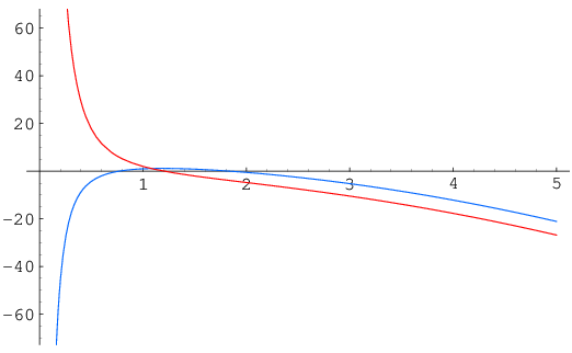
The plot of the potential (in fact $-V$) for some choices of parameters is in fig. 2. When we make the connection between geodesics and correlators, the parameters $E,q$ will often be analytically continued.

The variable redefinition we did in (2.6-2.7) is at the moment merely a matter of convenience. But it becomes much more suggestive when we realize that it follows immediately from a coordinate change of the BTZ metric:

$\displaystyle t^{\prime}=\frac{t-\Omega\phi}{\sqrt{1-\Omega^{2}}},\ \phi^{\prime}=\frac{\phi-\Omega t}{\sqrt{1-\Omega^{2}}}$

(2.10)

where $\Omega\equiv r_{-}/r_{+}$. Under this coordinate transformation, the BTZ coordinates of Appendix B become

$\displaystyle ds^{2}=-(r^{2}-r_{+}^{2})dt^{2}+\frac{r^{2}dr^{2}}{(r^{2}-r_{+}^{2})(r^{2}-r_{-}^{2})}+(r^{2}-r_{-}^{2})d\phi^{2},$

(2.11)

where again we have suppressed primes. We will call these coordinates the new-BTZ coordinates, and we will use them almost exclusively in what follows³³ 3 We use the same notation $(t,r,\phi)$ for both BTZ and new-BTZ coordinates to avoid running out of symbols, but we will be careful enough to emphasize it when we use the former..

A couple of comments are in order. Note that we are going to a frame co-rotating with the outer horizon as far as the $\phi$ coordinate is considered. If we did only the $\phi$-shift, the new $\phi$ will still be periodic at fixed $t$ and this is a standard form for the metric, as is written (for example) in [2]. But together, the $t$ and $\phi$ coordinate changes force a form of the BTZ quotienting (compare with (9.8)) that looks like

$\displaystyle(t,\phi)\sim\Big(t-\frac{2\pi\Omega}{\sqrt{1-\Omega^{2}}},\phi+\frac{2\pi}{\sqrt{1-\Omega^{2}}}\Big).$

(2.12)

It can be checked that there are still no causal pathologies in the $t$ variable: if we were to draw the variables on a cylinder the identification looks roughly like a helix⁴⁴ 4 I thank J. Evslin for a discussion on this.. But the interpretation that a period of $\phi$ represents the horizon (at $r=r_{+}$) is no longer true. In later sections, we will quantize scalar fields in the BTZ background and we will be concerned with high frequency massive modes which can be associated with classical particle propagation (basically (4.22) with $\nu\rightarrow\infty$). This means that the modes are effectively continuous even though there is quantization arising from the periodicity. Note that these coordinates enable us to maximally take advantage of the fact that BTZ is locally $AdS_{3}$.

Another useful observation is that as $r\rightarrow\infty$, the metric takes the usual Poincare patch form of $AdS_{3}$.

We will have more to say about various aspects of this metric in later sections, but for now, we turn to the determination of Killing quantities and geodesics, as we did in the previous subsection. The relevant equations are immediately written down as

	$\displaystyle(r^{2}-r_{+}^{2})\frac{dt}{d\lambda}=E,\ \ (r^{2}-r_{-}^{2})\frac{d\phi}{d\lambda}=q,\hskip 25.29494pt$		(2.13)
	$\displaystyle\frac{r^{2}}{(r^{2}-r_{-}^{2})}\Big(\frac{{\rm d}r}{{\rm d}\lambda}\Big)^{2}+(r^{2}-r_{+}^{2})\Big(\frac{q^{2}}{r^{2}-r_{-}^{2}}-1\big)=E^{2}.$		(2.14)

The last equation was precisely what we got before for the radial geodesic equation, but now we see its origins in terms of the rewritten metric. The first two equations can also be easily seen to be identical to eqns (2.3, 2.4).

Using the above relations, we can define the proper distance $L(E,q)$, the proper time $t(E,q)$ and the proper angular distance $\phi(E,q)$ between the initial and final points of a spacelike geodesic. We will write them down here explicitly for future reference. To obtain $t(E,q)$ and $\phi(E,q)$, we solve for ${\rm d}\lambda$ from (2.5) and plug it into (2.3), (2.4):

	$\displaystyle t(E,q)$	$\displaystyle=$	$\displaystyle 2\int_{r_{c}}^{\infty}\frac{E\ r}{(r^{2}-r_{+}^{2})\sqrt{(r^{2}-r_{-}^{2})}}\frac{{\rm d}r}{\sqrt{E^{2}+(r^{2}-r_{+}^{2})-\frac{q^{2}(r^{2}-r_{+}^{2})}{(r^{2}-r_{-}^{2})}}},$		(2.15)
	$\displaystyle\phi(E,q)$	$\displaystyle=$	$\displaystyle 2\int_{r_{c}}^{\infty}\frac{q\ r}{(r^{2}-r_{-}^{2})^{3/2}}\frac{{\rm d}r}{\sqrt{E^{2}+(r^{2}-r_{+}^{2})-\frac{q^{2}(r^{2}-r_{+}^{2})}{(r^{2}-r_{-}^{2})}}},$		(2.16)

where $r_{c}$ is defined by $V(r_{c})=E^{2}$, and the factor of 2 accounts for the fact that the geodesic comes in from infinity, turns “around” at the turning point $r_{c}$ and then goes to the other asymptotic infinity. To define $L(E,q)$ on the other hand, we choose the affine parameter as the proper length and regularize by subtracting a $\log r$:

$$L(E,q)=2\lim_{r\rightarrow\infty}\Big[\int_{r_{c}}^{r}\frac{r{\rm d}r}{\sqrt{(r^{2}-r_{-}^{2})}\sqrt{E^{2}+(r^{2}-r_{+}^{2})-\frac{q^{2}(r^{2}-r_{+}^{2})}{(r^{2}-r_{-}^{2})}}}-\log r\Big].$$

(2.17)

This regularization is explained (in the closely related context of higher dimensional AdS Schwarzschild black holes) in [13]. We will later explicitly evaluate these integrals.

We will see that with the notion of geodesics defined here, it makes sense to talk about probing the Cauchy horizon from an entangled CFT, in the large-$\nu$ limit that we mentioned. We turn to a heuristic construction that can provide such a dual description next.

We take the geodesics (2.13)-(2.14) as the fundamental objects. It can be seen that these geodesics can probe the inner horizon (we will see this in more detail in section 5). If the spinning black hole has an entangled CFT description, we expect that these geodesics have an interpretation in terms of thermal correlators. Much of what we do in this section is based on heuristic generalizations of the Rindler wedge and on the idea that there should be an entangled description between two halves of the Rindler wedge. In particular, the arguments are meant to motivate, rather than derive our proposal.

There exists a general strategy for constructing thermal (Hartle-Hawking-like) vacua which is based on the fact that the spacetime under consideration has a bifurcate Killing horizon⁵⁵ 5 All spacetimes we discuss have bifurcate Killing horizons. I thank A. Virmani for clarifications on some questions related to them.. The basic idea is that such spacetimes can be mapped to the Rindler wedge where the problem has a well-known solution [29] in terms of Bogolubov transformations. In the large mass-large frequency limit which results in the geodesic approximation, we expect that the quantization of the modes due to the quotienting in (2.11) can be ignored. (We work exclusively with momentum space correlators in this work.) When the quotienting is ignored, the metric (2.11) can be thought of as that of a bifurcate Killing horizon, where $r=r_{+}$ is a bifurcation line (namely, $\phi$-coordinate). The standard strategy now to construct a thermal state is to write down the Kruskal-like coordinates for the metric in (2.11). Then we will interpret the two Rindler halves that arise as the two asymptotic regions corresponding to the entangled CFTs. Using standard Bogolubov transformations, this would give us a construction of the putative vacuum state. We do this in an appendix. Essentially, this ends up giving us a canonical ensemble description of the thermal state⁶⁶ 6 To be more precise, all we need is that our thermal state is one that gives rise to momentum space correlators that reduce to the canonical thermal correlators in the large $\nu$ limit., but note that the energy that one uses in this description is related by a variable redefinition (2.6, 2.7) to the standard notion of energy and (angular) momentum in BTZ.

We emphasize that this construction is a proposal and not a derivation. In particular, there is an order of limits ambiguity associated to ignoring the quotienting in the large-$\nu$ limit. But we will see that the results that one gets from this proposal are reasonable, so we will take this as our working hypothesis for defining thermal correlators for spinning BTZ in the large-$\nu$ limit. Note that effectively, our consruction involves entanglement between two Poincare $AdS_{3}$ patches in an appropriate way.

It is generally believed that spinning black holes should be described by grand canonical ensembles. But in the AdS-CFT context, the interpretation of the situation might be a bit different. We will see in subsection 3.3 that to define a vacuum state for scalar fields which does not get into trouble with super-radiance, we need to quantize with respect to a time coordinate that is timelike everywhere outside the horizon. The time coordinate in a co-rotating (with the horizon) coordinate system is precisely such a coordinate. It seems natural from an AdS/CFT perspective that quantization in such a co-rotating frame (where the the chemical potential $\Omega$ is effectively invisible) should in fact be described in the canonical ensemble. We will make some comments in the final section about the precise interpretation of such a canonical thermal state for rotating black holes. Since our coordinate system is co-rotating, we believe that a natural thermal state to consider is in the canonical ensemble. We will also see later on that when we choose the canonical form, it gives rise to very reasonable matches and interpretations. So it seems that especially in the specific case of BTZ, an appropriate canonical ensemble construction is useful.

The fundamental reason why this works computationally is because of the simple form of the BTZ metric. In fact by defining $\rho=\sqrt{r^{2}-r_{-}^{2}}$, we can bring the spinning BTZ metric (2.11) to the form

$\displaystyle ds^{2}=-(\rho^{2}-R^{2})dt^{2}+\frac{d\rho^{2}}{\rho^{2}-R^{2}}+\rho^{2}d\phi^{2}$

(3.1)

where $R^{2}=r_{+}^{2}-r_{-}^{2}$. This has the same form as that of the non-rotating BTZ metric, except for the fact that $\rho=0$ is classically the Cauchy horizon and not the singularity⁷⁷ 7 Note also the quotienting (2.12).. We are already seeing hints from the geometry that there exists a close analogy between the Cauchy horizon and the static BTZ singularity.

The bottomline is that we take the construction presented in Appendix C as the definition (effective at least in the large $\nu$ limit) of our thermal correlators. This gives rise to the bulk correlator (see (4.1) and Appendix C for notation)

$\displaystyle{\cal G}_{+}(r,r^{\prime};\omega,p)=\frac{1}{2\omega}\frac{e^{\beta\omega}}{e^{\beta\omega}-1}X_{\omega p}(r)X_{\omega p}(r^{\prime})$

(3.2)

Now, using standard Lorentzian[25]-AdS/CFT[24], we can define correlators of boundary operators that are dual scalar fields in the bulk. The real-time thermal correlators between these boundary operators can be defined by taking the bulk correlators in the limit when the insertions go to the boundary. We will deal with boundary Wightman correlators following the conventions of [16]. These can be constructed as

$\displaystyle G_{+}(\omega,p)=\lim_{r\rightarrow\infty}(2\nu r^{\Delta})(2\nu{r^{\prime}}^{\Delta}){\cal G}_{+}(r,r^{\prime};\omega,p)$

(3.3)

where in three dimensions, for a scalar field of mass $m$,

$$\Delta_{\pm}=1\pm\nu,\ \ {\rm with}\ \ \nu=\sqrt{1+m^{2}}.$$

(3.4)

The reason we are interested in the thermal vacuum is because it shows up in a proposal by Maldacena [7] for describing AdS black holes as thermal states using two entangled CFTs. The correlators in the thermal vacuum will be interpreted as correlators in the entangled CFT.

The first step in the Maldacena construction is the observation (made earlier by Israel) that a thermal state can be written as an entangled state. A “thermal state” $|0(\beta,\mu)\rangle$ in the grand canonical ensemble is defined as a state where the relation

$\displaystyle\langle 0(\beta,\Omega)|A|0(\beta,\Omega)\rangle=\frac{1}{Z}{\rm Tr}(e^{-\beta(H-\Omega J)}A)$

(3.5)

holds for any observable $A$. The $\Omega$ acts as the chemical potential for the appropriate charge, $J$. Here $Z$ is the grand-canonical partition function

$\displaystyle Z={\rm Tr}(e^{-\beta(H-\Omega J)}).$

(3.6)

The fact that a state is thermal means that we don’t have a complete description of it, and that our description coarse-grains (i.e., traces) over some degrees of freedom. This is the “entangled” description of a thermal state. The key observation is that (3.5) can be reproduced by explicit computation if we define

$\displaystyle|0(\beta,\Omega)\rangle=\frac{1}{Z[\beta,\Omega]^{\frac{1}{2}}}\sum_{n}e^{-\frac{\beta\,(E_{n}-\Omega J_{n})}{2}}|E_{n},J_{n}\rangle\otimes|E_{n},J_{n}\rangle\,$

(3.7)

if $A$ acts only on one of the Hilbert spaces in the tensor product.

The maximally extended spacetime of a black hole in AdS involves (at least) two boundaries. So it is natural to propose that the entangled state (3.7) between the CFTs living on these two boundaries is precisely the (Hartle-Hawking) thermal state of the black hole [7]. The standard AdS-CFT correspondence allows us to compute CFT Green functions as boundary limits of bulk correlators. So we can compute the Green’s functions in the Hartle-Hawking vacuum, take the limit where the points go to the (same) boundary and get the thermal Green functions in the CFT. If we take the points to go to distinct boundaries then we get thermal correlators where one operator is inserted on one CFT and the other is inserted on the other CFT. These correlators correspond to geodesics that go inside the horizon, and they are what we will use to extract the information we are after.

When the angular momentum $J$ of a black hole becomes non-zero, its conformal structure undergoes a drastic change: in particular, the Penrose diagrams of rotating black holes can be extended infinitely. They involve new asymptotic boundaries, Cauchy horizons, and timelike singularities (instead of the spacelike singularities in the non-rotating case). So in the grand canonical version of the Maldacena prescription outlined above, most of these regions have to be (implicitly) considered fictitious⁸⁸ 8 Note that when the chemical potential is zero, the black hole becomes uncharged and static, and one can work with the canonical ensemble. Because there are only two asymptotic boundaries, things are straightforward.. Note that in our canonical ensemble formulation of the previous subsection, such problems are automatically avoided: we can put the two CFTs on the boundaries of the two Rindler-like half-spaces from the previous subsection. Putting the CFTs on only two boundaries is natural from the above entangled/thermal description, as well as the philosophy that the boundary theory (albeit thermal) is the full definition of the theory. Conversely, we can take such a description as the definition of the theory and aim to see what this view implies for the internal structure of the black hole. At the end of our work, we will find evidence that this is in fact a self-consistent assumption: the regions beyond the Cauchy horizon will in fact be excised from the CFT correlators. This is also what one expects from numerical gravity simulations.

Another reason why it is reasonable to consider only two boundaries seriously in the CFT picture is that much of the motivation for the Maldacena proposal comes from the Hartle-Hawking construction of the wavefunction of the eternal black hole Universe⁹⁹ 9 Not to be confused with the Hartle-Hawking thermal state [34]. The latter is a state defined on the Fock space of fields in the black hole geometry, while the former is a wave-function (in the Wheeler-DeWitt sense) of the spacetime itself. When the backreaction of the scalar on the geometry can be ignored, the only contribution to the full wave function that we will need to keep track of is the scalar part. This is the premise of QFT in curved space.[35]. There, two boundaries are the only possibility. The conclusions of this paper show that the Cauchy horizon looks like a singularity from the boundary theory, so that the Maldacena proposal is indeed self-consistent.

Spinning black holes can exhibit super-radiance which can make the vacuum states defined on them ill-defined [8]. In our construction, we could bypass this problem by going to a new coordinate frame because we are in AdS, but it is instructive to see this in detail. The basic idea behind super-radiance is easy to understand. When a mode of energy $\delta M\sim\hbar\omega$ and angular momentum $\delta J\sim\hbar k$ is incident on a black hole, the hole’s mass and angular momentum change according to $dM/dJ=\omega/k$. This, together with the first law $dM=T_{H}dA+\Omega dJ$ implies that $dM=T_{H}\omega dA/(\omega-k\Omega)$. Since $dA\geq 0$ by the second law, this means that for incident modes that satisfy $\omega<k\Omega$, the hole looses mass. This is the wave-analogue of the Penrose process. The scattered wave has more energy than the incident wave because the hole is loosing its energy to the mode, and this is the phenomenon of super-radiance.

Super-radiance arises because rotating black holes have an ergosphere that stretches outside the outer horizon from where angular momentum can be extracted without falling into the hole. This is because the energy as defined from infinity is with-respect to a time-like Killing vector that is no longer timelike inside the ergosphere. If there exists a globally defined time-like rotational Killing vector that stretches all the way to the boundary of the spacetime, there will not be any super-radiant instabilities. For Kerr black holes in AdS, such an argument was made in [10] for black holes that are not rotating too fast. We will adapt that argument here for the case of BTZ. From the metric presented in (9.7), we can write down an angular velocity at the horizon given by¹⁰¹⁰ 10 See Appendix B for notations. We are working with the usual BTZ coordinates here.

$\displaystyle\Omega=\frac{r_{-}}{r_{+}}.$

(3.8)

Now the co-rotating Killing field is

$\displaystyle\chi=\frac{\partial}{\partial t}+\Omega\frac{\partial}{\partial\phi}.$

(3.9)

It can be checked directly using the metric, that the norm of this vector is given by

$\displaystyle||\chi||^{2}=-\frac{(r^{2}-r_{+})^{2}(r_{+}^{2}-r_{-}^{2})}{r_{+}^{2}}.$

(3.10)

So the vector is everywhere timelike outside the outer horizon. Using this $\chi$ we can repeat the argument presented in section II.B of [10]. This shows that the BTZ spacetime is stable against superradiance, at least away from extremality.

To get a time coordinate which can be used to define positive energy modes, we can set $\chi=\frac{\partial}{\partial T}$. Writing (3.9) as

$\displaystyle\frac{\partial}{\partial T}=\frac{\partial t}{\partial T}\frac{\partial}{\partial t}+\frac{\partial\phi}{\partial T}\frac{\partial}{\partial\phi},$

(3.11)

which implies that the new coordinates $T$ and $\Phi$ have to be defined by

$\displaystyle t=T+f(\Phi),\ \ \ \phi=\Omega T+g(\Phi).$

(3.12)

for arbitrary functions $f$ and $g$. So we see that going to a co-rotating frame with respect to the horizon makes the time coordinate positive definite everywhere outside the horizon. The coordinate transformation (2.10) that leads to (2.11) is one such choice.

That the rotating BTZ black hole is the dominant contribution to the gravity partition function was shown in [22, 9].

In the case of the BTZ black hole, as mentioned in the introduction, the major simplification is that we can solve the scalar field equation in the metric (2.11) exactly. We first separate variables as

$$\varphi=\sum_{n,\omega}\exp(ip\phi)\exp(-i\omega t)X_{\omega,p}(r).$$

(4.1)

The equation of motion $(\Box-m^{2})\varphi=0$ reduces upon defining the lapse function

$$N^{2}=\frac{(r^{2}-r_{+}^{2})(r^{2}-r_{-}^{2})}{r^{2}},$$

(4.2)

to

$$X_{\omega,p}^{\prime\prime}+\frac{(rN^{2})^{\prime}}{rN^{2}}X_{n\omega}^{\prime}+\frac{1}{N^{2}}\Big[\frac{\omega^{2}}{r^{2}-r_{+}^{2}}-\frac{p^{2}}{r^{2}-r_{-}^{2}}-m^{2}\Big]X_{\omega,p}=0.$$

(4.3)

We can bring this to a Schrodinger form (which will be useful when we make the WKB approximation) by defining

$$Y_{\omega,p}(r)=(r^{2}-r_{-}^{2})^{1/4}X_{\omega,p}(r),$$

(4.4)

and the result can be written as

$\displaystyle\frac{d^{2}Y_{\omega,p}}{dz^{2}}+\Big[\omega^{2}-m^{2}(r^{2}-r_{+}^{2})-\frac{p^{2}(r^{2}-r_{+}^{2})}{r^{2}-r_{-}^{2}}-\frac{(3r^{2}+r_{+}^{2}-4r_{-}^{2})(r^{2}-r_{+}^{2})}{r^{2}-r_{-}^{2}}\Big]Y_{\omega,p}=0$

(4.5)

where we have introduced a tortoise coordinate $z$ which is defined in (10.2).

Equation (4.3) is solvable, because the BTZ wave equation is solvable [26, 28]. The wave equation in the standard BTZ coordinates is solved by using a variable redefinition of the form eqn.(57) in [28]. We can use a similar trick here, by defining

$$X_{\omega,p}=(r^{2}-r_{+}^{2})^{\alpha}(r^{2}-r_{-}^{2})^{\beta}Z_{\omega,p}\left(u\equiv\frac{r^{2}-r_{-}^{2}}{r_{+}^{2}-r_{-}^{2}}\right),$$

(4.6)

where $Z_{\omega,p}$ is a new function with a new radial variable $u$ as its argument, and

	$\displaystyle\alpha$	$\displaystyle=$	$\displaystyle i\frac{\omega}{2\sqrt{(r_{+}^{2}-r_{-}^{2})}}$
	$\displaystyle\beta$	$\displaystyle=$	$\displaystyle i\frac{p}{2\sqrt{(r_{+}^{2}-r_{-}^{2})}}.$		(4.7)

Here $u$ lies in the range $1\leq u\leq\infty$ as $r$ ranges between the outer horizon and the boundary. The equation of motion now changes into the hypergeometric form

$$u(1-u)Z_{\omega,p}^{\prime\prime}+\{c-(a+b+1)u\}Z_{\omega,p}^{\prime}-abZ_{\omega,p}=0,$$

(4.8)

where

	$\displaystyle a$	$\displaystyle=$	$\displaystyle\alpha+\beta+\frac{\Delta_{+}}{2}$
	$\displaystyle b$	$\displaystyle=$	$\displaystyle\alpha+\beta+\frac{\Delta_{-}}{2}$		(4.9)
	$\displaystyle c$	$\displaystyle=$	$\displaystyle 2\beta+1,$

with $\Delta_{\pm}$ defined in (3.4).

What we are interested in are solutions that satisfy finiteness-of-energy conditions appropriate for AdS. the nature of solutions depends on whether $\nu$ in (3.4) is integral or not. Since we will be interested in making a large mass-expansion to connect with the geodesic approximation, we will be interested in the large $\nu$-limit, so we can assume that $\nu$ is not an integer.

The general solutions that is well-defined at the boundary $(u\rightarrow\infty)$,

	$\displaystyle Z_{\omega,p}=C_{1}u^{-(\alpha+\beta+h_{+})}F\left(\alpha+\beta+h_{+},\alpha-\beta+h_{+};1+\nu;1/u\right)+\hskip 28.45274pt$
	$\displaystyle\hskip 28.45274pt+C_{2}u^{-(\alpha+\beta+h_{-})}F\left(\alpha-\beta+h_{-},\alpha+\beta+h_{-};1-\nu;1/u\right),$		(4.10)

where $F\equiv{}_{2}F_{1}$ is the hypergeometric function, and $h_{\pm}=\Delta_{\pm}/2$. The radial part $X_{\omega,p}$ is related to the above expression through (4.6),

$$X_{\omega,p}\sim(u-1)^{\alpha}u^{\beta}Z_{\omega,p}.$$

(4.11)

Lets collect the leading behavior of the various coordinates at the boundary and the outer horizon here for convenience:

		$\displaystyle{\rm horizon}\ (r\rightarrow r_{+}):$	$\displaystyle\ \ u\sim 1+\frac{r^{2}-r_{+}^{2}}{r_{+}^{2}-r_{-}^{2}}\rightarrow 1,$		(4.12)
			$\displaystyle\ z\sim-\frac{1}{2\sqrt{(r_{+}^{2}-r_{-}^{2})}}\ln(r^{2}-r_{+}^{2})\rightarrow\infty,\hskip 28.45274pt$
		$\displaystyle{\rm boundary}\ (r\rightarrow\infty):$	$\displaystyle\ \ u\sim\frac{r^{2}}{r_{+}^{2}-r_{-}^{2}}\rightarrow\infty,\ \ z\sim\frac{1}{r}\rightarrow 0.$		(4.13)

With these, we can impose that the solution satisfy the usual AdS-falloff,

$$\phi(r,x)\rightarrow r^{-\Delta_{-}}\phi_{0}(x),$$

(4.14)

(for some $\phi_{0}$) which forces $C_{2}$ to be zero. Using identity (C.17) from [27] we can write

	$\displaystyle X_{\omega,p}$	$\displaystyle=$	$\displaystyle C_{1}(u-1)^{\alpha}u^{-\alpha-h_{+}}F(\alpha+\beta+h_{+},\alpha-\beta+h_{+};1+\nu;1/u)$		(4.15)
		$\displaystyle=$	$\displaystyle C_{1}\big[A(u-1)^{\alpha}u^{\beta}F(h_{+}+\alpha+\beta,h_{-}+\alpha+\beta;1+2\alpha;1-u)+$
			$\displaystyle\hskip 14.22636pt+B(u-1)^{-\alpha}u^{-\beta}F(h_{-}-\alpha-\beta,h_{-}-\alpha-\beta;1-2\alpha;1-u)\big]$

where

	$\displaystyle A=\frac{\Gamma(1+\nu)\Gamma(-2\alpha)}{\Gamma(h_{+}-\alpha-\beta)\Gamma(h_{+}-\alpha+\beta)},$		(4.16)
	$\displaystyle B=\frac{\Gamma(1+\nu)\Gamma(2\alpha)}{\Gamma(\alpha+\beta+h_{+})\Gamma(\alpha-\beta+h_{+})}.$		(4.17)

It turns out that $A=B^{*}$. Using this we can see that at the horizon ($u\rightarrow 1$), the mode $X_{\omega,p}$ reduces to

$\displaystyle X_{\omega,p}\rightarrow C_{1}|Z|\Big(\exp{(-i\delta)}\exp(-i\omega z)+\exp{(i\delta)}\exp(i\omega z)\Big),$

(4.18)

where in the first line we have used the leading behavior of the coordinates to rewrite the expression in terms of $z$. The phase can be completely fixed, but we will not need it. Normalizing $X_{\omega,p}$ at the horizon with $C_{1}|Z|=1$ and using this back in the asymptotic form at the boundary, we find that

$$X_{n\omega}\rightarrow C(\omega,p)(r_{+}^{2}-r_{-}^{2})^{(1+\nu)/2}\ r^{-(1+\nu)},$$

(4.19)

where we have renamed $C_{1}$ as $C(\omega,p)$. Using the definitions of $A$ and $B$, we can explicitly write down $C(\omega,p)$:

$\displaystyle C(\omega,p)^{2}=\frac{\Gamma(h_{+}-\alpha-\beta)\Gamma(h_{+}-\alpha+\beta)\Gamma(h_{+}+\alpha+\beta)\Gamma(h_{+}+\alpha-\beta)}{\Gamma(1+\nu)^{2}\Gamma(2\alpha)\Gamma(-2\alpha)}.$

(4.20)

Using (3.3) we can now compute

	$\displaystyle G_{+}(\omega,p)=\frac{4\nu^{2}}{2\omega}\frac{e^{\beta\omega}}{e^{\beta\omega}-1}(r_{+}^{2}-r_{-}^{2})^{1+\nu}C(\omega,p)^{2}\hskip 86.72377pt$		(4.21)
	$\displaystyle=\frac{\beta(r_{+}^{2}-r_{-}^{2})^{1+\nu}e^{\beta\omega/2}}{2\pi^{2}\Gamma(\nu)^{2}}\Gamma(h_{+}-\alpha-\beta)\Gamma(h_{+}-\alpha+\beta)\Gamma(h_{+}+\alpha+\beta)\Gamma(h_{+}+\alpha-\beta).$

These results reduce to equations (13) and (15) in [18] when the black hole is static (except for some minor errors in [18]).

We can make a connection with the geodesic approximation by setting

$$p=k\nu,\ \ \omega=u\nu,\ \ m^{2}=\nu^{2}-1.$$

(4.22)

The basic idea is that when the mass of the scalar is large (or equivalently, $\nu\rightarrow\infty$), the particle approximation becomes good, and so the boundary-boundary correlator is dominated by contributions from the bulk geodesics that connect the two points. Since the large-mass limit is a semi-classical limit, and the scalar field equation (in the tortoise coordinate) is just a Schrödinger equation with a complicated potential, the first thing we do in order to make a connection with the geodesics is to try a WKB solution for the “wave-function”. Plugging in $Y=e^{\nu S}$, we get to leading order in $1/\nu$

$\displaystyle-(\partial_{z}S)^{2}+V(z)=u^{2}.$

(4.23)

where the potential

$$V(z)=(r^{2}-r_{+}^{2})\Big(1+\frac{k^{2}}{r^{2}-r_{-}^{2}}\Big)$$

(4.24)

will be a crucial object in the rest of this paper. For real $k$, which will be enough for our purposes, the plot takes the form given in figure 2.

Taking advantage of the boundary condition that when the potential is infinite, the wave function is zero, we start in the classically forbidden region ($0<z<z_{c}$, which is the part close to the AdS boundary). Interpreting $u^{2}$ as the energy of the particle in the well, the standard WKB solution takes the form

$$Y_{\omega,p}^{WKB}(z)=\frac{1}{\sqrt{\kappa(z)}}\exp(\nu{\mathcal{Z}}(z))+...,$$

(4.25)

where

$\displaystyle\kappa(z)=\sqrt{V-u^{2}},\ \ \ {\mathcal{Z}}=\int_{z_{c}}^{z}dz^{\prime}\kappa(z^{\prime})$

(4.26)

where the turning point $z_{c}$ is fixed by

$$(r_{c}^{2}-r_{+}^{2})\Big(1+\frac{k^{2}}{r_{c}^{2}-r_{-}^{2}}\Big)=u^{2}.$$

(4.27)

The dots represent higher corrections to the WKB approximation (higher in $1/\nu$). We start with the situation $u^{2},k^{2}>0$ (in which case there is a unique positive root for $r_{c}$) and then analytically continue to probe the regions inside the horizon.

In the classically allowed region, the standard WKB solution takes the form

	$\displaystyle Y^{WKB}_{\omega,p}(z)$	$\displaystyle=$	$\displaystyle\frac{1}{\sqrt{p(z)}}e^{i(\nu W-\frac{\pi}{4})}+cc.+...,\ \ {\rm where}$		(4.28)
	$\displaystyle W(z)$	$\displaystyle=$	$\displaystyle\int_{z_{c}}^{z}dz^{\prime}p(z^{\prime}),\ \ p(z)=\sqrt{u^{2}-V}$		(4.29)

Near the outer horizon, this reduces to

$\displaystyle Y^{WKB}_{\omega,p}(z)=\frac{1}{\sqrt{u}}e^{i(\omega z+phase)}+cc.$

(4.30)

Comparing to (4.18, 4.4), we fix the relative normalizations as

$\displaystyle Y^{WKB}_{\omega,p}(z)=\frac{Y(z)}{\sqrt{u}(r_{+}^{2}-r_{-}^{2})^{1/4}}$

(4.31)

Using these we find that the boundary Wightman correlator (3.3) in the WKB limit takes the form

	$\displaystyle G_{+}(\omega,p)=\lim_{r,r^{\prime}\rightarrow\infty}\frac{(2\nu)^{2}}{2\nu u}(rr^{\prime})^{1+\nu}\times u\ (r_{+}^{2}-r_{-}^{2})^{1/2}(rr^{\prime})^{-1/2}Y^{WKB}_{\omega,p}(r)Y^{WKB}_{\omega,p}(r^{\prime})$
	$\displaystyle=\lim_{r\rightarrow\infty}2\nu\sqrt{r_{+}^{2}-r_{-}^{2}}\frac{(e^{\nu{\mathcal{Z}}})^{2}}{(\sqrt{r})^{2}}r^{2\nu+1}\ =\ 2\nu\sqrt{r_{+}^{2}-r_{-}^{2}}e^{\nu Z(u,k)},\hskip 72.26999pt$		(4.32)

where $Z$ can be defined in terms of $z$ by

$$Z=2\lim_{z\rightarrow 0}\Big(\int_{z_{c}}^{z}dz^{\prime}\kappa(z^{\prime})-\log z\Big)$$

(4.33)

This $Z$ can be directly related to the geodesic integrals of section 2. To see this note that ${\mathcal{Z}}$ satisfies

$$\Big(\frac{d{\mathcal{Z}}}{dz}\Big)^{2}+(r^{2}-r_{+}^{2})\Big(\frac{-k^{2}}{r^{2}-r_{-}^{2}}-1\Big)=-u^{2}.$$

(4.34)

This is precisely the geodesic equation (2.8), if we make the identification

$$\frac{{\rm d}{\mathcal{Z}}}{{\rm d}z}=-\frac{(r^{2}-r_{-}^{2})^{1/2}}{r}\ \frac{{\rm d}r}{{\rm d}\lambda},\ \ u=iE,\ \ k=iq.$$

(4.35)

The upshot of all this is that we now have a prescription for associating a geodesic with a given Green function determined by $Z(u,k)$: namely, for a given $Z(u,k)$, we can associate a complex geodesic that starts and ends at $r=+\infty$, and with the integrals of motion, $E=-iu$ and $q=-ik$. To fully fix this identification, we also have to specify an analytic continuation because we are starting with real geodesics. The analytic continuation will be discussed later: in the BTZ case it is straightforward because we also know the exact solution.

Directly integrating (4.34), we can write a useful expression for $Z$:

	$\displaystyle Z(u,k)$	$\displaystyle=$	$\displaystyle 2\lim_{r\rightarrow\infty}({\mathcal{Z}}+\log r)=2\lim_{r\rightarrow\infty}\Big(\int_{z(r_{c})}^{z(r)}\frac{{\rm d}{\mathcal{Z}}}{{\rm d}z}{\rm d}z+\log r\Big)$		(4.36)
		$\displaystyle=$	$\displaystyle 2\lim_{r\rightarrow\infty}\Big(\int_{r_{c}}^{r}\frac{r{\rm d}r}{(r^{2}-r_{+}^{2})\sqrt{r^{2}-r_{-}^{2}}}\sqrt{(r^{2}-r_{+}^{2})\Big(1+\frac{k^{2}}{r^{2}-r_{-}^{2}}\Big)-u^{2}}+\log r\Big)$
		$\displaystyle=$	$\displaystyle-L(E,q)-Et(E,q)+q\phi(E,q),$

where in the last line, we have used the identification (4.35) and the equations from section 2. This relation is a consequence of the correlator-geodesic connection. In passing, we mention that we can interpret $L$ and $Z$ as Legendre transforms of each other, with

$$\frac{\partial Z}{\partial E}=-t(E,q),\ \frac{\partial Z}{\partial q}=\phi(E,q).$$

(4.37)

It is possible to relate the geodesic approximation to a saddle point evaluation of the coordinate space correlators, but we will not do so here.

To complete the definition of $Z(u,k)$ of last section, we need to specify an analytic continuation, both for the turning point $r_{c}(u,k)$ and the integration contour. The turning point is fixed by the condition

$$V(r_{c})\equiv(r_{c}^{2}-r_{+}^{2})\Big(1+\frac{k^{2}}{r_{c}^{2}-r_{-}^{2}}\Big)=u^{2}$$

(5.1)

The positive root is

	$\displaystyle r_{c}^{2}(u,k)$	$\displaystyle=$	$\displaystyle\frac{1}{2}(u^{2}-k^{2}+r_{+}^{2}+r_{-}^{2}\pm\sqrt{k^{4}+2k^{2}(r_{+}^{2}-r_{-}^{2}-u^{2})+(r_{+}^{2}-r_{-}^{2}+u^{2})^{2}}),$		(5.2)
		$\displaystyle\equiv$	$\displaystyle\frac{1}{2}(u^{2}-k^{2}+r_{+}^{2}+r_{-}^{2}\pm\sqrt{\Delta}),$

where we have defined a discriminant in the last line. To fully prescribe the analytic continuation, we need to fix the branch cuts. This can be done with the explicit form form of the Green function $G_{+}(\omega,p)$ from (4.21). It is easy to see that there is a line of poles coming from the Gamma functions, which collapse to branch cuts in the large $\nu$ limit:

$$\pm iu\pm ik=\sqrt{r_{+}^{2}-r_{-}^{2}}\Big(\frac{2n}{\nu}+1\Big).$$

(5.3)

A plot of the analyticity struture in $u$-plane is shown in the figure.

With this pole structure (for $k^{2}>0$) its clear that we should do the analytic continuation in $u$ around the origin. One can set the discriminant to zero and find the branch points,

$$u=\pm k\pm i\sqrt{r_{+}^{2}-r_{-}^{2}},$$

(5.4)

(all combinations of signs allowed) and they agree with beginnings of the branch cuts in the figure.

The physics of the situation is clear from the plot of the potential $U\equiv-V$ (plotted against $r$ this time) shown in figure 4. The analogy is to that of a a one-dimensional particle of energy $E^{2}=-u^{2}$ moving in a potential $-V$. The turning point gets inside the outer horizon as $u^{2}$ goes from positive to negative, i.e, imaginary $u$ can probe inside the outer horizon. Also, we see that for $k^{2}>0$, there is an infinite wall at $r=r_{-}$, so that no probe can get past it¹¹¹¹ 11 Note that we have translated the problem to a classical inverse scattering problem..

Note that these statements are true for non-vanishing $k$. When $k=0$, the potential actually reduce to a flipped quadratic, and has a finite intercept on the vertical axis, meaning that for sufficiently negative $u^{2}$, one can reach $r_{-}$. But the problem is that in this case the analytic continuation that we define is not very well-defined, because the branch cuts in the u-plane (figure 3) collapse onto the imaginary axis. So we will not consider this non-generic situation in what follows. This is the caveat that was mentioned in a footnote in the introduction, and is an indication of the fact that BTZ oversimplifies the problem somewhat. A similar issue arises for static BTZ when zero-angular momentum geodesics are used as probes. In the case of the non-rotating $AdS_{5}$ black hole considered by Festuccia and Liu [16], the branch cuts were not parallel to the imaginary axis, so setting $k=0$ was an acceptable simplification. In any event, in the generic case, we find that the turning point tends to the Cauchy horizon as $u\rightarrow\pm i\infty$. It should be emphasized that if one works with the usual BTZ coordinates, none of these interpretations are obvious because of a mixing of variables, and the associated lack of a clean physical picture.

Since the $u$ and $k$ variables we are working with here are rotated versions of the usual BTZ energy and (angular) momentum. The “effective” Penrose diagram of the metric (2.11) is that of a square, and in this picture, these geodesics are approximately null except for the region where they turn back at the Cauchy horizon. In effect what we are doing is to take the geodesic approximation arising from the correlator construction as the “correct” definition of the geometry. This means that the Penrose diagram of the standard rotating BTZ black hole is effectively modified. Note that spacelike/null geodesics from the boundary can never reach the Cauchy horizon and return back in the standard Penrose diagram of the spinning BTZ black hole, figure 7.

Another important point about this potential is that since it is monotonic, it does not allow any (classically) bound geodesics as solutions. One way to check this is to set

$\displaystyle\frac{dV}{dr}=0,\ \frac{d^{2}V}{dr^{2}}=0,$

(5.5)

since as we tune the parameter values, at the onset of a trough in the potential there will be a point of inflection. The potential presented here does not admit simultaneous solutions for these conditions. But we note that for large values of $q$ the potential does get flatter and flatter after a steep fall, even though not quite to zero-slope. These are classically quasi-stationary paths: that is, they do decay classically (and not just by tunneling), but they do so very slowly.

In the absence of bound geodesics BTZ is different from higher dimensional AdS black holes. There, for large enough values of $k$, it is possible to have geodesics stuck in semi-classical equilibrium around the hole as discussed in [32]. But note that the signatures of the singularity/Cauchy horizon is already visible for small $k$, so this is not a problem for our purposes.

In this section, we finally put together all the ingredients and compute the correlators in the limit that they probe the Cauchy horizon. We already know from the previous subsection that $u$ going to $\pm i\infty$ is the limit where the correlators capture the Cauchy horizon. We can first compute the large-$\nu$ limit of the exact correlator (4.21)¹²¹² 12 This limit can also be computed using the geodesic approximation., and then let $u$ go to infinity along the imaginary axis. In doing the computations of this section, we use various Sterling-like asymptotic approximations of Gamma functions along various directions in the complex plane [32, 33].

$G_{+}$ reduces in the large-$\nu$ limit to

$\displaystyle G_{+}(\omega,p)=2\nu\sqrt{r_{+}^{2}-r_{-}^{2}}\ e^{\nu Z^{\prime}}+...,$

(5.6)

where

$\displaystyle Z^{\prime}=\frac{\beta u}{2}+A_{+}\log A_{+}+A_{-}\log A_{-}+\tilde{A}_{+}\log\tilde{A}_{+}+\tilde{A}_{-}\log\tilde{A}_{-}+\log(r_{+}^{2}-r_{-}^{2}).$

(5.7)

We have defined (in analogy with [16]),

$\displaystyle A_{\pm}=\frac{1}{2}\pm\frac{i(u+k)}{2\sqrt{r_{+}^{2}-r_{-}^{2}}},\ \ \tilde{A}_{\pm}=\frac{1}{2}\pm\frac{i(u-k)}{2\sqrt{r_{+}^{2}-r_{-}^{2}}}$

(5.8)

A useful fact in many of the manipulations is that $A_{+}+A_{-}+\tilde{A}_{+}+\tilde{A}_{-}=2$. The geodesic-correlator connection tells us that $Z^{\prime}$ should be equal to $Z=-Et+q\Phi-L$, once one sets $E=-iu,q=-ik$ in the latter. $Z$ can be computed by evaluating the integrals of section 2 explicitly. The result (in terms of $u,k$ is)

	$\displaystyle L(u,k)$	$\displaystyle=$	$\displaystyle-\frac{1}{2}\log(A_{+}A_{-}\tilde{A}_{+}\tilde{A}_{-})-\log(r_{+}^{2}-r_{-}^{2})$		(5.9)
	$\displaystyle t(u,k)$	$\displaystyle=$	$\displaystyle\frac{1}{2}\log\Big(\frac{A_{+}\tilde{A}_{+}}{A_{-}\tilde{A}_{-}}\Big)-i\frac{\beta}{2}$		(5.10)
	$\displaystyle\Phi(u,k)$	$\displaystyle=$	$\displaystyle-\frac{1}{2}\log\Big(\frac{A_{+}\tilde{A}_{-}}{A_{-}\tilde{A}_{+}}\Big)$		(5.11)

which correctly reproduces the expression for $Z^{\prime}$.

References

- [1] R. Penrose, in “Batelle Rencontres,” eds. C. De Witt and J. Wheeler (W. A. Bejamin, 1968). S. Chandrasekhar and J. B. Hartle, “On crossing the Cauchy horizon of a Reissner-Nordstroem black-hole,” Royal Society of London Proceedings Series A, 384, 301 (1982). E. Poisson and W. Israel, “Internal structure of black holes,” Phys. Rev. D 41, 1796 (1990). R. A. Matzner, N. Zamorano and V. D. Sandberg, “Instability of the Cauchy horizon of Reissner-Nordström black holes,” Phys. Rev. D 19, 2821 (1979). C. M. Chambers and I. G. Moss, “Stability of the Cauchy horizon in Kerr-de Sitter space-times,” Class. Quant. Grav. 11, 1035 (1994) [arXiv:gr-qc/9404015].
- [2] V. Balasubramanian and T. S. Levi, “Beyond the veil: Inner horizon instability and holography,” Phys. Rev. D 70, 106005 (2004) [arXiv:hep-th/0405048].
- [3] P. R. Brady and C. M. Chambers, “Nonlinear instability of Kerr type Cauchy horizons,” Phys. Rev. D 51, 4177 (1995) [arXiv:gr-qc/9501025].
- [4] C. J. S. Clarke, “The Analysis of space-time singularities,” Cambridge (1993).
- [5] P. R. Brady, I. G. Moss and R. C. Myers, “Cosmic Censorship: As Strong As Ever,” Phys. Rev. Lett. 80, 3432 (1998) [arXiv:gr-qc/9801032]. W. S. German and I. G. Moss, “Cauchy horizon stability and cosmic censorship,” Phys. Rev. D 66, 010001 (2002) arXiv:gr-qc/0103080.
- [6] E. Witten, “Anti-de Sitter space, thermal phase transition, and confinement in gauge theories,” Adv. Theor. Math. Phys. 2, 505 (1998) [arXiv:hep-th/9803131].
- [7] J. M. Maldacena, “Eternal black holes in Anti-de-Sitter,” JHEP 0304, 021 (2003) [arXiv:hep-th/0106112].
- [8] B. S. Kay and R. M. Wald, “Theorems on the Uniqueness and Thermal Properties of Stationary, Nonsingular, Quasifree States on Space-Times with a Bifurcate Killing Horizon,” Phys. Rept. 207, 49 (1991).
- [9] S. W. Hawking, C. J. Hunter and M. Taylor, “Rotation and the AdS/CFT correspondence,” Phys. Rev. D 59, 064005 (1999) [arXiv:hep-th/9811056].
- [10] S. W. Hawking and H. S. Reall, “Charged and rotating AdS black holes and their CFT duals,” Phys. Rev. D 61, 024014 (2000) [arXiv:hep-th/9908109].
- [11] S. Hemming, E. Keski-Vakkuri and P. Kraus, “Strings in the extended BTZ spacetime,” JHEP 0210, 006 (2002) [arXiv:hep-th/0208003].
- [12] P. Kraus, H. Ooguri and S. Shenker, “Inside the horizon with AdS/CFT,” Phys. Rev. D 67, 124022 (2003) [arXiv:hep-th/0212277].
- [13] L. Fidkowski, V. Hubeny, M. Kleban and S. Shenker, “The black hole singularity in AdS/CFT,” JHEP 0402, 014 (2004) [arXiv:hep-th/0306170].
- [14] T. S. Levi and S. F. Ross, “Holography beyond the horizon and cosmic censorship,” Phys. Rev. D 68, 044005 (2003) [arXiv:hep-th/0304150].
- [15] D. Brecher, J. He and M. Rozali, “On charged black holes in anti-de Sitter space,” JHEP 0504, 004 (2005) [arXiv:hep-th/0410214].
- [16] G. Festuccia and H. Liu, “Excursions beyond the horizon: Black hole singularities in Yang-Mills theories. I,” JHEP 0604, 044 (2006) [arXiv:hep-th/0506202].
- [17] J. Hammersley, “Extracting the bulk metric from boundary information in asymptotically AdS spacetimes,” arXiv:hep-th/0609202. G. Festuccia and H. Liu, “The arrow of time, black holes, and quantum mixing of large N Yang-Mills theories,” arXiv:hep-th/0611098. V. E. Hubeny, H. Liu and M. Rangamani, “Bulk-cone singularities & signatures of horizon formation in AdS/CFT,” arXiv:hep-th/0610041. M. Rangamani and S. F. Ross, “Winding tachyons in BTZ,” arXiv:0706.0663 [hep-th]. A. Hamilton, D. Kabat, G. Lifschytz and D. A. Lowe, “Local bulk operators in AdS/CFT and the fate of the BTZ singularity,” arXiv:0710.4334 [hep-th].
- [18] C. Yang, “Singularities, geodesics and Green functions in the BTZ black hole,” arXiv:hep-th/0611049.
- [19] M. Banados, C. Teitelboim and J. Zanelli, “The Black hole in three-dimensional space-time,” Phys. Rev. Lett. 69, 1849 (1992) [arXiv:hep-th/9204099].
- [20] M. Banados, M. Henneaux, C. Teitelboim and J. Zanelli, “Geometry of the (2+1) black hole,” Phys. Rev. D 48, 1506 (1993) [arXiv:gr-qc/9302012].
- [21] S. Carlip, “The (2+1)-dimensional black hole,” [arXiv:gr-qc/9506079]
- [22] J. M. Maldacena and A. Strominger, “AdS(3) black holes and a stringy exclusion principle,” JHEP 9812, 005 (1998) [arXiv:hep-th/9804085].
- [23] W. Israel, “Thermo field dynamics of black holes,” Phys. Lett. A 57, 107 (1976).
- [24] J. M. Maldacena, “The large N limit of superconformal field theories and supergravity,” Adv. Theor. Math. Phys. 2, 231 (1998) [Int. J. Theor. Phys. 38, 1113 (1999)] [arXiv:hep-th/9711200]. S. S. Gubser, I. R. Klebanov and A. M. Polyakov, “Gauge theory correlators from non-critical string theory,” Phys. Lett. B 428, 105 (1998) [arXiv:hep-th/9802109]. E. Witten, “Anti-de Sitter space and holography,” Adv. Theor. Math. Phys. 2, 253 (1998) [arXiv:hep-th/9802150].
- [25] V. Balasubramanian, P. Kraus and A. E. Lawrence, “Bulk vs. boundary dynamics in anti-de Sitter spacetime,” Phys. Rev. D 59, 046003 (1999) [arXiv:hep-th/9805171]. V. Balasubramanian, P. Kraus, A. E. Lawrence and S. P. Trivedi, “Holographic probes of anti-de Sitter space-times,” Phys. Rev. D 59, 104021 (1999) [arXiv:hep-th/9808017]. I. R. Klebanov and E. Witten, “AdS/CFT correspondence and symmetry breaking,” Nucl. Phys. B 556, 89 (1999) [arXiv:hep-th/9905104].
- [26] I. Ichinose and Y. Satoh, “Entropies Of Scalar Fields On Three-Dimensional Black Holes,” Nucl. Phys. B 447, 340 (1995) [arXiv:hep-th/9412144].
- [27] C. Krishnan, C. Maccaferri and H. Singh, JHEP 0905, 114 (2009) [arXiv:0902.0290 [hep-th]].
- [28] E. Keski-Vakkuri, “Bulk and boundary dynamics in BTZ black holes,” Phys. Rev. D 59, 104001 (1999) [arXiv:hep-th/9808037].
- [29] N. D. Birrell and P. C. W. Davies, “Quantum Fields in Curved Space,” Cambridge (1999).
- [30] S. F. Ross, “Black hole thermodynamics,” arXiv:hep-th/0502195.
- [31] R. M. Wald, “Quantum field theory in curved space-time and black hole thermodynamics,” Chicago, USA: Univ. Pr. (1994) 205 p
- [32] G. Festuccia and H. Liu, “Excursions beyond the horizon: Black hole singularities in Yang-Mills theories”.
- [33] M. V. Berry, “Infinitely many Stokes smoothings in the Gamma function,” Proc. Roy. Soc. Lond. A 434, 465 (1991).
- [34] J. B. Hartle and S. W. Hawking, “Path Integral Derivation Of Black Hole Radiance,” Phys. Rev. D 13, 2188 (1976).
- [35] J. B. Hartle and S. W. Hawking, “Wave Function Of The Universe,” Phys. Rev. D 28, 2960 (1983).
- [36] G. Festuccia and H. Liu, “A Bohr-Sommerfeld quantization formula for quasinormal frequencies of AdS black holes,” arXiv:0811.1033 [gr-qc].
- [37] V. P. Frolov and K. S. Thorne, “RENORMALIZED STRESS - ENERGY TENSOR NEAR THE HORIZON OF A SLOWLY EVOLVING, ROTATING BLACK HOLE,” Phys. Rev. D 39, 2125 (1989).
- [38] R. Emparan and H. S. Reall, “A rotating black ring in five dimensions,” Phys. Rev. Lett. 88, 101101 (2002) [arXiv:hep-th/0110260]. A. A. Pomeransky and R. A. Sen’kov, “Black ring with two angular momenta,” arXiv:hep-th/0612005. H. Elvang and P. Figueras, “Black Saturn,” JHEP 0705, 050 (2007) [arXiv:hep-th/0701035]. J. Evslin and C. Krishnan, “Metastable Black Saturns,” JHEP 0809, 003 (2008) [arXiv:0804.4575 [hep-th]]. H. Iguchi and T. Mishima, “Black di-ring and infinite nonuniqueness,” Phys. Rev. D 75, 064018 (2007) [Erratum-ibid. D 78, 069903 (2008)] [arXiv:hep-th/0701043]. J. Evslin and C. Krishnan, “The Black Di-Ring: An Inverse Scattering Construction,” Class. Quant. Grav. 26, 125018 (2009) [arXiv:0706.1231 [hep-th]]. K. Izumi, “Orthogonal black di-ring solution,” Prog. Theor. Phys. 119, 757 (2008) [arXiv:0712.0902 [hep-th]]. H. Elvang and M. J. Rodriguez, “Bicycling Black Rings,” JHEP 0804, 045 (2008) [arXiv:0712.2425 [hep-th]]. R. Emparan and H. S. Reall, “Black Holes in Higher Dimensions,” Living Rev. Rel. 11, 6 (2008) [arXiv:0801.3471 [hep-th]].
- [39] M. Guica, T. Hartman, W. Song and A. Strominger, “The Kerr/CFT Correspondence,” arXiv:0809.4266 [hep-th]. C. Krishnan and S. Kuperstein, “A Comment on Kerr-CFT and Wald Entropy,” Phys. Lett. B 677, 326 (2009) [arXiv:0903.2169 [hep-th]]. T. Azeyanagi, G. Compere, N. Ogawa, Y. Tachikawa and S. Terashima, “Higher-Derivative Corrections to the Asymptotic Virasoro Symmetry of 4d Extremal Black Holes,” arXiv:0903.4176 [hep-th].
- [40] P. K. Townsend, “Black holes,” arXiv:gr-qc/9707012. S. W. Hawking and G. F. R. Ellis, “The Large scale structure of space-time,” Cambridge University Press, Cambridge, 1973