Fast Arc-Annotated Subsequence Matching in Linear SpaceThanks: An extended abstract of this paper appeared in proceedings of the 36th International Conference on Current Trends in Theory and Practice of Computer Science.
Abstract
An arc-annotated string is a string of characters, called bases, augmented with a set of pairs, called arcs, each connecting two bases. Given arc-annotated strings and the arc-preserving subsequence problem is to determine if can be obtained from by deleting bases from . Whenever a base is deleted any arc with an endpoint in that base is also deleted. Arc-annotated strings where the arcs are “nested” are a natural model of RNA molecules that captures both the primary and secondary structure of these. The arc-preserving subsequence problem for nested arc-annotated strings is basic primitive for investigating the function of RNA molecules. Gramm et al. [ACM Trans. Algorithms 2006] gave an algorithm for this problem using time and space, where and are the lengths of and , respectively. In this paper we present a new algorithm using time and space, thereby matching the previous time bound while significantly reducing the space from a quadratic term to linear. This is essential to process large RNA molecules where the space is likely to be a bottleneck. To obtain our result we introduce several novel ideas which may be of independent interest for related problems on arc-annotated strings.
1 Introduction
An arc-annotated string is a string augmented with an arc set . Each character in is called a base and the arc set is a set of pairs of positions in connecting two distinct bases. We say that is a nested arc-annotated string if no two arcs in share an endpoint and no two arcs cross each other, i.e., for all we have that iff . Given arc-annotated strings and we say that is a arc-preserving subsequence (APS) of , denoted , if can be obtained from by deleting or more bases from . Whenever a base is deleted any arc with an endpoint in that base is also deleted. The arc-preserving subsequence problem (APS) is to determine if . If and are both nested arc-annotated strings we refer to the problem as the nested arc-preserving subsequence problem (NAPS). Fig. 1(a) shows an example of nested arc-annotated strings.

Ribonucleic acid (RNA) molecules are often modeled as nested arc-annotated strings. Here, the string consists of bases from the -letter alphabet , called the primary structure, and an arc set consisting of pairings between bases, called the secondary structure. The secondary structure of RNA is central for many biological functions and it is more preserved in evolution than the primary structure [16, 21, 15, 12, 2, 8]. NAPS is a simple primitive for comparing the secondary structure of the RNA molecules. Furthermore, it may also serve as the subroutine in algorithms for the more general longest common arc-preserving subsequence problem (LAPCS), see Gramm et al. [13].
Building on earlier work in a related model of RNA molecules by Vialette [22], Gramm et al. [13] introduced and gave an algorithm for NAPS using time and space, where and are the lengths of and , respectively. Kida [17] presented an experimental study of this algorithm and Damaschke [10] considered a special restricted case of the problem.
1.1 Results
We assume a standard unit-cost RAM model with word size and a standard instruction set including arithmetic operations, bitwise boolean operations, and shifts. The space complexity is the number of words used by the algorithm. All of the previous results are in same model of computation. Throughout the paper and are nested arc-annotated strings of lengths and , respectively. In this paper we present a new algorithm with the following complexities.
Theorem 1
Given nested arc-annotated strings and of lengths and , respectively, we can solve the nested arc-preserving subsequence problem in time and space .
Hence, we match the running time of the currently fastest known algorithm and at the same time we improve the space from to . This space improvement is critical for processing large RNA molecules. In particular, an algorithm using space quickly becomes infeasible, even for moderate sizes of RNA molecules, due to costly accesses to external memory. An algorithm using space is much more scalable and allows us to handle significantly larger RNA molecules. Furthermore, we note that obtaining an algorithm using time and space is mentioned as an open problem in Gramm et al. [13].
Compared to the previous work by Gramm et al. [13] our algorithm is not only more space-efficient but also simpler. Our algorithm is based on a single unified dynamic programming recurrence, whereas the algorithm by Gramm et al. requires computing and tabulating auxiliary information in multiple phases mixed with dynamic programming. Our approach allows us to better expose the features of NAPS and is essential for obtaining a linear space algorithm.
1.2 Techniques
As mentioned above, our algorithm is based on a new dynamic programming recurrence. Essentially, the recursion expresses for any pair of substrings and of and , respectively, the longest prefix of which is an arc-preserving subsequence of in term of smaller substrings of and . We combine several new ideas with well-known techniques to convert our recurrence into an efficient algorithm.
First, we organize the dynamic programming recurrence into sequences. A sequence for a given substring of is a simple space representation of the longest arc-preserving subsequences of each prefix of in . We show how to efficiently manipulate sequences to get new sequences using a small set of simple operations, called the primitive operations. Secondly, we organize the computation of sequences using a recursive algorithm that traverses the tree structure of the arcs in . The algorithm computes the sequence for each arc in using the primitive operations. To avoid storing too many sequences during the traversal we direct the computation according to the well-known heavy-path decomposition of the tree. This leads to an algorithm that stores at most sequences. Since each sequence uses space the total space becomes .
Finally, to achieve linear space we exploit a structural property of sequences to compress them efficiently. We obtain a new representation of sequences that only requires bits. Plugging in the new representation into our algorithm the total space becomes as desired. However, the resulting algorithm requires many costly compressions and decompressions of sequences at each arc in the traversal. As a practical and more elegant solution we show how to augment the compressed representation of sequences using standard rank/select indices to obtain constant time random access to elements in sequences. This allows us to compress each sequence only once and avoid decompression entirely without affecting the complexity of the algorithm.
1.3 Related Work
Arc-annotated strings are a natural model of RNA molecules that captures both the primary and secondary structure of these. Consequently, a wide range of pattern matching problems for them have been studied, see e.g., [11, 4, 19, 1, 7, 13, 3]. Among these, NAPS is one of the most basic problems.
The NAPS problem generalizes the tree inclusion problem for ordered trees [9, 18, 5]. Here, the goal is to determine if a tree can be obtained from another tree by deleting nodes. This is equivalent to NAPS where all bases in both strings have an incident arc. The authors have shown how to solve the tree inclusion problem in time and space [5]. Compared to our current result for NAPS the space complexity is the same but the time complexity for tree inclusion is a factor better for most values of and . Though our obtained complexities for the tree inclusion problem and NAPS are very similar, the ideas and techniques behind the results differ significantly. While the definition of the two problems seems very similar it appears that the more general NAPS is significantly more complicated. We leave it as an interesting research direction to determine the precise relationship between NAPS and the tree inclusion problem.
1.4 Outline
2 Preliminaries and Notation
Let be an arc-annotated string with arc set . The length of is the number of bases in and is denoted . We will assume that our input strings and have the arcs and , respectively. If this is not the case we may always add additional connected bases to the start and end of and without affecting the solution or complexity of the problem. We do this only to ensure that the nesting of the arcs form a tree (rather than a forest) which simplifies the presentation of our algorithm.
The arc-annotated substring , , is the string of bases starting at and ending at . The arc set associated with is the subset of of arcs with both endpoints in . We define and (the empty string) if . Note the arc set of an arc-annotated string of length is also empty. A split of is a partition of into two substrings and , for some , . The split is an arc-preserving split if no arcs in cross , i.e., all arcs either have both endpoints in or . We say that the index induces a (arc-preserving) split of .

An embedding of in is an injective function such that
- 1.
for all , . (base match condition)
- 2.
for all indices , . (arc match condition)
- 3.
for all , . (order condition)
If we say that is matched to in the embedding. From the definition of arc-preserving subsequences we have that iff there is an embedding of in . Figure 3 gives an example of an embedding.
3 The Dynamic Programming Recurrence
In this section we give our dynamic programming recurrence for NAPS. Essentially, the recursion expresses for any pair of substrings and of and , respectively, the longest prefix of which is an arc-preserving subsequence of in terms of smaller substrings of and .
We show the following key properties of arc-preserving splits.


Lemma 1 (Splitting Lemma)
Let and be arc-annotated substrings of and , respectively, and let be any arc-preserving split of .
- (i)
If then there exists an arc-preserving split of such that and .
- (ii)
Let be an arc-preserving split of . Then .
Proof. Let , , , and .
To prove (i), let be an embedding of in (such an embedding exists since ). Let be the largest index such that , i.e., is a base in . It follows that , where , is an embedding of in , and thus . Similarly, , where , is an embedding of in , and therefore . We have now shown that there exists a split , with and , such that and . It remains to show that this is an arc-preserving split, i.e., that there are no arcs from to in . For contradiction assume that there exists an arc with and . By the definition of and we have and . Since is an embedding of in it follows from the arc match condition that there is an arc . But this contradicts the fact that is an arc-preserving split of . Thus there can be no such arc and it follows that induces an arc-preserving split of .
To prove (ii), assume and . Let be the embedding of in , let be the embedding of in , and let be the index such that . We will show that the embedding ,
is an embedding of in .
We have that satisfies the base match condition and the order condition. It remains to show that it satisfies the arc match condition. Since induces an arc-preserving split of we have . Let be an arc in . If , then , since is an embedding of in . Similarly, if , then . Thus . By the same kind of argument it follows that since induces an arc-preserving split of , .
We now define , which we will use to give our dynamic programming recurrence for NAPS.
Definition 1
For , , and , define to be the largest integer such that and induces an arc-preserving split of .
It follows that if and only if .
The Splitting Lemma gives us a very useful property of : The requirement that induces an arc-preserving split of in the definition of implies that if there exists an embedding of in for some then by the Splitting Lemma the embedding of in (which exists by the definition of ) can be extended with to get an embedding of in . This would not be true if we dropped the requirement that induces an arc-preserving split of . Formally,
Corollary 1
Let be an index inducing an arc-preserving split of . Then,
Proof. Let , , and . We want to show that . We will first show that by using the second part of the Splitting Lemma. Next we show that by using the first part of the splitting lemma.
Let and . By the definition of , and we have
Since and we have,
By the definition of , index induces an arc-preserving split of . Since index also induces an arc-preserving split of . By the Splitting Lemma (ii) we have . Since induces an arc-preserving split of and induces an arc-preserving split of we have that induces an arc-preserving split of . This, together with , implies , since by definition of , is the largest index inducing an arc-preserving split of such that .
To show that we use the first part of the Splitting Lemma. Since induces an arc-preserving split of , by the Splitting Lemma (i) there exists a such that and and induces an arc-preserving split of . Let be the largest such . We will show that . This implies and thus since is the largest integer such that .
By definition is the largest integer inducing an arc-preserving split of such that and thus . But this implies . Thus .
Intuitively, the corollary says that to compute the largest prefix of that can be embedded in we can greedily match the bases and right endpoints of arcs of as much to the left in as possible. The dynamic programming recurrence for is as follows. The intuition behind the recurrence is that it corresponds to computing the leftmost embedding of in .
| Base cases. is equal to | ||||
| Recursive cases. and . | ||||
| If for all then is equal to | ||||
| If for some , then is equal to | ||||
| If then is equal to | ||||
| where | ||||
The cases are visualized in Fig. 4.

The base cases cover the cases where is the empty string () or is a single base (). Let . Case and follows directly from Corollary 1. In case and the base cannot be part of an embedding of in and thus . In case either or , but not both, can be part of an embedding of in . Thus, . Case is the most complicated one. Both and start with an arc and the bases of the arcs match. An embedding of into either (i) matches the two arcs, (ii) matches the arc and the rest of in or (iii) matches nothing (). In case (ii) . Case (i) requires that . We express this in the recurrence by using an auxiliary function which is if and otherwise, since in the last case the arc cannot be matched to the arc . Since we want the largest match we take the maximum of the two cases (i) and (ii) (case (iii) is covered by these two).
Relation to the Gramm et al. algorithm
The recurrence relation is not very different from the one implicit in the algorithm by Gramm et al. [13]. Most of the single cases are the same. The main difference is that they intermix the description of the algorithm and the recurrence. And where we have the requirement that induces an arc-preserving split of they instead specify a specific order in which to calculate the recurrence and save some auxiliary information during the computation. Thus our definition of gives us the possibility to state the recurrence relation independently of the algorithm.
4 The Algorithm
We now present an algorithm to solve NAPS in time and space. In the next section we show how to further reduce the space to to get Theorem 1. The result relies on a well-known path decomposition for trees applied to arc-annotated strings combined with a new idea to organize the dynamic programming recurrence computation. We present these in Sections 4.1 and 4.2 before giving the algorithm in Section 4.3.
4.1 Heavy-Path Decomposition of Arc-Annotated Sequences
Let be a nested arc-annotated string containing the arc (recall that we assume that both and have this arc). The arcs in induce a rooted and ordered tree rooted at the arc as shown in Fig. 1(b). We use standard tree terminology for the relationship between arcs in . Let be an arc in . The depth of is the number of edges on the path from to the root in . An arc with no children is a leaf arc and otherwise an internal arc. Define to be the subtree of rooted at and let be the number of arcs in . Note that . If is an arc in , then is an ancestor of (note that is an ancestor of itself). If is an ancestor of , then is a descendant of .
As in [14] we partition into disjoint paths. We classify each arc as either heavy or light. The root is light. For each internal arc we pick a child of maximum size and classify it as heavy. The remaining children are light. An edge to a light child is a light edge and an edge to a heavy child is a heavy edge. Let denote the number of light edges on the path from to the root of . If is a light child of , then since otherwise would be heavy. Consequently, the number of light edges on a path from the root to a leaf is at most logarithmic. Specifically, we will use the following well-known bound for trees restated for nested arc-annotated sequences.
Lemma 2 (Harel and Tarjan [14])
Let be a nested arc-annotated string containing the arc . For any arc , .
Removing the light edges we partition into heavy paths.
4.2 Manipulating Sequences
For positions and in , , define the sequence for and as
Thus, is the sequence of endpoints of the longest prefixes of each suffix of that is an arc-preserving subsequence of . We can efficiently manipulate sequences as suggested by the following lemma.
Lemma 3
For any positions and in , , we can compute in time
- (i)
.
- (ii)
from if for every .
- (iii)
from and if for some .
- (iv)
from , , and if .
Proof. All the cases follow directly from the dynamic programming recurrence. Case (i) follows from case (2) of the recurrence, Case (ii) from case (3) and (4) of the recurrence, Case (iii) from case (5) of the recurrence and Case (iv) from case (6)–(8) of the recurrence.
We will use each of 4 cases in Lemma 3 as primitive operations in our algorithm and we refer to (i), (ii), (iii), and (iv) as an initialize, an extend, a combine, and a meld operation, respectively. Fig. 5 illustrates the extend, combine, and meld operations. An extend operation from to , for some , is defined to be the sequence of extend operations needed to compute from .

4.3 The Algorithm
We now present our main algorithm. Initially, we construct with a heavy path decomposition in time and space. Then, we recursively compute sequences for each arc in a top-down traversal of . The sequence for the root contains the value and hence this suffices to solve NAPS. The main idea is as follows. At each internal arc we first recursively compute the sequence for the heavy child and then compute sequences for the remaining light children in a right-to-left order (we will later see that this processing order is essential for the achieving the space bound). At the same time we use the extend and combine operations to compute sequences with a right endpoint at or and a left endpoint at positions between children in the same left-to-right order. Finally, we use the meld operation on and to get .
At an arc in the traversal there are two cases to consider:
Case 1: is a leaf arc.
We compute as follows.
- 1.
Initialize and .
- 2.
Extend and to get , , and .
- 3.
Meld , , and to get .
Case 2: is an internal arc.
Let be the childen arcs of in left-to-right order. To simplify the algorithm we set . We compute as follows.
- 1.
Recursively compute , where is the heavy child arc of .
- 2.
Initialize and .
- 3.
Extend and to get and .
- 4.
For down to do:
- (a)
If recursively compute .
- (b)
Combine with and with to get and .
- (c)
Extend and to get and .
- (a)
- 5.
Extend to get .
- 6.
Meld , , and to get .
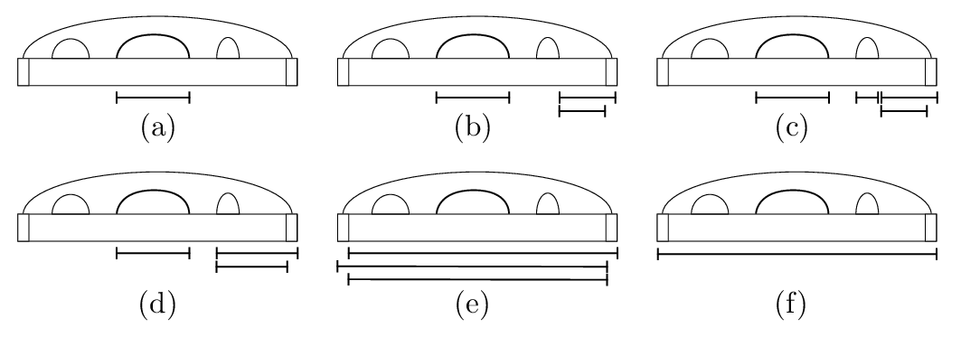
The computation in case 2 is illustrated in Fig. 6. Note that when in the loop in line 4, line 4(c) computes and . In both cases above the algorithm computes several local sequences of the form and , for some . These sequences are computed in order of decreasing values of and each sequence only depends on the previous one and recursively computed sequences. Hence, we only need to store a constant number of local sequences during the computation at .
4.4 Analysis
We first consider the time complexity of the algorithm. To do so we bound the total number of primitive operations. For each arc in there is initialize and meld operation and for each internal arc there is combine operation. Hence, the total number of initialize, meld, and combine operations is . To count the number of extend operations we first define for any arc the set as the set of positions inside but not inside any child arc of , that is,
For example, for in Fig. 1(a) is . The sets for all arcs is a partition of the positions in and thus . At an arc the algorithm performs extend operations and hence the total number of extend operations is . By Lemma 3 each primitive operation takes time and therefore the total running time of the algorithm is .
For the space complexity we bound the number of sequences stored by the algorithm. When the algorithm visits an arc we are currently processing a nested sequence of recursive calls corresponding to a path in from the root to . The number of sequences stored at each of these recursive calls is the total number of sequences stored. Consider an edge in from a parent to a child . If is heavy the recursive call to is done in line 1 of case 2 in the algorithm immediately at the start of the visit to . Therefore, no sequence at is stored. If is light the recursive call to is done in line 4(a). The algorithm stores at most sequences, namely , , and , where is the heavy child of . By Lemma 2 there are at most light ancestors of in and therefore the total space for stored sequences is . The additional space used by the algorithm is . Hence, we have the following result.
Lemma 4
Given nested arc-annotated strings and of lengths and , respectively, we can solve the nested arc-preserving subsequence problem in time and space .
5 Squeezing into Linear Space
We now show how to compress sequences into a compact representation using bits. Plugging the new representation into our algorithm the total space becomes as desired for Theorem 1.
Our compression scheme for sequences relies on the following key property of the values of .
Lemma 5
For any integers , , ,
Proof. Adding another base in front of the substring cannot increase the endpoint of an embedding of in and therefore . Furthermore, for any substring we can embed at most bases and at least bases in implying the remaining inequalities.
Let be indices in such that and consider the sequence
By Lemma 5 we have that is a non-increasing and non-negative sequence where is either or . We encode the sequence efficiently using two bit strings and defined as follows. The string is formed by the concatenation of bit strings , that is, , where denotes concatenation. The string is the single bit and , , is given by
Let denote the sum of bits in string . We have that and inductively . The string is the bit string of length consisting of a in each position where a substring in ends. Given and we can therefore uniquely recover . Since can decrease by at most the total number of s in is at most . The total number of s is at most and therefore . Hence, our representation uses bits. We can compress into and in a single scan in time. Reversing the process we can also decompress in time. Hence, we have the following result.
Lemma 6
We represent any sequence using bits. Compression and decompression takes time.
We modify our algorithm from Section 4 to take advantage of Lemma 6. Let be an internal arc in . Immediately before a recursive call to a light child of we compress the at most 3 sequences maintained at , namely , where is the heavy child, , and . Immediately after returning from the recursive call we decompress the sequences again.
The total number of compressions and decompressions is . Hence, by Lemma 6 the additional time used is and therefore the total running time of the algorithm remains . The space for storing the sequences becomes bits. Hence, the total space is . In conclusion, we have shown Theorem 1.
5.1 Avoiding Decompression
The above algorithm requires decompressions. We briefly describe how one can avoid these decompressions by augmenting the representation of sequences slightly. A rank/select index for a bit string supports the operations that returns the number of s in and that returns the position of the th in . We can construct a rank/select index in time that uses bits and supports both operations in constant time [20]. We add a rank/select index to the bit strings and in our compressed representation. Since these use bits this does not affect the space complexity. Let be a sequence compressed into bit strings and augmented with a rank/select index. For any , we can compute the element in constant time as
To see the correctness, first note that is end position of the th substring in . Therefore, is the sum of the bits in the first substrings of . This is and since the computation returns . In summary, we have the following result.
Lemma 7
We can represent any sequence in bits while allowing constant time access to any element.
The algorithm now only needs to compress sequences once. Whenever, we need an element of a compressed sequence we extract it in constant time as above. Hence, the asymptotic complexity of the algorithm remains the same.
References
- [1] J. Alber, J. Gramm, J. Guo, and R. Niedermeier. Computing the similarity of two sequences with nested arc annotations. Theor. Comput. Sci., 312(2-3):337–358, 2004.
- [2] R. Backofen, S. H. H. Bernhart, C. Flamm, C. Fried, G. Fritzsch, J. Hackermüller, J. Hertel, I. L. L. Hofacker, K. Missal, A. Mosig, S. J. J. Prohaska, D. Rose, P. F. F. Stadler, A. Tanzer, S. Washietl, and S. Will. RNAs everywhere: genome-wide annotation of structured rnas. J. Exp. Zoolog. B Mol. Dev. Evol., pages 1–25, 2007.
- [3] R. Backofen, G. M. Landau, M. Möhl, D. Tsur, and O. Weimann. Fast RNA structure alignment for crossing input structures. In Proc. 20th CPM, 2009.
- [4] V. Bafna, S. Muthukrishnan, and R. Ravi. Computing similarity between RNA strings. In Proc. 6th CPM, LNCS, volume 937, pages 1–16, 1995.
- [5] P. Bille and I. L. Gørtz. The tree inclusion problem: In optimal space and faster. In Proc. 32nd ICALP, LNCS, volume 3580, pages 66–77, 2005.
- [6] G. Blin, G. Fertin, R. Rizzi, and S. Vialette. What makes the Arc-Preserving Subsequence Problem hard? Trans. Comput. Sys. Bio. II, pages 1–36, 2005. Announced at ICCS 2005.
- [7] G. Blin and H. Touzet. How to compare arc-annotated sequences: The alignment hierarchy. In Proc. 13th SPIRE, LNCS, pages 291–303, 2006.
- [8] H.-J. Böckenhauer and D. Bongartz. Algorithmic Aspects of Bioinformatics (Natural Computing Series). Springer-Verlag New York, Inc., Secaucus, NJ, USA, 2007.
- [9] W. Chen. More efficient algorithm for ordered tree inclusion. J. Algorithms, 26:370–385, 1998.
- [10] P. Damaschke. A remark on the subsequence problem for arc-annotated sequences with pairwise nested arcs. Inf. Process. Lett., 100(2):64–68, 2006.
- [11] P. Evans. Algorithms and Complexity for Annotated Sequence Analysis. PhD thesis, University of Victoria, 1999.
- [12] A. Farris, G. Koelsch, G. Pruijn, W. van Venrooij, and J. Harley. Conserved features of Y RNAs revealed by automated phylogenetic secondary structure analysis. Nucl. Acids Res., 27(4):1070–1078, 1999.
- [13] J. Gramm, J. Guo, and R. Niedermeier. Pattern matching for arc-annotated sequences. ACM Trans. Algorithms, 2(1):44–65, 2006. Announced at FSTTCS 2002.
- [14] D. Harel and R. E. Tarjan. Fast algorithms for finding nearest common ancestors. SIAM J. Comput., 13(2):338–355, 1984.
- [15] K. Hellendoorn, P. Michiels, R. Buitenhuis, and C. Pleij. Protonatable hairpins are conserved in the 5’-untranslated region of tymovirus RNAs. Nucl. Acids Res., 24(24):4910–4917, 1996.
- [16] V. Juan, C. Crain, and C. Wilson. Evidence for evolutionarily conserved secondary structure in the H19 tumor suppressor RNA. Nucl. Acids Res., 28(5):1221–1227, 2000.
- [17] T. Kida. Faster pattern matching algorithm for arc-annotated sequences. In Federation over the Web, LNCS, volume 3847, pages 25–39, 2006.
- [18] P. Kilpeläinen and H. Mannila. Ordered and unordered tree inclusion. SIAM J. Comput., 24:340–356, 1995.
- [19] G. Lin, Z.-Z. Chen, T. Jiang, and J. Wen. The longest common subsequence problem for sequences with nested arc annotations. J. Comput. Syst. Sci., 65(3):465–480, 2002.
- [20] I. Munro. Tables. In Proc. 16th FSTTCS, LNCS, volume 1180, pages 37–42, 1996.
- [21] S. W. M. Teunissen, M. J. M. Kruithof, A. D. Farris, J. B. Harley, W. J. v. Venrooij, and G. J. M. Pruijn. Conserved features of Y RNAs: a comparison of experimentally derived secondary structures. Nucl. Acids Res., 28(2):610–619, 2000.
- [22] S. Vialette. On the computational complexity of 2-interval pattern matching problems. Theor. Comput. Sci., 312(2-3):223–249, 2004. Announced at CPM 2002.