A Ghost Story II: Ghosts, Gluons and the Gluon condensate beyond the IR of QCD
Abstract:
Beyond the deep IR, the analysis of ghost and gluon propagators still keeps very interesting non-perturbative information. The Taylor-scheme coupling can be computed and applied to obtain the parameter from Landau gauge lattice simulations. Furthermore, a dimension-two gluon condensate, that can be understood in the instanton liquid model, plays an important role in the game.
September 7-11 , 2009
ECT Trento, Italy
1 Introduction
Much work has been devoted in the last years to the study of the QCD running coupling constant determined from lattice simulations, as well in its perturbative regime [1, 2, 3, 4, 5, 6, 7, 8, 9] as in the deep infrared domain [10]. Only very recently [9, 11], the Green’s function approach to study the running coupling and then to estimate has been pursued by exploiting a non-perturbative definition of the coupling derived from the ghost-gluon vertex. The very infrared domain for the running of the coupling so defined has been discussed in the Olivier Pene’s talk. We aim to deal here with the running behaviour of this ghost-gluon coupling beyond the IR domain, above roughly 2-3 Gev.
We will show that the analysis of quenched lattice simulations leads to a non-perturbative determination of the running coupling in terms of two-point ghost and gluon Green functions and to obtain in pure Yang-Mills (). Furthermore, a very realistic estimate of , directly comparable with experimental determinations, will become an immediate possibility thanks to the many unquenched configurations which are presently available.
A precise determination of the non-perturbative coupling from the lattice also reveals a dimension-two non-zero gluon condensate in the landau gauge [10]. One needs then to describe the running with a formula including non-perturbative power corrections to be confronted with lattice estimates of the coupling. This procedure constitutes an optimal method for the identification of and of the gluon condensate [11]. Much work has been also done to investigate its phenomenological implications in the gauge-invariant world [12]. In particular, we will discuss the interpretation of this condensate in terms of the Yang-Mills semiclassical field background by applying the Instanton liquid model.
2 The ghost-gluon coupling
There is a large number of possibilities to define the QCD renormalized coupling constant, depending on the observable used to measure it and on the renormalization scheme. Actually, any observable which behaves, from the perturbative point of view, as provides a suitable definition for it. Among such quantities stand the 3-gluon and the ghost-gluon vertices, which have been widely used by the lattice community to get a direct knowledge of from simulations. Of course an important criterion to choose among those definitions will be how easy it is to connect it to other commonly used definitions, specially the one, and to extract from it fundamental parameters like .
A convenient class of renormalization schemes to work with on the lattice is made of the so-called schemes which are defined through the requirement that a given scalar coefficient function of the Green’s function under consideration take its tree-level value in a specific kinematical situation given up to an overall “renormalization scale”. To make the point clearer we recall 2 schemes which we have used in previous works on :
- •
The symmetric 3-gluon scheme in which one uses the 3-gluon vertex with
- •
The asymmetric 3-gluon scheme () in which the 3-gluon vertex is used with
In the present note we shall apply a specific -type renormalization scheme defined by fixing the (ghost and gluon) propagators and the ghost-gluon vertex at the renormalization point. Let us start by writing the ghost and gluon propagators in Landau gauge as follows,
| (1) |
being some regularisation parameter ( if, for instance, we specialise to lattice regularisation). The renormalized dressing functions, and are defined through :
| (2) |
with renormalization condition
| (3) |
Now, we will consider the ghost-gluon vertex which could be non-perturbatively obtained through a three-point Green function, defined by two ghost and one gluon fields, with amputated legs after dividing by two ghost and one gluon propagators. This vertex can be written quite generally as:
| (4) |
where is the outgoing ghost momentum and the incoming one, and renormalized according to:
| (5) |
The vertex involves two independent scalar functions. In the MOM renormalization procedure is fully determined by demanding that one specific combination of those two form factors (chosen at one’s will) be equal to its tree-level value for a specific kinematical configuration. We choose to apply MOM prescription for the scalar function that multiplies in eq. (4) and the renormalization condition reads11 1 In the case of zero-momentum gluon, an appropriate choice would be . This would make the renormalized vertex equal to its tree-level value at the renormalization scale.
| (6) |
where we prescribe a kinematics for the subtraction point such that the outgoing ghost momentum is evaluated at the renormalization scale, while the incoming one, , depends on the choice of several possible configurations; for instance: (symmetric configuration) or (asymmetric-ghost configuration).
On the other hand, the fields involved in the non-perturbative definition of the vertex in eq. (4) can be directly renormalized by their renormalization constants, and , and the same MOM prescription applied to the scalar combination also implies:
| (7) | |||||
We combine both eq. (6) and the first-line equation of (7) to replace and obtain the second line that shows the well-known relationship , where .
We turn now to the specific -type renormalization scheme defined by a zero incoming ghost momentum. Since those kinematics are the ones (and the only ones) in which Taylor’s well known non-renormalization theorem (cf. ref [13]) is valid we shall refer to this scheme as to the -scheme and the corresponding quantities will bear a subscript. Then, in eq (4), we set to and get
| (8) |
Now, Taylor’s theorem states that is equal to 1 in full QCD for any value of . Therefore, the renormalization condition eq. (6) implies and then
| (9) |
where we also apply the renormalization condition for the propagators, eqs. (2,3), to replace the renormalization constants, and , by the bare dressing functions. The remarkable feature of eq. (9) is that it involves only and so that no measure of the ghost-gluon vertex is needed for the determination of the coupling constant.
Equation (9) has extensively been advocated and studied on the lattice (see for instance reference [14]). However it must be stressed that the -scheme is the only one in which . Nevertheless the form (9) is used quite often in this case (for a kinematical configuration other than T-scheme’s) also as an approximation, specially in relation with the study of Dyson-Schwinger equations. An important remark is also in order here: in the very infrared domain, for phenomenological purposes (see for instance [15]), the coupling can be more properly defined by pulling a massive gluon propagator out from the ghost-gluon Green function used to build it [16].
2.1 Pure perturbation theory
A standard four-loop formula describing the running for the -scheme coupling,
| (10) | |||||
| with |
is obtained by inverting the -function of ,
| (11) |
where, as explained in [11], the coefficients can be computed in terms of , those for the -function of the coupling renormalizad according -scheme, , and of the anomalous dimensions for gluon and ghost propagators,
| (12) | |||||
Both anomalous dimensions need to be renormalized along MOM prescriptions (i.e., ) but expanded in terms of . The coefficients so obtained (the details and results of the computation can be found in [11]) appear to agree with those directly obtained in ref. [17] by the three-loop perturbative substracion of the ghost-gluon-gluon vertex in the QCD Lagrangian with the appropriate kinematical configuration (-scheme).
2.2 OPE power corrections
In order to extend the description of the running coupling down to energies as low as possible (of the order of 3 GeV) and to take full advantage of the lattice data we want to compare with, in order to reduce the systematic uncertainties, it is mandatory to take into account the gauge-dependent dimension-two OPE power corrections (cf. [7, 8, 10, 18]) to .
The leading power contribution to the ghost propagator,
| (13) |
can be computed using the operator product expansion [19] (OPE), as is done in ref. [20],
| (14) |
here is a local operator, regular when , and the Wilson coefficient contains the short-distance singularity. Eq. (14) involves a full hierarchy of terms, ordered according to their mass-dimension, among which only and contribute to eq. (13) in Landau gauge 22 2 The operators with an odd number of fields (; and ) cannot satisfy colour and Lorentz invariance and do not contribute a non-zero non-perturbative expectation value, and does not contribute either because of the particular tensorial structure of the ghost-gluon vertex. up to the order . Then, using eq. (14) into eq. (13), we obtain:
| (15) | |||||
where
| (16) | |||||
and the SVZ factorisation [21] is invoked to compute the Wilson coefficients. Thus, one should compute the “sunset” diagram of the last line of eq. (16), that binds the ghost propagator to the gluon condensate (where the blue bubble means contracting the color and lorentz indices of the incoming legs with ) to obtain the leading non-perturbative contribution (of course, the first Wilson coefficient gives trivially the perturbative propagator).
Finally, after the renormalization of the -condensate at the subtraction point , according to the MOM scheme definition, the ghost dressing function is written as:
| (17) |
where the multiplicative correction to the purely perturbative is determined up to corrections of the order or . As far as we do not deal with the anomalous dimension of the operator, factorising this purely perturbative ghost dressing function in eq. (17) is a matter of choice. However, the Wilson coefficient is also computed at the leading logarithm in ref. [11] and eq. (17) appears then to be a very good approximation up to this order.
We can handle in the same way (see refs.[7, 8]) the OPE power correction to the gluon propagator,
| (18) |
and obtain
| (19) | |||||
Then, after renormalization and appropriate projection, one gets for the gluon dressing function:
| (20) |
Finally, putting together the defining relation eq. (9) and the results eqs. (17,20) we get
| (21) | |||||
where is some perturbative scale and the running of the perturbative part of the evolution, , is of course described by the eq. (10) in the previous section. Again, the Wilson coefficient at leading logarithm for the T-scheme MOM running coupling is obtained in [11] and found not to induce a significant effect, provided that the coupling multiplying inside the bracket is taken to be renormalized also in T-scheme. Thus, eq. (21) describes pretty well the running of roughly above 3 Gev.
3 Data Analysis by the “plateau” method
In the following, as done in [11], we will apply a “plateau”-procedure exploiting eq. (21) to get a reliable estimate of the -parameter from lattice data. The goal being to get a trustworthy estimate of the -parameter, one could attempt to do it by inverting the perturbative formula eq. (10) and using in the inverted formula the lattice estimates of the running coupling obtained by means of eq. (9) for as many lattice momenta as possible. Then, one should look for a “plateau” of in terms of momenta in the high-energy perturbative regime (this was done with the coupling defined by the three-gluon vertex in [4, 5]). In the next subsection, fig. 1.(a) shows the estimates of so calculated for the lattice data presented in ref. [20, 22] over GeV2.
However, in order to take advantage of the largest possible momenta window one can use instead eq. (21). In this way we shall hopefully be able to extend towards low momenta the region over which to look for the best possible values of the gluon condensate and of 33 3 This increases the statistics and reduces errors. It also avoids some possible systematic deviation appearing when lattice momentum components, in lattice units, approach (Brillouin’s region border).. In other words, one requires the best-fit to a constant of
| (22) |
where is obtained by inverting the perturbative four-loop formula, eq. (10), and results from the best-fit (it appeared written in terms of the gluon condensate in eq. (21) ). Thus, reaches a “plateau” (if it does) behaving in terms of the momentum as a constant that we will take as our estimate of . Of course, this is nothing but a fitting strategy for a 2-parameters ( and ) fit of the estimates of eq. (9) from lattice data.
3.1 Results for pure Yang-Mills ()
The quenched lattice data that we will exploit now were presented for the first time in ref. [22]. We refer to this work for all the details concerning the lattice implementation: algorithms, action, Faddeev-Popov operator inversion, etc. The parameters of the whole set of simulations are described in table 1
| Volume | (GeV) | Number of confs. | |
|---|---|---|---|
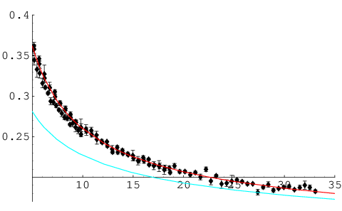
In fig. 1.(a), we show the estimates of obtained when interpreting the lattice coupling computed by eq. (9) for any momentum GeV2 in terms of the inverted four-loop perturbative formula for the coupling, eq. (10). The estimates systematically decrease as the squared momentum increases until around 22 GeV2; above this value, only a noisy pattern results. In fig. 1.(b), the same is plotted but inverting instead the non-perturbative formula including power corrections, eq. (21). The value of the gluon condensate has been determined by requiring a “plateau” to exist (as explained in the previous section) over the total momenta window.
|
|


One should realize that the non-perturbative analysis seems to indicate that the perturbative regime is far from being achieved at GeV. This is also illustrated by figure 2.a in which, adopting for the value MeV which results from the non-perturbative analysis, we plot against the square of the renormalization momentum the coupling constant as computed by means of the non-perturbative formula (21) (red curve) and of the perturbative one (10) (blue curve). Displayed are also the lattice data, i.e. the values of obtained from eq. (9).
 |
 |
| (a) | (b) |
Thus, one can conclude that our best-fit parameters incorporating only 44 4 The error analysis is deeply discussed in [11]. statistical errors are:
| (23) |
These values are in very good agreement with the previous estimates from quenched lattice simulations of the three-gluon Green function [7, 8] or, in the case of , from the implementation of the Schrödinger functional method [2], although slightly larger than the one obtained by the ratio of ghost and gluon dressing functions [20] (see fig. 2.(b) and tab. 2).
4 About the nature and the size of the gluon condensate
The nature of the dimension-two gluon condensate, as well as its possible phenomenological implications, have been discussed in many works in the last few years (see for instance [12, 18]). In particular, we presented some indications supporting the idea that the low-momentum gluon correlation functions could be nicely described in terms of the semiclassical instanton background for the gauge field [23], and used an instanton liquid picture to estimate the size for this gluon condensate in Yang-Mills [10]. Indeed, the gauge field in the instanton picture and within the sum-ansatz approach, can be written in the singular Landau gauge as
| (24) |
where is the bare gauge coupling in terms of the lattice parameter , is known as ’t Hooft symbol and represents the color rotations embedding the canonical SU(2) instanton solution in the SU(3) gauge group, () being an SU(2) (SU(3)) color index. The sum is extended over all the instantons and anti-instantons (we should then replace the ’t Hooft symbol by ) in the classical background of the gauge configuration. is the instanton profile function. If we consider the profile of the BPST solution for an isolated instanton, we get
| (25) |
where () stands for the total number of instantons (anti-instantons). On the other hand, if we neglect instanton position and color correlations, eq. (24) leads for the -gluon Green function to
| (26) |
for ; being the instanton density. It depends on the functional of the general instanton profile, , and means the average over instanton sizes with a given normalised instanton radius distribution, . Then, two interesting limits appear where some results not depending on the instanton profile can be obtained:
- •
- •
For , as asymptotically behaves as in the large limit, one obtains
(28)
Thus, eq. (28) provides us with large-momentum limits for the two and three-gluon Green functions behaviour which do not depend on the radius distribution nor on the instanton profile. However, the large-momentum lattice correlation function being dominated by the short-distance quantum fluctuations, whether such a behaviour occurs can be only detected after performing some “cooling” procedure [25] to kill the higher energy modes. This is done in [23] and, as can be seen in fig. 3.a, the expected () power behaviour clearly emerges for the two-gluon (three-gluon) Green function after “cooling”. This is a good indication for the success of the instanton picture in describing the gluon correlation functions. However, as the “cooling” has been proved to alter the configuration (instanton sizes become distorted, instanton and anti-instanton anhiliate to each other…), the power-law given by eq. (27), which is thought to be followed by the “uncooled” gluon correlators in the low-momentum regime, offers a more reliable “instanton detector”. In ref. [24], eq. (27) is shown to work for a three-gluon coupling computed from several lattice simulations (see fig. 3.b taken from [24]) and the instanton density is estimated to be fm-4.
 |
 |
 |
| (a) | (b) |
Then, this estimate of the instanton density and the average instanton radius, fm (measured, for instance, in [23] and being close to the phenomenological prediction, fm), can be applied to eq. (25) to give: . There is of course no exact recipe to compare this estimate with the OPE one, since the separation between the semiclassical non perturbative domain and the perturbative one cannot be exact 55 5 One may appeal to the fact that at the renormalisation point , the radiative corrections are minimised; therefore a semiclassical estimate must best correspond to at some reasonable , which one could guess to be a typical scale of the problem as or some gluon mass.. However, both lie prettily on the same ballpark.
5 Conclusion
We have demonstrated that, in the particular -scheme, the coupling defined from the ghost-gluon vertex is obtained by only dealing with two-point Green functions. Some interesting non-perturbative information can be furthermore distilled from the running analysis of this coupling beyond the deep IR: the parameter (usually expressed in the -scheme), computed here for pure Yang-Mills from Landau gauge lattice simulations, and a gauge-dependent dimension-two gluon condensate. The latter is interpreted and sized by invoking an instanton liquid picture, which successfully describes the low-momentum gluon correlations.
References
- [1] G. S. Bali and K. Schilling, Phys. Rev. D 47 (1993) 661 [arXiv:hep-lat/9208028].
- [2] M. Luscher, R. Sommer, P. Weisz and U. Wolff, Nucl. Phys. B 413 (1994) 481; S. Capitani, M. Luscher, R. Sommer and H. Wittig [ALPHA Collaboration], Nucl. Phys. B 544 (1999) 669
- [3] G. M. de Divitiis, R. Frezzotti, M. Guagnelli and R. Petronzio, Nucl. Phys. B 433 (1995) 390
- [4] B. Alles et al. Nucl. Phys. B 502 (1997) 325 [arXiv:hep-lat/9605033].
- [5] P. Boucaud, J. P. Leroy, J. Micheli, O. Pene and C. Roiesnel, JHEP 9810 (1998) 017
- [6] P. Boucaud et al., JHEP 0004 (2000) 006 [arXiv:hep-ph/0003020].
- [7] Ph. Boucaud, A. Le Yaouanc, J.P. Leroy, J. Micheli, O. Pène, J. Rodriguez-Quintero, Phys. Lett. B493(2000) 315.
- [8] Ph. Boucaud,A. Le Yaouanc, J.P. Leroy, J. Micheli, O. Pène, J. Rodriguez-Quintero, Phys. Rev. D 63(2001) 114003; F. De Soto and J. Rodriguez-Quintero, Phys. Rev. D 64 (2001) 114003 .
- [9] A. Sternbeck, K. Maltman, L. von Smekal, A. G. Williams, E. M. Ilgenfritz and M. Muller-Preussker, PoS LAT2007 (2007) 256 [arXiv:0710.2965 [hep-lat]].
- [10] P. Boucaud et al., Phys. Rev. D 66 (2002) 034504; JHEP 0304 (2003) 005; Phys. Rev. D 70 (2004) 114503.
- [11] Ph. Boucaud et al., Phys. Rev. D 79 (2009) 014508 [arXiv:0811.2059 [hep-ph]].
- [12] F. V. Gubarev and V. I. Zakharov, Phys. Lett. B 501 (2001) 28 [arXiv:hep-ph/0010096].
- [13] J. C. Taylor, Nuclear Physics B33 (1971) 436
- [14] L. von Smekal, R. Alkofer and A. Hauck, Phys. Rev. Lett. 79 (1997) 3591 [arXiv:hep-ph/9705242].
- [15] D. Binosi and J. Papavassiliou, Phys. Rept. 479 (2009) 1 [arXiv:0909.2536 [hep-ph]].
- [16] A. C. Aguilar, D. Binosi, J. Papavassiliou and J. Rodriguez-Quintero, Phys. Rev. D 80 (2009) 085018
- [17] K. G. Chetyrkin and A. Retey, [arXiv:hep-ph/0007088]; T. van Ritbergen, J. A. M. Vermaseren and S. A. Larin, Phys. Lett. B 400 (1997) 379.
- [18] D. Dudal, H. Verschelde and S. P. Sorella, Phys. Lett. B 555 (2003) 126 ; K. I. Kondo, Phys. Lett. B 572 (2003) 210 ; [arXiv:hep-th/0306195].
- [19] R. Wilson, Phys. Rev. 179 (1969) 1499.
- [20] Ph. Boucaud et al., JHEP 0601 (2006) 037 [arXiv:hep-lat/0507005]; Phys. Rev. D 63(2001) 114003.
- [21] M.A. Shifman, A.I. Vainshtein, V.I. Zakharov, Nucl. Phys. B 147(1979) 385; M.A. Shifman, A.I. Vainshtein, M.B. Voloshin, V.I. Zakharov, Phys. Lett. B 77(1978) 80.
- [22] Ph. Boucaud et al., Phys. Rev. D 72 (2005) 114503 [arXiv:hep-lat/0506031].
- [23] Ph. Boucaud et al. JHEP 0503 (2005) 046 ; Phys. Rev. D 70 (2004) 114503.
- [24] P. Boucaud et al., JHEP 0304 (2003) 005 [arXiv:hep-ph/0212192].
- [25] M. Teper, Phys. Lett. B 162 (1985) 357.