de Sitter Thick Brane Solution in Weyl Geometry

The possibility that our world is trapped in a four-dimensional submanifold (called brane) embedded in a fundamental multi-dimensional space-time (called bulk) has been increasing interest during recent years (see [1, 2] for summary of introduction, and reference therein). The strong motivations originate from the string/M theory. With the help of the brane scenario, one could possibly solve some disturbing problem of high-energy physics, such as the hierarchy problems (the problem of why the electroweak scale $M_{EW}\sim 1$ TeV is so different from the Planck scale $M_{pl}\sim 10^{16}$ TeV ) and the cosmological constant problem [3, 4, 5, 6, 7, 8]. In this scenario, Standard Model matter fields are confined to a 3-brane, while the gravity could propagate in the whole bulk. The most well-known models within are Arkani-Hamed-Dimopoulos-Dvali (ADD) [3, 4] and Randall-Sundrum (RS) [5, 6] models put forward in the end of 90’s. They can achieve a Newtonian gravitation law in macroscopic scale, which is compatible with the observational fact. What preeminence in RS model is that it suggests a possibility that the extra dimensions may not be compact any more, namely the size of extra dimensions can be even infinite.

However, both the models above are assumed that the brane is infinitely thin. Although with the idealized models many interesting results have been obtained, from a more realistic point of view, a brane should have the thickness. For this reason, the emphasis of study has shifted toward the thick brane scenario [9, 10, 11, 12, 13, 14, 15, 16, 17, 18, 19, 20, 21, 22, 23, 24, 25, 26, 27, 28, 29, 30, 31, 32, 33]. An interesting feature of thick brane scenario based on gravity coupled to scalar is that one can achieve a brane naturally without introducing a delta function by hand in the action to create a brane. And the scalar could further provide the “material” to make the thick brane. In many multidimensional field theories coupled to gravity there are solutions of topological defects. They have lead to a richer variety of thick brane worlds [16].

Most investigations of brane worlds are considered in Riemann geometry. In this paper, we are interested in the thick branes based on a Weyl-integrable geometry, which is a generalization of Riemann geometry.

As is shown in (1) [34], we can see there are two type generalizations of Riemann geometry, namely, the Riemann-Cartan and the Weyl geometry. In Riemann-Cartan geometry, the connection is asymmetric and the antisymmetric piece of the connection is represented as torsion $T$ introduced by Cartan. In contrast to Riemann-Cartan geometry, the connection is no longer metric compatible in Weyl geometry, i.e., it involves a geometric scalar $\omega$ in the definition of connection and the covariant derivative of metric tensor is non-vanishing. The field related to this violation of the metricity condition is called nonmetricity $Q$. So Weyl geometry allows for possible variations in the length of vectors during parallel transport. When $T=0$ the Riemann-Cartan geometry degenerates into Riemann, and when $Q=0$ the Weyl geometry also degenerates into Riemann geometry. More precisely, a Weyl geometry is an affine manifold specified by $(g_{MN},\omega)$, where $g_{MN}$ is the metric tensor and $\omega$ is the geometric scalar $\omega$. Since a conformal transformation can map a Weyl manifold into a Riemann one, the particular type of gauge geometries is called conformally Weyl or Riemann integrable space-time [35]. On the other hand, Weyl integrable manifold is invariant under a Weyl rescaling (see, (6) for detail), when this invariance is broken, the Weyl scalar function $\omega$ transforms into an observable field which generates the smooth thick brane configurations. Thus in Weyl geometry the fundamental role in the generation of thick brane configurations is ascribed to the geometric Weyl scalar field, which is not a bulk field now.

In Refs. [14, 35, 36, 37], the authors have studied brane world scenario in the frame of Weyl geometry, and achieved various solutions respected to Minkowski thick branes. For most of these branes [35, 36], there exist a single bound state which represents a stable 4-dimensional graviton and the continuum spectrum of massive modes of KK excitations without mass gap for a volcano potential. While in [14], the KK spectrum is quantized for an infinite square-like potential wall, and in [37], there exist one massless bound state, one massive KK bound state and the delocalized continuum spectrum for a modified P$\ddot{\text{o}}$schl-Teller potential. These give a claim that Weylian structures mimic, classically, quantum behavior does not constitute a generic feature of these geometric manifolds [36]. In Refs. [38, 39], the authors have considered the localization and mass spectrum problems of matter fields on these various Minkowski thick branes. An interesting study in [39] shows that for scalars there are two bound states (one is normalizable massless mode), for spin one vectors there is only one normalizable massless bound state, and for spin half fermions, the total number of bound states is determined by the coupling constant $\eta$: when $\eta=0$, there are no any localized fermion KK modes including zero modes for both left and right chiral fermions, and when $\eta>0$ ($\eta<0$), the number of bound states of right chiral fermions is one less (more) than that of left chiral fermions and in both cases ($\eta>0$ and $\eta<0$), only one of the zero modes for left chiral fermions and right chiral fermions is bound and normalizable.

We will consider a de Sitter thick brane based on gravity coupled to scalars on a Weyl integrable manifold in this paper, and try to find a solution of de Sitter thick brane from a pure geometrical Weyl action in five dimensions. The organization of the paper is as follows: In Sec. 2, we briefly review the Weyl geometry. In Sec. 3, we consider a de Sitter thick brane solution on the weyl manifold and find a solution of the model. In Sec. 4, we briefly consider the gravitational and scalar perturbations of the structure. In Sec. 5, we derive the effective Newtonian potential on the brane. And finally, the conclusion is given in Sec. 6.

A non-Riemann generalization of Kaluza-Klein theory is based on the following five-dimensional action [14]:

where $M_{5}^{W}$ is a five-dimensional Weyl-integrable manifold specified by the pair $(g_{MN},\omega)$, $g_{MN}$ is the metric $(M,N=0,1,2,3,5)$ and $\omega$ is a scalar function. In this manifold the Weylian Ricci tensor reads $R_{MN}=\Gamma_{MN,A}^{A}-\Gamma_{AM,N}^{A}+\Gamma_{MN}^{P}\Gamma_{PQ}^{Q}-\Gamma_{MQ}^{P}\Gamma_{NP}^{Q}$, where the affine connection of $M_{5}^{W}$ is $\Gamma_{MN}^{P}=\{_{MN}^{P}\}-\frac{1}{2}(\omega_{,M}\delta_{N}^{P}+\omega_{,N}\delta_{M}^{P}-g_{MN}\omega^{,P})$ with $\{_{MN}^{P}\}$ the Christoffel symbol. The parameter $\xi$ is a coupling constant, and $U(\omega)$ is a self-interaction potential for the scalar field. Since the scalar field $\omega$ enters in the definition of the affine connection of the Weyl manifold, the Weyl action is actually pure geometrical.

Weyl integrable manifold is invariant under the Weyl rescaling,

where $\Omega^{2}$ is a smooth function on $M_{5}^{W}$. In general, this invariance is broken by the self-interaction potential $U(\omega)$. But from the relation (6), we know that $U\rightarrow\Omega^{-2}U$ is the only transformation preserves such an invariance. Thus the potential will be $U(\omega)=\lambda e^{-\omega}$, where $\lambda$ is a coupling constant. When the Weyl invariance is broken, the scalar field could transform from a geometric object into an observable degree of freedom which generates the smooth thick brane configurations.

In order to find solutions of the above theory, we shall use the conformal technique to map the Weyl frame into the Riemann one. Under the conformal transformation $g_{MN}=e^{\omega}\hat{g}_{MN}$, the Weylian affine connection becomes the Christoffel symbol $\Gamma^{P}_{MN}\rightarrow\{_{MN}^{P}\}$, and the Weylian Ricci tensor becomes the Riemannian Ricci tensor. In consequence, via the conformal transformation, one recovers the Riemannian structure on the manifold $M_{5}^{R}$. Now the Weylian action (5) is mapped into a Riemann one:

where $\hat{U}(\omega)=e^{\omega}U(\omega)$ and all the hatted magnitudes and operators refer to the Riemann frame. Thus, one obtains a theory which describes five-dimensional gravity coupled to a scalar field with a self-interaction potential in the Riemann frame.

By considering the variation of the metric $\hat{g}^{MN}$ and the scalar function $\omega$, we have the set of field equations from (7):

In Refs. [14, 35, 36, 37], the authors studied thick brane solutions to the theory (5), and they considered the metric that respects four-dimensional Poincar$\acute{\text{e}}$ invariance:

i.e., the Minkowski thick brane solutions in Weyl Geometry, where $e^{2A(y)}$ is the warp factor and $y$ stands for the extra coordinate. The localization and mass spectrum problems of matter fields on the Minkowski thick branes were discussed in Refs. [38, 39].

The authors of [14] have considered the problem of $Z_{2}$-symmetric manifolds. They have chosen $\xi=-(1+k)/(4k)$ and left $k$ as an arbitrary parameter except for $k=-4/3$. The following solution was found:

The authors of [35] have considered another simplified case when $k=-4/3$ and left $\xi$ as an arbitrary parameter except for $\xi=-1/16$. Their solution is

Obviously, the first solution (10) is symmetric with respect to $y$ coordinate, and the second solution is also a symmetric one if we perform a translation of $y$ axis.

In this paper, we consider a de Sitter thick brane solution in a pure geometric five-dimensional Weyl space-time. The line element for the space-time with planar-parallel symmetry is assumed as

where $\beta$ is the de Sitter parameter and related to the 4-dimensional cosmological constant of the brane. Under the conformal transformation $g_{MN}=e^{\omega}\hat{g}_{MN}$, the de Sitter metric (12) is mapped into

where $2\sigma=2A-\omega$.

Now the expressions for Ricci tensor and the scalar curvature in the Riemann frame read

where the prime denotes derivative with respect to the fifth coordinate $y$. The five-dimensional stress-energy tensor is given by

thus, its four-dimensional and five-dimensional components are given through the following expressions:

For simplicity, using the pair of variables $X\equiv\omega^{\prime}$ and $Y\equiv 2A^{\prime}$, we obtain a set of equations from (8), (13) and (3):

Though we have got the field equations by performing a conformal transformation $\hat{g}_{AB}=e^{-\omega}g_{AB}$ to map the Weyl manifold structure into the Riemann one, the solutions corresponding to the Eqs. (21) are harder to get than the similar equations in Ref. [14] for the flat brane (just set $\beta=0$ in Eqs. (21)). So, in order to simplify the model, we make a coordinate transformation of the form $dy=e^{A(z)}dz$. Then the metric (13) will be rewrote as:

Now repeating our calculation above, the expressions for the Ricci tensor and the scalar curvature corresponding to the metric (22) in the Riemann frame read:

The stress-energy tensor is given through the following expressions:

So the set of field equations with the new conformally metric (22) now read

where the prime denotes derivative with respect to $z$. If we choose the parameter $\xi=1/3$, and define $\hat{V}(\omega)=3\hat{U}(\omega)$, we can rewrite Eq. (29) as follows:

This set of equations is identical with the field equations of the de Sitter thick brane in the Riemann geometry [13, 40, 41, 42, 43, 44, 45, 46]. Here, we can achieve a $Z_{2}$-symmetric solution refer to $z$ coordinate when we consider a symmetric domain wall de Sitter expansion in five dimensions for a sine-Gordon potential [47, 48]

with $p=15\beta^{2}$, $q=1/\sqrt{3}$, $v=-15\beta^{2}/2$ and $\beta>0$. The warp factor of the metric (22) on Riemann manifold and the scalar $\omega$ are

From $\hat{U}(\omega)=e^{\omega}U(\omega)$ and Eq. (31), we have the potential in the original action (5) on the Weyl manifold:

From the relation $e^{2\sigma}=e^{2(A-\omega)}$, the warp factor $e^{2A(z)}$ is given by

The shapes of the scalar $\omega$, the potentials $\hat{U}(\omega)$ in the Riemannian structure and $U(\omega)$ in the Weylian one, the warp factors $e^{2\sigma}$ on the Riemann manifold and $e^{2A}$ on the Weyl manifold are shown in Figs. 1, 2 and 3, respectively. We can see that the scalar field takes values $\pm\sqrt{3}\pi/4$ at $z\rightarrow\pm\infty$, corresponding to the two minima of the potential with cosmological constant $\Lambda=0$. So the scalar is actually a kink solution, which provides a thick brane realization of the brane world as a domain wall in the bulk. In the Riemannian structure, the potential $\hat{U}(\omega)$ and the warp factor are symmetric, but in the Weylian one, they are asymmetric.

Now from $dy=e^{A(z)}dz$, we can calculate the relation between the original space-time coordinate $y$ in metric (13) and $z$ in (22). However, we could only achieve a numerical function curve $y=y(z)$ in Fig. 4 (left). The scalar field in $y$ coordinate is plotted in Fig. 4 (right).

We can find that the scalar $\omega(y)$ is asymmetric but still a kink-like solution in $y$ coordinate. We display the shapes of the warp factors $e^{2\sigma(y)}$ and $e^{2A(y)}$ in Fig. 5. The figure shows that the warp factor $e^{2\sigma(y)}$ is no longer symmetric even in the Riemannian structure, though the maximum is still at the origin of the $y$ coordinate. So it will not preserve $Z_{2}$-symmetry in the Riemann manifold in the $y$ coordinate.

The energy density of the scalar matter on the Riemann manifold is given by the null-null component of the stress-energy tensor (28):

The shape of the energy density $\hat{\rho}$ is plotted in Fig. 6 in $z$ and $y$ coordinates, respectively. The figures clearly show that the energy density $\hat{\rho}$ distributes along extra coordinate, so it does not stand for a thin brane any more, and $1/\beta$ plays the role of the brane thickness. The energy density has a maximum at the origin of the coordinate, and vanishes asymptotically at $y=\pm\infty$, so the scalar matter mainly distributes on the brane. The energy density is symmetric in $z$ coordinate while asymmetric in $y$.

Firstly, we consider the gravitational perturbation in the metric (22):

Here $h_{\mu\nu}$ is the tensor perturbation of the metric, and it satisfies the transverse traceless condition [9, 13, 49],

where $\nabla$ denotes the covariant derivative with respect to the four-dimensional metric $q_{\mu\nu}$. The equation for $h_{\mu\nu}$ is given by [13, 49]

where $\Box\equiv q^{\mu\nu}\nabla_{\mu}\nabla_{\nu}$. Here we can define the four-dimensional mass of a KK excitation as

Furthermore, we can decompose $h_{\mu\nu}$ in the form

where $\varepsilon_{\mu\nu}$ satisfies the transverse traceless condition

Now considering (39) and (40), Eq. (38) can be rewritten as

So it turns into a Schr$\ddot{\text{o}}$dinger equation form, and the effective potential reads

The spectrum of the eigenvalue $m^{2}$ parameterizes the spectrum of the observed four-dimensional graviton masses. And obviously, there exists a zero mode which refers to $m=0$. From Eq. (42) with $m=0$, we can easily get

It can easily be seen that this zero mode is normalizable, and $c_{0}=\sqrt{\frac{2\beta\Gamma({5}/{4})}{\sqrt{\pi}\;\Gamma({3}/{4})}}$ is a normalization constant. So the 4D gravity can be produced by the zero mode [6, 9, 10, 11, 13].

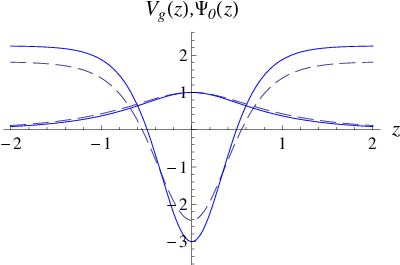
The shapes of the potential and the zero mode are plotted in Fig. 7. The figure shows that the gravitational zero mode localizes around $z=0$, and vanishes at each side asymptotically. The effective potential is actually a modified P$\ddot{\text{o}}$schl-Teller potential. From (43) we known that the potential barriers at each side approach to a maximum $V_{g}^{max}=9\beta^{2}/4$ when $z\rightarrow\pm\infty$, so there will be exist a set of continuous KK modes $\Psi_{m}(z)$, and there is a mass gap between the massless zero mode and the massive continuous KK modes. The existence of the gap is universal in various kinds of de Sitter 3-brane model [13, 49]. It can be shown that there is no any other bound KK mode beside the zero mode for the potential (43).

Next, we consider the scalar perturbation. Following the arguments in Refs. [13, 49], one can get the scalar perturbations in the metric (22) with the longitudinal gauge:

The equations of the scalar perturbation in the Schr$\ddot{\text{o}}$dinger-like form are read as [49]:

where $\Box\equiv q^{\mu\nu}\nabla_{\mu}\nabla_{\nu}$, $\delta\omega$ is the perturbation of background scalar $\omega$, and $V_{s}(z)$ is the effective potential of the scalar perturbation with the expression

Now we decompose $\Phi(x,z)$ according to (47) in the form

Then substitute it into Eq. (47), we get

where $m$ is the 4-dimensional effective mass of the scalar perturbational field. Now Eq. (50a) can be explicitly expressed as

i.e.,

So $X(x)$ can be decomposed as

Then we get

The solution of Eq. (54a) is simply achieved as $S_{k}(x^{i})=ce^{-i\delta_{ij}k^{i}x^{j}}$, where $c$ is a constant. Thus we will focus on Eq. (54b). The solution is

where $c_{1}$ and $c_{2}$ are integration constants, $\varsigma=\sqrt{\frac{9}{4}\beta^{2}-m^{2}}$, and J is the Bessel function. Now we expand $T_{km}(t)$ about the point $\frac{|\vec{k}|}{\beta}e^{-\beta t}\sim 0$ ($t\rightarrow\infty$):

where $c^{\prime}_{1}$ and $c^{\prime}_{2}$ are constants independent of time.

Case 1:  When $m^{2}>\frac{9}{4}\beta^{2}$, $\varsigma$ is imaginary. We define $\varsigma=i\zeta$ with $\zeta>0$. Now (56) can be rewritten as

Fig. 8a shows that, in this case, $T_{km}(t)$ vanishes at $t\rightarrow\infty$, i.e, the scalar perturbation disappears after a period of time. So we can see the structure is stable in this case.

Case 2:  When $0<m^{2}\leq\frac{9}{4}\beta^{2}$, $\varsigma$ is real and satisfy $0\leq\varsigma<\frac{3}{2}\beta$. Eq. (56) shows that $T_{km}(t)$ is actually suppressed by $t$, and vanishes at $t\rightarrow\infty$, just as shown in Fig. 8b. So the structure is also stable in this case.

Case 3:  When $m^{2}=0$, $\varsigma=\frac{3}{2}\beta$, the high order terms $\mathcal{O}\left(e^{-\left(\frac{5}{2}\beta-\varsigma\right)t}\right)$ and $\mathcal{O}\left(e^{-\left(\frac{5}{2}\beta+\varsigma\right)t}\right)$ in the expanding expression (56) are suppressed by $t$. While the first term in (56) is a constant $c^{\prime}_{1}=c_{1}$. If $c_{1}=0$, $T_{km}(t)$ also converges to zero when $t\rightarrow\pm\infty$, so the structure is stable. If $c_{1}\neq 0$, $T_{km}(t)$ will converge to the constant $c_{1}$ (see Fig. 9a), i.e., some slight scalar perturbations will always exist but not enormously affect the stability of the brane. So in this case we can say that the structure is also stable.

Case 4:  When $m^{2}<0$, $\varsigma$ is real and satisfy $\varsigma>\frac{3}{2}\beta$, the first term in (56) is divergent at $t\rightarrow\infty$ (see Fig. 9b). This means that in this case the scalar perturbation is divergent, and the structure is unstable under the scalar perturbation.

From above discussion, it is shown that the structure is stable when $m^{2}\geq 0$, while it is unstable when $m^{2}<0$.

We next focus on Eq. (50b), where $V_{s}(z)$ is the effective potential of the scalar perturbation. For (32a) and (32b), we have

From the expression of the above effective scalar perturbational potential, we can see that $V_{s}(z)$ approaches to $\frac{9}{4}\beta^{2}$ when $z\rightarrow\pm\infty$. Furthermore, $V_{s}(z)$ satisfies $V_{s}(z)>\frac{9}{4}\beta^{2}$ and is always convex and non-negative. Fig. 10 shows the potential with virous cases about the parameter $\beta$. From the Schr$\ddot{\text{o}}$dinger-like equation (50b), we can conclude that there are only KK modes with eigenvalues $m^{2}>\frac{9}{4}\beta^{2}$. This coincides with case 1. So the structure is stable under the scalar perturbations. The explicit argument about the stable problem of scalar perturbations could be seen in Ref. [49].

References

- [1] V.A. Rubakov, Large and infinite extra dimensions, Phys. Usp. 44 (2001) 871, arXiv:hep-ph/0104152.
- [2] C. Cski, TASI Lectures on Extra Dimensions and Branes, arXiv:hep-ph/0404096.
- [3] N. Arkani-Hamed, S. Dimopoulos and G. Dvali, The hierarchy problem and new dimensions at a millimeter, Phys. Lett. B 429 (1998) 263;
- [4] I. Antoniadis, N. Arkani-Hamed, S. Dimopoulos and G. Dvali, New dimensions at a millimeter to a Fermi and superstrings at a TeV, Phys. Lett. B 436 (1998) 257.
- [5] L. Randall and R. Sundrum, A Large Mass Hierarchy from a Small Extra Dimension, Phys. Rev. Lett. 83 (1999) 3370;
- [6] L. Randall and R. Sundrum, An alternative to compactification, Phys. Rev. Lett. 83 (1999) 4690.
- [7] C. Cski, M. Graesser, C. Kolda and J. Terning, Cosmology of One Extra Dimension with Localized Gravity, Phys. Lett. B 462 (1999) 34, arXiv:hep-ph/9906513;
- [8] J.M. Cline, C. Grojean and G. Servant, Cosmological Expansion in the Presence of an Extra Dimension, Phys. Rev. Lett. 83 (1999) 4245, arXiv:hep-ph/9906523.
- [9] O. DeWolfe, D.Z. Freedman, S.S. Gubser and A. Karch, Modeling the fifth dimension with scalars and gravity, Phys. Rev. D 62 (2000) 046008.
- [10] M. Gremm, Four-dimensional gravity on a thick domain wall, Phys. Lett. B 478 (2000) 434.
- [11] C. Cski, J. Erlich, T. Hollowood and Y. Shirman, Universal Aspects of gravity localized on thick branes, Nucl. Phys. B 581 (2000) 309.
- [12] A. Campos, Critical phenomena of thick brane in warped space-time, Phys. Rev. Lett. 88 (2002) 141602.
- [13] A.Z. Wang, Thick de Sitter brane worlds, dynamic black holes and localization of gravity, Phys. Rev. D 66 (2002) 024024, arXiv:hep-th/0201051.
- [14] O. Arias, R. Cardenas and I. Quiros, Thick Brane Worlds Arising From Pure Geometry, Nucl. Phys. B 643 (2002) 187, arXiv:hep-th/0202130.
- [15] V. Dzhunushaliev, V. Folomeev and M. Minamitsuji, Thick de Sitter brane solutions in higher dimensions, Phys. Rev. D 79 (2009) 024001, arXiv:0809.4076[gr-qc].
- [16] V. Dzhunushaliev, V. Folomeev and M. Minamitsuji, Thick brane solutions, Rept. Prog. Phys. 73 (2010) 066901, arXiv:0904.1775[gr-qc].
- [17] A. Herrera-Aguilar, D. Malag¨®n-Morej¨®n, R.R. Mora-Luna, U. Nucamendi, Aspects of thick brane worlds: 4D gravity localization, smoothness, and mass gap, Mod. Phys. Lett. A 25 (2010) 2089, arXiv:0910.0363[hep-th].
- [18] C.A.S. Almeida, M.M. Ferreira Jr., A.R. Gomes, R. Casana, Fermion localization and resonances on two-field thick branes, Phys. Rev. D 79 (2009) 125022, arXiv:0901.3543[hep-th].
- [19] Y.-X. Liu, L. Zhao and Y.-S. Duan, Localization of Fermions on a String-like Defect, JHEP 0704 (2007) 097;
- [20] L. Zhao, Y.-X. Liu and Y.-S. Duan, Fermions in gravity and gauge backgrounds on a brane world, Mod. Phys. Lett. A 23 (2008) 1129.
- [21] Y.-X. Liu, J. Yang, Z.-H. Zhao, C.-E Fu, Y.-S. Duan , Fermion Localization and Resonances on A de Sitter Thick Brane, Phys. Rev. D 80 (2009) 065019, arXiv:0904.1785[hep-th];
- [22] Y.-X. Liu, C.-E Fu, L. Zhao, Y.-S. Duan, Localization and Mass Spectra of Fermions on Symmetric and Asymmetric Thick Branes, Phys. Rev. D 80 (2009) 065020, arXiv:0907.0910[hep-th];
- [23] Y.-X. Liu, H.-T. Li, Z.-H. Zhao, J.-X. Li, J.-R. Ren, Fermion Resonances on Multi-field Thick Branes, JHEP 10 (2009) 091, arXiv:0909.2312[hep-th].
- [24] W.T. Cruz, M.O. Tahim and C.A.S. Almeida, Scalar and tensor gauge field localization on deformed thick branes, arXiv:0906.1850[hep-th].
- [25] L.-J. Zhang and G.-H. Yang, Zero Modes of Matter Fields on Scalar Flat Thick Branes, arXiv:0907.1178[hep-th].
- [26] D. Bazeia, F.A. Brito and J.R. Nascimento, Supergravity brane worlds and tachyon potentials, Phys. Rev. D 68 (2003) 085007;
- [27] D. Bazeia and A.R. Gomes, Bloch Brane, JHEP 0405 (2004) 012;
- [28] D. Bazeia, F.A. Brito and L. Losano, Scalar fields, bent branes, and RG flow , JHEP 0611 (2006) 064;
- [29] D. Bazeia, A.R. Gomes, L. Losano and R. Menezes, Braneworld Models of Scalar Fields with Generalized Dynamics, Phys. Lett. B 671 (2009) 402.
- [30] K. Farakos, N.E. Mavromatos and P. Pasipoularides, Asymmetrically Warped Brane Models, Bulk Photons and Lorentz Invariance, J. Phys. Conf. Ser. 189 (2009) 012029, arXiv:0902.1243[hep-th];
- [31] E. O’Callaghan, R. Gregory and A. Pourtsidou, The Cosmology of Asymmetric Brane Modified Gravity, JCAP 0909 (2009) 020, arXiv:0904.4182[astro-ph.CO];
- [32] P. Koroteev and M. Libanov, Spectra of Field Fluctuations in Braneworld Models with Broken Bulk Lorentz Invariance, Phys. Rev. D 79 (2009) 045023, arXiv:0901.4347[hep-th];
- [33] A. Flachi, M. Minamitsuji, Field localization on a brane intersection in anti-de Sitter spacetime, Phys. Rev. D 79 (2009) 104021, arXiv:0903.0133[hep-th].
- [34] D. Puetzfeld, Status of non-Riemannian cosmology, New Astron. Rev. 49 (2005) 59.
- [35] N. Barbosa-Cendejas and A. Herrera-Aguilar, Localization of 4D gravity on pure geometrical thick branes, Phys. Rev. D 73 (2006) 084022; Erratum-ibid. D 77 (2008) 049901, arXiv:hep-th/0603184.
- [36] N. Barbosa-Cendejas and A. Herrera-Aguilar, 4D gravity localized in non –symmetric thick branes, JHEP 0510 (2005) 101.
- [37] N. Barbosa-Cendejas, A. Herrera-Aguilar, M. A. Reyes and C. Schubert, Mass gap for gravity localized on Weyl thick branes, Phys. Rev. D 77 (2008) 126013.
- [38] Y.-X. Liu, L.-D. Zhang, S.-W. Wei and Y.-S. Duan, Localization and Mass Spectrum of Matters on Weyl Thick Branes, JHEP 0808 (2008) 041, arXiv:0803.0098[hep-th].
- [39] Y.-X. Liu, X.-H. Zhang, L.-D. Zhang and Y.-S. Duan, Localization of Matters on Pure Geometrical Thick Branes, JHEP 0802 (2008) 067, arXiv:0708.0065[hep-th].
- [40] M. Minamitsuji, W. Naylor and M. Sasaki, Quantum fluctuations on a thick de Sitter brane, Nucl. Phys. B 737 (2006) 121.
- [41] M. Minamitsuji, W. Naylor and M. Sasaki, Can thick braneworlds be self-consistent? Phys. Lett. B 633 (2006) 607, arXiv:hep-th/0510117.
- [42] R. Guerrero, R. Ortiz, R.O. Rodriguez and R.S. Torrealba, De Sitter and double irregular domain walls, Gen. Rel. Grav. 38 (2006) 845, arXiv:gr-qc/0504080.
- [43] R. Guerrero, R.O. Rodriguez and R.S. Torrealba, De-Sitter and double asymmetric brane worlds, Phys. Rev. D 72 (2005) 124012, arXiv:hep-th/0510023.
- [44] R. Goetz, The gravitational field of plane symmetric thick domain walls, J. Math. Phys. 31 (1990) 2683.
- [45] R. Gass and M. Mukherjee, Domain wall spacetimes and particle motion, Phys. Rev. D 60 (1999) 065011.
- [46] Y.-X. Liu, Z.-H. Zhao, S.-W. Wei and Y.-S. Duan, Bulk Matters on Symmetric and Asymmetric de Sitter Thick Branes, JCAP 02 (2009) 003, arXiv:0901.0782[hep-th].
- [47] R. Koley, S. Kar, Scalar kinks and fermion localisation in warped spacetimes, Class. Quant. Grav. 22 (2005) 753, arXiv:hep-th/0407158.
- [48] Y.-X. Liu, L.-D. Zhang, L.-J. Zhang and Y.-S. Duan, ermions on Thick Branes in Background of Sine-Gordon Kinks Phys. Rev. D 78 (2008) 065025, arXiv:0804.4553[hep-th].
- [49] S. Kobayashi, K. Koyama and J. Soda, Thick Brane Worlds and Their Stability, Phys. Rev. D 65 (2002) 064014, arXiv:hep-th/0107025.
- [50] N. Arkani-Hamed, S. Dimopoulos, G. Dvali, N. Kaloper, Infinitely Large New Dimensions, Phys. Rev. Lett. 84 (2000) 586, arXiv:hep-th/9907209.
- [51] C. Csaki, J. Erlich, T.J. Hollowood and Y. Shirman, Universal Aspects of Gravity Localized on Thick Branes, Nucl. Phys. B 581 (2000) 309, arXiv:hep-th/0001033.
- [52] D. Bazeia, A.R. Gomes and L. Losano, Gravity localization on thick branes: a numerical approach, Int. J. Mod. Phys. A 24 (2009) 1135, arXiv:hep-th/0708.3530.