Particle filtering within adaptive Metropolis-Hastings sampling
Abstract
We show that it is feasible to carry out exact Bayesian inference for non-Gaussian state space models using an adaptive Metropolis-Hastings sampling scheme with the likelihood approximated by the particle filter. Furthermore, an adaptive independent Metropolis Hastings sampler based on a mixture of normals proposal is computationally much more efficient than an adaptive random walk Metropolis proposal because the cost of constructing a good adaptive proposal is negligible compared to the cost of approximating the likelihood. Independent Metropolis-Hastings proposals are also attractive because they are easy to run in parallel on multiple processors. We also show that when the particle filter is used, the marginal likelihood of any model is obtained in an efficient and unbiased manner, making model comparison straightforward.
Keywords: Auxiliary variables; Bayesian inference; Bridge sampling; Marginal likelihood.
1 Introduction
We show that it is feasible to carry out exact Bayesian inference on the parameters of a general state space model by using the particle filter to approximate the likelihood and adaptive Metropolis-Hastings sampling to generate unknown parameters. The state space model can be quite general, but we assume that the observation equation can be evaluated analytically and that it is possible to generate from the state transition equation. Our methods are justified by the work of Andrieu et al. (2010) who show that the approximate likelihood is the density of the observations conditional on the parameters and a set of auxiliary uniform variables, with the states integrated out.
We consider a three component version of the adaptive random walk Metropolis proposal of Roberts and Rosenthal (2009) and the adaptive independent Metropolis Hastings proposal of Giordani and Kohn (2010) which is based on a mixture of normals approximation to the posterior density. We show that the adaptive independent Metropolis Hastings proposal can be much more efficient than the adaptive random walk Metropolis proposal in terms of the computing time required to achieve a given level of accuracy for three reasons. The first reason is that it is important to construct efficient adaptive proposals because the approximate likelihood is stochastic and not a smooth function of the parameters (Pitt, 2002, see). This means that small changes in the parameters can result in large changes in the approximate likelihood so that a sampling scheme such as a random walk that changes the parameters by small amounts to try and obtain adequate acceptance may not work well in this context. Second, it is worthwhile constructing efficient adaptive proposals because the cost of the adaptation steps is negligible compared to the cost of approximating the marginal likelihood using the particle filter. The high cost of approximating the likelihood occurs as it is necessary to use a large number of particles to obtain an adequate approximation and it is necessary to run the particle filter thousands of times for simulation based inference. Third, it is much easier to run an adaptive independent Metropolis Hastings scheme in parallel on multiple processors than an adaptive random walk Metropolis scheme and such parallel processing can reduce computational time significantly for a given level of accuracy; in many of our examples the reduction is by a factor of five to thirty when running in parallel on eight processors.
Our article also shows that when particle filtering is used, the marginal likelihood of any model can be obtained using bridge sampling or importance sampling in an efficient and unbiased manner making model comparison straightforward. The methodology is illustrated empirically using challenging models and data.
Adaptive sampling methods are simulation methods for carrying out Bayesian inference that use previous iterates of the simulation to form proposal distributions, that is, the adaptive samplers learn about the posterior distribution from previous iterates. See for example Haario et al. (2001), Atchadé and Rosenthal (2005) and Roberts and Rosenthal (2009) who consider adaptive random walk Metropolis proposals and Giordani and Kohn (2010) who base their proposal on a mixture of normals. Adaptive sampling is particularly attractive when the particle filter is used to approximate the posterior density because it is difficult to form proposal densities by constructing approximations that require derivatives of the log likelihood.
Particle filtering (also known as sequential Monte Carlo) was first proposed by Gordon et al. (1993) for online filtering and prediction of nonlinear or non-Gaussian state space models. The auxiliary particle filter method was introduced by Pitt and Shephard (1999) to improve the performance of the standard particle filter when the observation equation is informative relative to the state equations, that is when the signal to noise ratio is moderate to high. There is an extensive literature on online filtering using the particle filter, see for example Kitagawa (1996), Liu and Chen (1998), Doucet et al. (2000), Doucet et al. (2001), Andrieu and Doucet (2002), Fearnhead and Clifford (2003) and Del Moral et al. (2006). Our article considers only the standard particle filter of Gordon et al. (1993) and the generic auxiliary particle filter of Pitt and Shephard (1999).
The literature on using the particle filter to learn about model parameters is more limited. Pitt (2002) proposes the smooth particle filter to estimate the parameters of a state space using maximum likelihood. Storvik (2002) and Polson et al. (2008) consider online parameter learning when sufficient statistics are available. Andrieu et al. (2010) provide a framework for off line parameter learning using the particle filter. Flury and Shephard (2008) give an insightful discussion of the results of Andrieu et al. (2010) and use single parameter random walk proposals to carry out off-line Bayesian inference.
2 State space models
Consider a state space model with observation equation and state transition equation , where and are the observation and the state at time and is a vector of unknown parameters. The distribution of the initial state is . See Cappé and Rydén (2005) for a modern treatment of general state space models. The filtering equations for the state space model (for ) are (West and Harrison, 1997, pp. 506-507)
| (1a) | ||||
| (1b) | ||||
| (1c) | ||||
where . Equations (1a)–(1c) allow (in principle) for filtering for a given and for evaluating the likelihood of the observations ,
| (2) |
where is a null observation. If the likelihood can be computed, maximum likelihood and MCMC methods can be used to carry out inference on the parameters , with the states integrated out. When both the observation and state transition equations are linear and Gaussian the likelihood can be evaluated analytically using the Kalman filter (Cappé and Rydén, 2005, pp. 141-143). More general state space models can also be estimated by MCMC methods if auxiliary variables are introduced, e.g. Kim and Chib (1998) and Frühwirth-Schnatter and Wagner (2006) and/or the states are sampled in blocks as in Shephard and Pitt (1997). See Section 6.3 of Cappé and Rydén (2005) for a review of Markov chain Monte Carlo methods applied to general state space models. In general, however, the integrals in equations (1a)–(1c) are computationally intractable and the standard particle filter is proposed by Gordon et al. (1993) as a method for approximating them with the approximation becoming exact as the number of particles tends to infinity. Appendix A describes the standard particle filter and its use in approximating the expressions in (1a)–(1c). We refer to Pitt and Shephard (1999) for a description of the auxiliary particle filter and Pitt (2002) for the efficient computation of the likelihood based on the auxiliary particle filter.
3 Adaptive sampling
Suppose that is the target density from which we wish to generate a sample, but that it is computationally difficult to do so directly. One way of generating the sample is to use the Metropolis-Hastings method, which is now described. Suppose that given some initial the iterates have been generated. We then generate from the proposal density which may also depend on some other value of which we call . Let be the proposed value of generated from . Then we take with probability
| (3) |
and take otherwise. If does not depend on , then under appropriate regularity conditions we can show that the sequence of iterates converges to draws from the target density . See Tierney (1994) for details.
In adaptive sampling the parameters of are estimated from the iterates . Under appropriate regularity conditions the sequence of iterates , converges to draws from the target distribution . See Roberts and Rosenthal (2007), Roberts and Rosenthal (2009) and Giordani and Kohn (2010).
In our applications the target distribution is is not available in a known closed form, but the standard and auxiliary particle filters provide unbiased estimates of the likelihood function (Del Moral, 2004). Andrieu et al. (2010) show that we can view the particle filter approximation to the likelihood as the density of conditional on and a set of auxiliary uniform variables such that and
| (4) |
It follows that so that a method that simulates from yields iterates from the correct posterior . In particular an adaptive sampling method using the particle filter to estimate the likelihood can be considered as an auxiliary variable method to sample from the augmented target such that the joint proposal distribution for and is with a vector of uniform variables. The acceptance probability (3) for an adaptive proposal becomes
| (5) |
If the adaptive proposal is independent, i.e. , then
| (6) |
The two adaptive sampling schemes studied in the paper are discussed in appendix C.
The following convergence results hold for the adaptive independent Metropolis Hastings sampling scheme described in appendix C.2 (and more fully in Giordani and Kohn (2010)) when it is combined with the standard particle filter. They follow from Theorems 1 and 2 of Giordani and Kohn (2010). Let be the parameter space of .
Theorem 1
Suppose that (i) for where is functionally independent of and and (ii) for any where is a constant and the density is the second component in the mixture proposal. Then,
- 1.
The iterates of the adaptive independent Metropolis Hastings sampling scheme converge to a sample from in the sense that
(7) for all measurable sets of .
- 2.
Suppose that is a measurable function of that is square integrable with respect to the density . Then, almost surely,
(8)
Proof.
by (18). This shows that the approximate likelihood is bounded and the result now follows from Giordani and Kohn (2010) when we make the second component heavy tailed compared to the prior, as outlined in that paper.
The theorem applies to the stochastic volatility, negative binomial and Poisson state space models discussed in section 4 as well as to binary and binomial state space models.
We can obtain a similar convergence result for the auxiliary particle filter if it is modified in a straightforward way to ensure that the importance weights are bounded. The proof is outlined in appendix B
Theorem 2
3.1 Adaptive sampling and parallel computation
Our work uses parallel processing for adaptive sampling in two ways. Suppose processors are available. The first approach applies to any sampling scheme. The likelihood is estimated for a given on each of the processors using the particle filter with particles and these estimates are then averaged to get an estimate of the likelihood based on particles. This approach is similar to, but faster, than using a single processor and makes it possible to estimate the likelihood using a large number of particles.
The second approach applies mainly to independent Metropolis-Hastings sampling schemes and consists of iterating on the following three steps. Let the current value of generated by the sampling scheme and the current proposal density for . (a) For each of processors generate proposed values of , which we write as , and compute the corresponding logs of the ratios . (b) After each block of proposed values is generated for each processor, carry out Metropolis-Hastings selection of the proposed parameters using a single processor to obtain draws from the chain. This is fast because drawing uniform variates is the only computation that is necessary. (c) Use the previous iterates and the to update the proposal density and .
3.2 Estimating the marginal likelihood
Marginal likelihoods are often used to compare two or more models. For a given model, let be the vector of model parameters, the likelihood of the observations and the prior for . The marginal likelihood is
| (9) |
which in our case becomes
| (10) |
It is often difficult to evaluate or estimate and appendix D briefly outlines how it can be estimated using bridge and importance sampling, with the computation carried out within the adaptive sampling so that a separate simulation run is unnecessary.
4 Performance of the adaptive sampling schemes
This section compares the performance of the two adaptive Metropolis-Hastings sampling schemes discussed in section 3 using both the standard particle filter and the auxiliary particle filter. The comparisons are carried out for several models using real data and illustrate the flexibility and wide applicability of the approach that combines particle filtering with adaptive sampling. The comparison is in terms of the acceptance rates of the Metropolis-Hastings methods, the inefficiency factors (IF) of the parameters, and an overall measure of effectiveness which compares the times taken by each combination of sampler and particle filter to obtain the same level of accuracy. We define the acceptance rate as the percentage of accepted values of each of the Metropolis-Hastings proposals. We define the inefficiency of the sampling scheme for a given parameter as the variance of the parameter estimate divided by its variance if the sampling scheme generates independent iterates. We estimate the inefficiency factor as where is the estimated autocorrelation at lag . As a rule of thumb, the maximum number of lags that we use is given by the lowest index such that where is the sample size used to compute . The acceptance rate and the inefficiency factor do not take into account the time taken by a sampler. To obtain an overall measure of the effectiveness of a sampler, we define its equivalent computing time , where is the time per iteration of the sampler. We interpret as the time taken by the sampler to attain the same accuracy as that attained by 10 independent draws of the same sampler. For two samplers and , is the ratio of times taken by them to achieve the same accuracy.
We note that the time per iteration for a given sampling algorithm depends on how the algorithm is implemented, i.e. the language used, whether operations are vectorized, etc. Thus the implementation of the sampling scheme affects its ECT, but not the acceptance rates nor the inefficiencies. Implementation details are given in appendix E.
4.1 Example 1: Stochastic volatility model
The first example considers the univariate stochastic volatility (SV) model
| (11) | ||||
where , and , with . This is a state space model with a non-Gaussian observation equation and a Gaussian state transition equation for the latent volatility which follows a first order autoregressive model. The SV model allows for leverage because the errors in the observation and state transition equations can be correlated. The model also allows for outliers in the observation equation because the standard deviation of given can be 2.5 its usual size when . To complete the model specification, we assume that all parameters are independent a priori with the following prior distributions: , , , , and where means a normal distribution with mean and variance , means a truncated normal with location and scale restricted to the interval and is an inverse gamma distribution with shape parameter , scale parameter and mode . We set in the general model.
Shephard (2005) reviews SV models and a model of the form (11) is estimated by Malik and Pitt (2008) by maximum likelihood using the smooth particle filter.
4.1.1 S&P 500 index
We apply the SV model (11) to the Standard and Poors (S&P) 500 data from 02/Jan/1970 to 14/Dec/1973 obtained from Yahoo Finance web site11 1 http://au.finance.yahoo.com/q/hp?s=ˆGSPC. The data consists of observations.
Table 1 presents the results of a Monte Carlo study using twelve replications with different random number seeds for the SV model with leverage using the first parallel computation method described in 3.1. Implementation details are given in appendix E.1. The table shows that the adaptive independent Metropolis-Hastings sampling scheme is at least seven times more efficient than the adaptive random walk Metropolis sampling scheme for both particle filters.
| Ac. Rate | Min. Inef. | Median Inef. | Max. Inef. | Median ECT | ||||||
| Algorithm | Median | IR | Median | IR | Median | IR | Median | IR | Median | IR |
| Standard Particle Filter | ||||||||||
| RWM3C | 27.70 | 1.72 | 16.40 | 3.69 | 22.54 | 4.89 | 28.26 | 8.78 | 19.35 | 3.82 |
| IMH-MN | 60.32 | 2.68 | 2.28 | 0.30 | 2.65 | 0.53 | 3.45 | 2.52 | 2.29 | 0.48 |
| Auxiliary Particle Filter | ||||||||||
| RWM3C | 27.76 | 1.76 | 18.14 | 3.72 | 24.28 | 6.33 | 30.06 | 9.76 | 31.19 | 8.43 |
| IMH-MN | 59.48 | 3.78 | 2.29 | 0.38 | 2.71 | 0.75 | 3.59 | 1.23 | 3.44 | 0.96 |
We use importance sampling and bridge sampling to compute the marginal likelihoods of the four SV models: the model with no leverage effect () and no outlier effect (), the model that allows for leverage but not outliers, the model that allows for outliers but no leverage and the general model that allows for both outliers and leverage. Table 2 shows the logarithms of the marginal likelihoods of the four models for a single run of each algorithm. The differences between the two approaches are very small. In this example, and based on our prior distributions, the SV model with leverage effects has the highest marginal likelihood.
| Standard Particle Filter | Auxiliary Particle Filter | |||
|---|---|---|---|---|
| Model | ||||
| SV | -1072.9 | -1072.9 | -1072.9 | -1072.9 |
| SV Lev. | -1065.0 | -1065.0 | -1065.0 | -1065.0 |
| SV Out. | -1076.6 | -1076.6 | -1076.5 | -1076.4 |
| SV Lev. Out. | -1069.3 | -1069.3 | -1069.2 | -1069.3 |
We also ran a simulation using the second parallel computing method described in section 3.1, using 10 000 iteration of the adaptive independent Metropolis Hastings samplers running on eight processors. Further implementation details are given in apppendix E.1. Table 3 summarizes the results. The table shows that the ECT of the adaptive random walk Metropolis algorithm is over 30 times larger than the ECT of the adaptive independent Metropolis Hastings algorithm because the latter takes advantage of the parallelization.
| Ac. Rate | Min. Inef. | Median Inef. | Max. Inef. | Median ECT | ||||||
|---|---|---|---|---|---|---|---|---|---|---|
| Algorithm | Median | IR | Median | IR | Median | IR | Median | IR | Median | IR |
| RWM3C | 27.22 | 2.42 | 18.76 | 2.64 | 22.00 | 8.15 | 31.50 | 16.03 | 68.63 | 25.60 |
| IMH-MN | 58.15 | 1.90 | 2.56 | 0.40 | 2.98 | 0.54 | 4.38 | 2.55 | 1.39 | 0.27 |
4.2 Example 2: Negative binomial model
Pitt and Walker (2005) consider the following Poisson gamma model and give an MCMC method to estimate it.
| (12) | ||||
where , and . We can integrate out in (12) to obtain the negative-binomial model
| (13) | ||||
We use the notation for a Poisson distribution with mean , for a gamma distribution with shape parameter , scale parameter and mean and is a negative binomial distribution with number of successes, the probability of success, and with mean . One of the advantages of the approach of Pitt and Walker (2005) is that it is easy to obtain the marginal distribution of , which in this example is .
4.2.1 Weekly firearm homicides in Cape Town
This section fits the negative binomial model (13) to the number of weekly firearm homicides (McDonald and Zucchini, 1997, pp. 194-195) in Cape Town from January 1, 1986 to December 31, 1991, ( observations) shown in figure 1.

Pitt and Walker (2005) also fit this model to the data. We also fitted to this data a state-space Poisson model with a random walk transition equation,
| (14) |
because figure 1 suggests a possible nonstationarity in the data towards the end of the series.
The prior distributions for both model are based on our empirical analysis of the data. We assume that the parameters are independent a priori with prior distributions , and for the negative binomial model, and and for the Poisson model, where stands for a half-normal distribution with scale .
Table 4 presents the results of a Monte Carlo study using twelve replications with different random number seeds for the negative binomial model. This simulation is based on the the first parallel computation method described in 3.1. The implementation details are given in appendix E.2. The table shows that the inefficiencies of the adaptive random walk Metropolis are at least seven times as large as those of the adaptive independent Metropolis Hastings.
| Ac. Rate | Min. Inef. | Median Inef. | Max. Inef. | Median ECT | ||||||
| Algorithm | Median | IR | Median | IR | Median | IR | Median | IR | Median | IR |
| Standard Particle Filter | ||||||||||
| RWM3C | 25.32 | 2.26 | 16.79 | 3.47 | 21.79 | 4.85 | 27.33 | 12.39 | 31.95 | 8.14 |
| IMH-MN | 62.90 | 2.68 | 2.24 | 0.77 | 2.65 | 0.83 | 3.82 | 3.35 | 4.18 | 1.33 |
| Auxiliary Particle Filter | ||||||||||
| RWM3C | 24.58 | 1.78 | 19.03 | 5.81 | 23.58 | 5.61 | 33.81 | 10.07 | 37.00 | 8.76 |
| IMH-MN | 56.72 | 4.74 | 2.42 | 1.07 | 2.93 | 1.27 | 3.82 | 3.38 | 5.08 | 2.40 |
Table 5 shows that the marginal likelihood of the negative binomial model is greater than that of the Poisson random walk model for the prior distributions chosen. A summary of the posterior distributions of the model parameters for the negative binomial model (not shown) provides similar results to those presented in Pitt and Walker (2005).
| Standard Particle Filter | Auxiliary Particle Filter | |||
|---|---|---|---|---|
| Model | ||||
| N. Binomial | -620.6781 | -620.6582 | -620.5979 | -620.6767 |
| Poisson | -625.3963 | -625.3939 | -625.4304 | -625.4298 |
We also ran a simulation using the second parallel computing method described in section 3.1, using 10 000 iteration of the adaptive independent Metropolis Hastings samplers running on eight processors. Implementation details are the same as for the second simulation in section 4.1.1. Table 6 summarizes the results and shows that the ECT of the adaptive random walk Metropolis algorithm is nearly 50 times larger than the ECT of the adaptive independent Metropolis Hastings algorithm.
| Ac. Rate | Min. Inef. | Median Inef. | Max. Inef. | Median ECT | ||||||
|---|---|---|---|---|---|---|---|---|---|---|
| Algorithm | Median | IR | Median | IR | Median | IR | Median | IR | Median | IR |
| RWM3C | 24.68 | 1.96 | 18.46 | 6.40 | 25.72 | 8.13 | 36.14 | 11.89 | 103.14 | 33.89 |
| IMH-MN | 52.52 | 12.64 | 2.98 | 1.05 | 3.37 | 1.69 | 4.41 | 2.64 | 2.04 | 1.01 |
4.3 Example 3: Poisson model
This section considers a state space model with a Poisson observation equation, dynamic level and slope equations as well as explanatory variables
| (15) | ||||
where so that has period . The variable if and 0 otherwise so the model allows for a change in level in the equation if . We assume that the parameters are independent a priori with the following prior distributions: , , , , , , , and , for .
4.3.1 Killed or seriously injured children in Linz
The first application of the Poisson model is the number of children aged 6-10 that were killed or seriously injured by motor vehicles in Linz, Austria, from 1987 to 2002, corresponding to observations. The data is analyzed by Frühwirth-Schnatter and Wagner (2006). We fit the Poisson model at (15) to the data. The seasonal pattern in our model uses a Fourier series representation that differs from the state space model in Frühwirth-Schnatter and Wagner (2006). We also include the same explanatory variable , where is the number of children living in Linz, as used by Frühwirth-Schnatter and Wagner (2006). The coefficient at (15) is set to 1 so there a multiplicative effect on the mean of the Poisson model. The hyperparameters in the prior are based on an empirical analysis of the data using the Ascombe (Anscombe, 1948) transform. In particular, we set , , , , and . An intervention parameter is included in the model to capture a possible decrease in the level of the series due to a change in the law in Linz in October 1, 1994 as can be seen in figure 2.
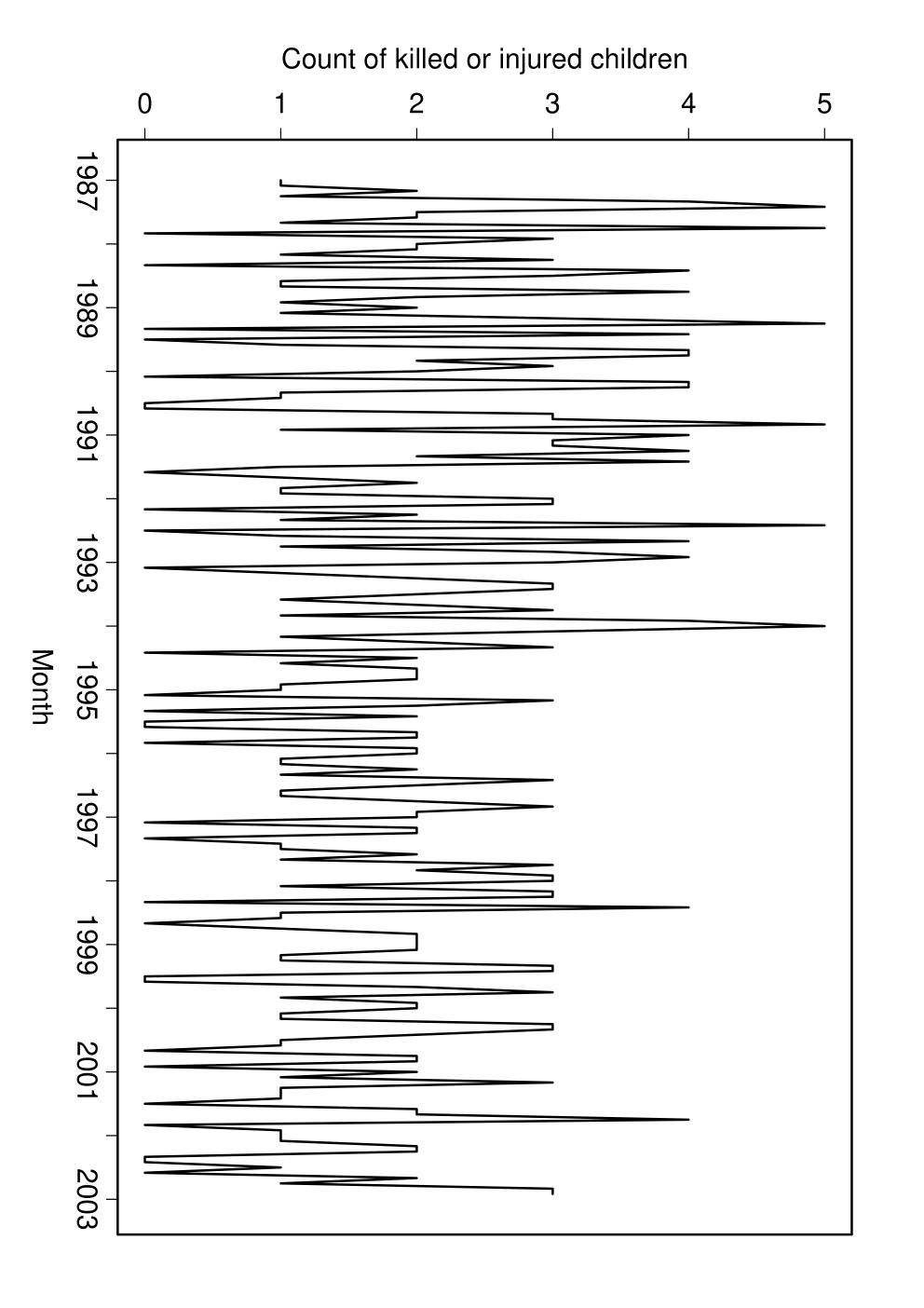
Table 7 presents the results of a Monte Carlo study using twelve replications with different random number seeds for the Poisson model. This simulation is based on the the first parallel computation method described in 3.1. The implementation details are given in appendix E.3. The table shows that the inefficiencies of the adaptive random walk Metropolis are at least seven times as large as those of the adaptive independent Metropolis Hastings.
| Ac. Rate | Min. Inef. | Median Inef. | Max. Inef. | Median ECT | ||||||
| Algorithm | Median | IR | Median | IR | Median | IR | Median | IR | Median | IR |
| Standard Particle Filter | ||||||||||
| RWM3C | 25.71 | 1.88 | 40.61 | 5.22 | 56.41 | 6.11 | 81.04 | 9.57 | 14.54 | 1.44 |
| IMH-MN | 40.90 | 5.23 | 4.15 | 0.88 | 6.04 | 2.56 | 15.90 | 29.70 | 1.55 | 0.66 |
| Auxiliary Particle Filter | ||||||||||
| RWM3C | 27.12 | 1.77 | 40.38 | 7.52 | 55.94 | 5.27 | 80.31 | 22.59 | 21.76 | 2.09 |
| IMH-MN | 41.78 | 3.80 | 4.16 | 0.72 | 6.47 | 2.14 | 22.03 | 28.13 | 2.43 | 0.74 |
We compared the eight models given in table 8 using marginal likelihood. All the models with seasonal effects include five harmonics. The table shows that the simplest model is slightly better than the level and intervention model which is consistent with the results reported in Frühwirth-Schnatter and Wagner (2006). However, the intervention parameter is clearly negative with high probability and two of the seasonal coefficients have high probability of being different from zero (results not shown). The bridge and importance samplers give similar estimates of the marginal likelihoods.
| Standard Particle Filter | Auxiliary Particle Filter | |||
|---|---|---|---|---|
| Poisson model | ||||
| Level | -320.984 | -320.987 | -320.995 | -320.995 |
| Level and trend | -333.110 | -333.122 | -333.100 | -333.100 |
| Level and intervention | -321.279 | -321.278 | -321.285 | -321.291 |
| Level, trend and intervention | -333.867 | -333.866 | -333.861 | -333.857 |
| Level and seasonality | -328.438 | -328.436 | -328.451 | -328.444 |
| Level, trend and seasonality | -343.214 | -343.202 | -343.246 | -343.247 |
| Level, intervention and seasonality | -328.632 | -328.640 | -328.662 | -328.657 |
| Level, trend, intervention and seasonality | -341.253 | -341.246 | -341.267 | -341.264 |
We also ran a simulation using the second parallel computing method described in section 3.1 with 20 000 iteration of the adaptive independent Metropolis Hastings sampler running on eight processors. Implementation details are in appendix E.3. Table 9 summarizes the results and shows that the ECT of the adaptive random walk Metropolis algorithm is nearly 50 times larger than the ECT of the adaptive independent Metropolis Hastings algorithm.
| Ac. Rate | Min. Inef. | Median Inef. | Max. Inef. | Median ECT | ||||||
|---|---|---|---|---|---|---|---|---|---|---|
| Algorithm | Median | IR | Median | IR | Median | IR | Median | IR | Median | IR |
| RWM3C | 26.37 | 0.86 | 40.60 | 7.57 | 56.41 | 4.40 | 85.81 | 26.95 | 107.70 | 13.41 |
| IMH-MN | 40.07 | 4.41 | 4.54 | 0.81 | 6.86 | 2.99 | 27.26 | 38.01 | 1.90 | 0.81 |
4.3.2 Sydney asthma data
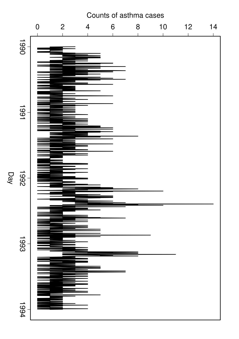
This example models the time series of daily counts of asthma presentations at the accident and emergency department of Campbelltown Hospital located in southwest metropolitan area of Sydney. figure 3 is a plot of the data, which has 1461 observations from January 1, 1990 to December 31, 1994. Davis et al. (2003) analyze this data using a Poisson model. Davis et al. (2003) argue that the peaks in the series can be lined up with the four terms in the school year with the break between the first and second terms occurring at varying times because of the timing of the Easter vacation. They include only one harmonic, to model the seasonal effect, and model the peaks by constructing the explanatory variable
where is the start time for the th school term in year and (a beta density), with parameter and . There are sixteen such explanatory variables but their preliminary analysis only includes eight of them corresponding to terms 1 and 2 across all four years. They also include the following explanatory variables: Sunday and Monday effects (dummy variables), maximum daily ozone, maximum daily NO2 and humidity.
We apply model (15) to the asthma data, but without the intervention variable, i.e. taking identically zero, and use the hyperparameters , , , , , , , , which are obtained through an empirical analysis of the data. Table 10 presents the results of a Monte Carlo study using twelve replications with different random number seeds for the Poisson model with level, trend and seasonality, and the explanatory variables. This simulation is based on the first parallel computation method described in 3.1, with the implementation details given in appendix E.4. The table shows that the inefficiencies of the adaptive random walk Metropolis are at least twice as large as those of the adaptive independent Metropolis Hastings.
| Ac. Rate | Min. Inef. | Median Inef. | Max. Inef. | Median ECT | ||||||
| Algorithm | Median | IR | Median | IR | Median | IR | Median | IR | Median | IR |
| Standard Particle Filter | ||||||||||
| RWM3C | 25.59 | 1.09 | 68.46 | 7.00 | 88.50 | 2.81 | 119.74 | 16.62 | 148.59 | 5.18 |
| IMH-MN | 27.52 | 7.75 | 8.51 | 6.18 | 16.45 | 15.62 | 52.26 | 49.66 | 27.73 | 26.34 |
| General Auxiliary Particle Filter | ||||||||||
| RWM3C | 26.52 | 3.45 | 73.96 | 8.06 | 87.41 | 1.64 | 114.99 | 14.29 | 219.95 | 4.26 |
| IMH-MN | 18.45 | 7.22 | 14.52 | 7.32 | 26.16 | 11.38 | 55.21 | 16.44 | 66.03 | 28.71 |
Table 11 uses marginal likelihood to compare the model with just the level in the transition equation to a model containing the level and the trend , with the simpler model preferred.
| Standard Particle Filter | Auxiliary Particle Filter | |||
|---|---|---|---|---|
| Model | ||||
| Level and seasonality | -2558.3 | -2558.3 | -2558.2 | -2558.3 |
| Level, trend and seasonality | -2577.3 | -2577.3 | -2577.2 | -2577.2 |
Acknowledgment
The research of Robert Kohn and Ralph S. Silva was partially supported by an ARC Discovery Grant DP0667069. We thank Professor Sylvia Frühwirth-Schnatter for the Linz data and Professor William T. M. Dunsmuir for the asthma data.
References
- Andrieu and Doucet (2002) Andrieu, C. and Doucet, A. (2002), “Particle filtering for partially observed Gaussian state space models,” Journal of the Royal Statistical Society, Series B, 64, 827–836.
- Andrieu et al. (2010) Andrieu, C., Doucet, A., and Holenstein, R. (2010), “Particle Markov chain Monte Carlo methods,” Journal of the Royal Statistical Society, Series B, 72, 1–33.
- Anscombe (1948) Anscombe, F. J. (1948), “The transformation of Poisson, Binomial and Negative-Binomial data,” Biometrika, 35, 246–254.
- Atchadé and Rosenthal (2005) Atchadé, Y. and Rosenthal, J. (2005), “On adaptive Markov chain Monte Carlo algorithms.” Bernoulli, 11, 815–828.
- Cappé and Rydén (2005) Cappé, O., M. E. and Rydén, T. (2005), Inference in Hidden Markov Models, New York: Springer.
- Chen and Shao (1997) Chen, M. H. and Shao, Q. M. (1997), “On Monte Carlo methods for estimating ratios of normalizing constants,” The Annals of Statistics, 25, 1563–1594.
- Davis et al. (2003) Davis, R. A., Dunsmuir, W. T. M., and Streett, S. B. (2003), “Observation-driven models for Poisson counts,” Biometrika, 90, 777–790.
- Del Moral (2004) Del Moral, P. (2004), Feynman-Kac Formulae: Genealogical and Interacting Particle Systems with Applications, New York: Springer.
- Del Moral et al. (2006) Del Moral, P., Doucet, A., and Jasra, A. (2006), “Sequential Monte Carlo samplers,” Journal of the Royal Statistical Society Series B, 68, 411–436.
- Doucet et al. (2001) Doucet, A., de Freitas, N., and Gordon, N. (2001), Sequential Monte Carlo Methods in Practice, New York: Springer.
- Doucet et al. (2000) Doucet, A., Godsill, S., and Andrieu, C. (2000), “On sequential Monte Carlo sampling methods for Bayesian filtering,” Statistics and Computing, 10, 197–208.
- Fearnhead and Clifford (2003) Fearnhead, P. and Clifford, P. (2003), “On-line inference for hidden Markov models via particle filters,” Journal of the Royal Statistical Society Series B, 65, 887–899.
- Flury and Shephard (2008) Flury, T. and Shephard, N. (2008), “Bayesian inference based only on simulated likelihood: particle filter analysis of dynamic economic models,” http://www.economics.ox.ac.uk/Research/wp/pdf/paper413.pdf.
- Frühwirth-Schnatter and Wagner (2006) Frühwirth-Schnatter, S. and Wagner, H. (2006), “Auxiliary mixture sampling for parameter-driven models of time series of counts with applications to state space modelling,” Biometrika, 93, 827–841.
- Galassi et al. (2009) Galassi, M., Davies, J., Theiler, J., Gough, B., Jungman, G., Alken, P., B. M., and Rossi, F. (2009), GNU Scientific Library Reference Manual, 3rd ed., http://www.gnu.org/software/gsl/.
- Geweke (1989) Geweke, J. (1989), “Bayesian inference in econometric models using Monte Carlo integration,” Econometrica, 57, 1317–1339.
- Giordani and Kohn (2010) Giordani, P. and Kohn, R. (2010), “Adaptive Independent Metropolis-Hastings by Fast Estimation of Mixture of Normals,” Journal of Computational and Graphical Statistics, available at http://ssrn.com/abstract=1082955.
- Gordon et al. (1993) Gordon, N. J., Salmond, D. J., and Smith, A. F. M. (1993), “A novel approach to non-linear and non-Gaussian Bayesian state estimation,” Radar and Signal Processing, IEE Proceedings F, 140, 107–113.
- Haario et al. (2001) Haario, H., Saksman, E., and Tamminen, J. (2001), “An adaptive Metropolis algorithm,” Bernoulli, 7, 223–242.
- Kim and Chib (1998) Kim, S., S. N. and Chib, S. (1998), “Stochastic volatility: Likelihood inference and comparison with ARCH models,” Review of Economic Studies, 65, 361–393.
- Kitagawa (1996) Kitagawa, G. (1996), “Monte Carlo filter and smoother for non-Gaussian non-linear state space models,” Journal of Computational and Graphics Statistics, 5, 1–25.
- Liu and Chen (1998) Liu, J. S. and Chen, R. (1998), “Sequential Monte Carlo methods for dynamic systems,” Journal of the American Statistical Association, 93, 1032–1044.
- Malik and Pitt (2008) Malik, S. and Pitt, M. K. (2008), “Modeling Stochastic Volatility with Leverage and Jumps: A ‘Smooth’ Particle Filtering Approach,” Available at http://www.riksbank.com/upload/Research/Conferences/StateSpace2008/Pitt.pdf.
- McDonald and Zucchini (1997) McDonald, I. and Zucchini, W. (1997), Hidden Markov and Other Models for Discrete-Valued Time Series, London: Chapman & Hall/CRC.
- Meng and Wong (1996) Meng, X. L. and Wong, W. H. (1996), “Simulating ratios of normalizing constants via a simple identity: A theoretical exploration,” Statistica Sinica, 6, 831–860.
- Pitt (2002) Pitt, M. K. (2002), “Smooth particle filters for likelihood evaluation and maximization,” .
- Pitt and Shephard (1999) Pitt, M. K. and Shephard, N. (1999), “Filtering via simulation: Auxiliary particle filters,” Journal of the American Statistical Association, 94, 590–599.
- Pitt and Walker (2005) Pitt, M. K. and Walker, S. G. (2005), “Constructing stationary time series models using auxiliary variables with applications,” Journal of the American Statistical Association, 100, 554–564.
- Polson et al. (2008) Polson, N. G., Stroud, J. R., and Müller, P. (2008), “Practical filtering with sequential parameter learning.” Journal of the Royal Statistical Society, Series B, 70, 413–428.
- Roberts et al. (1997) Roberts, G. O., Gelman, A., and Gilks, W. R. (1997), “Weak convergence and optimal scaling of random walk Metropolis algorithms.” Annals of Applied Probability, 7, 110–120.
- Roberts and Rosenthal (2007) Roberts, G. O. and Rosenthal, J. S. (2007), “Coupling and ergodicity of adaptive MCMC,” Journal of Applied Probability, 44, 458–475.
- Roberts and Rosenthal (2009) — (2009), “Examples of adaptive MCMC,” Journal of Computational and Graphical Statistics, 18, 349–367.
- Shephard (2005) Shephard, N. (2005), Stochastic Volatilty: Selected Readings, Oxford: Oxford University Press.
- Shephard and Pitt (1997) Shephard, N. and Pitt, M. (1997), “Likelihood analysis of non-Gaussian measurement time series,” 84, 653–667.
- Storvik (2002) Storvik, G. (2002), “Particle filters for state-space models with the presence of unknown static parameters,” IEEE Transactions on Signal Processing, 50, 281–290.
- Tierney (1994) Tierney, L. (1994), “Markov Chains for Exploring Posterior Distributions,” Annals of Statistics, 22, 1701–1728.
- Walker (1977) Walker, A. J. (1977), “An efficient method for generating discrete random variables with general distributions,” ACM Transactions on Mathematical Software, 3, 253–256.
- West and Harrison (1997) West, M. and Harrison, J. (1997), Bayesian Forecasting and Dynamic Models, New York: Springer-Verlag, 2nd ed.
Appendix A Standard particle filter
This section outlines the standard Sampling-Importance-Resampling (SIR) particle filter of Gordon et al. (1993). We suppress the dependence on the fixed parameter for notational convenience. Suppose that that we have samples for . The particle filter works by taking this sample, from the filtering density at time , and translating it into a sample from the filtering density at time . The first step involves simply passing each of these samples through the transition density to obtain , for , which produces samples which are approximately distributed from equation (1a). These samples are therefore samples from the prediction density (we denote filtered samples as and the corresponding predictive samples as ). To each of these samples, for , we attach the following weights, and corresponding masses,
| (16) |
This collection is now a discrete approximation to the filtering density . Explicitly, we may write this approximation, in terms of Dirac-delta functions, , as,
| (17) |
We need to resample from this mass function to obtain an equally weighted sample. However, prior to doing this we may estimate the term (1c) unbiasedly (Del Moral, 2004) by the denominator at equation (16),
| (18) |
We may also estimate any moments under the filtering density, say , in the Rao-Blackwellised form as,
Typically these estimators are more efficient than using the resampled analogs.
To produce an equally weighted sample from equation (17), we need only think about the sampling of the discrete univariate index with mass for . This is a multinomial sample and is the equivalent of a weighted bootstrap.22 2 The SIR filter is sometimes referred to as the bootstrap filter for this reason. We then have a sample of resampled indices. Having sampled in this manner, we can now associate our resampled points, which we call for , with the predictive points,
The method now proceeds to the next time step in a similar fashion.
We may replace the multinomial resampling (weighted bootstrap) procedure with a stratified sampling step instead. This does not affect the validity of the particle filter or the subsequent MCMC strategy that we pursue.
Appendix B Proof of theorem 2
This section briefly outlines the conditions for theorem 2 to hold and its proof. The generic auxiliary particle filter of Pitt and Shephard (1999) uses an importance density of the form , where is a suitable value of . We replace the term in the importance density by where is defined in theorem 1. By Pitt (2002), the term (1c) is estimated unbiasedly by
It follows that . The rest of the proof is the same as that of Theorem 1.
Appendix C Adaptive sampling schemes
This appendix describes the two adaptive sampling schemes used in the paper.
C.1 Adaptive random walk Metropolis
The adaptive random walk Metropolis proposal of Roberts and Rosenthal (2009) is
| (19) |
where is the dimension of and is a multivariate dimensional normal density in with mean and covariance matrix . In (19), for , with representing the initial iterations, for with ; is a constant covariance matrix, which is taken as the identity matrix by Roberts and Rosenthal (2009) but can be based on the Laplace approximation or some other estimate. The matrix is the sample covariance matrix of the first iterates. The scalar is meant to achieve a high acceptance rate by moving the sampler locally, while the scalar is considered to be optimal (Roberts et al., 1997) for a random walk proposal when the target is a multivariate normal. We note that the acceptance probability (3) for the adaptive random walk Metropolis simplifies to
| (20) |
We refine the two component random walk Metropolis proposal in (19) by adding a third component with and with . We take if , for and . We refer to this proposal as the three component adaptive random walk. The purpose of the heavier tailed third component is to allow the sampler to explore the state space more effectively by making it easier to leave local modes.
C.2 A proposal density based on a mixture of normals
The proposal density of the adaptive independent Metropolis-Hastings approach of Giordani and Kohn (2010) is a mixture with four terms of the form
| (21) |
with the parameter vector for the density . The sampling scheme is run in two stages, which are described below. Throughout each stage, the parameters in the first two terms are kept fixed. The first term is an estimate of the target density and the second term is a heavy tailed version of . The third term is an estimate of the target that is updated or adapted as the simulation progresses and the fourth term is a heavy tailed version of the third term. In the first stage is a Gaussian density constructed from a preliminary run, of the three component adaptive random walk. Throughout, has the same component means and probabilities as , but its component covariance matrices are ten times those of . The term is a mixture of normals and is also a mixture of normals obtained by taking its component probabilities and means equal to those of , and its component covariance matrices equal to 20 times those of . The first stage begins by using and only with, for example, and , until there is a sufficiently large number of iterates to form . After that we set and . We begin with a single normal density for and as the simulation progresses we add more components up to a maximum of six according to a schedule that depends on the ratio of the number of accepted draws to the dimension of .
In the second stage, is set to the value of at the end of the first stage and and are constructed as described above. The heavy-tailed densities and are included as a defensive strategy to get out of local modes and to explore the sample space of the target distribution more effectively.
It is computationally too expensive to update (and hence ) at every iteration so we update them according to a schedule that depends on the problem and the size of the parameter vector.
Appendix D Marginal likelihood evaluation using bridge and importance sampling
Suppose that is an approximation to which can be evaluated explicitly. Bridge sampling (Meng and Wong, 1996) estimates the marginal likelihood as follows. Let
where is a positive constant. Let
| (22) | ||||
Suppose the sequence of iterates is generated from the posterior density and a second sequence of iterates is generated from . Then
are estimates of and and is the bridge sampling estimator of the marginal likelihood .
In adaptive sampling, is the mixture of normals proposal. Although can be any positive constant, it is more efficient if is a reasonable estimate of . One way to do so is to take , where is the posterior mean of obtained from the posterior simulation.
An alternative method to estimate of the marginal likelihood is to use importance sampling based on the proposal distribution (Geweke, 1989; Chen and Shao, 1997). That is,
Since our proposal distributions have at least one heavy tailed component, the importance sampling ratios are likely to be bounded and well-behaved, as in the examples in this paper.
Appendix E Implementation details and sampling schedules
We coded most of the algorithms in MATLAB, with a small proportion of the code written using C/Mex files. For the particle filters, we also use a C/Mex file for the resampling step using an efficient algorithm to draw from a general discrete distribution (Walker, 1977) available as a C function in the GNU Scientific Library (Galassi et al., 2009). We carried out the estimation on an SGI cluster with 42 compute nodes. Each of them is an SGI Altix XE320 with two Intel Xeon X5472 (quad core 3.0GHz) CPUs with at least 16GB memory. We ran parallel jobs using up to eight processors and MATLAB 2009.
E.1 Implementation details for the S&P 500 index data
This section gives the implementation details for the first and second simulations in section 4.1.1. The first simulation uses a sampling rate of particles for each time period for each of eight processor, so each step of the particle filter uses 24 000 particles. The number of iterations of the adaptive samplers is 10 000 with the updates of the proposal distributions for the adaptive independent Metropolis-Hastings samplers performed at iterations 100, 200, 500, 1 000, 2 000, 3 000, 4 000, 5 000, 6 000 and 7 500. The adaptive independent Metropolis Hastings sampling scheme is initialized using 2000 iterations of the ARWM3C. The initial proposal for all the AIMH algorithms are based on a multivariate normal distribution estimated from these draws and the initial starting values are the sample means.
The second simulation uses eight processors with block sizes for each processor of 15, 25, 60, 125, 250, 375, 500, 625, 750 and 940, corresponding to 120, 200, 480, 1 000, 2 000, 3 000, 4 000, 5 000, 6 000 and 7 520 proposed parameter values before each update of the proposal density. The proposal distribution is updated at the completion of each block. In this simulation for the standard particle filter.
E.2 Implementation details for the weekly homicide data
This section gives the implementation details for the first and second simulations in section 4.2.1. The sampling rate for the first simulation is particles on each of eight parallel processors, so each step of the particle filter uses 24 000 particles. The number of iterations of the adaptive sampling algorithms is set to 10 000 with the updates of the proposal distributions for the adaptive independent Metropolis-Hastings samplers performed at iterations 100, 200, 500, 1 000, 2 000, 3 000, 4 000, 5 000, 6 000, and 7 500. The simulation is initialized as in E.1.
The schedule for the second simulation is the same as in section E.1.
E.3 Implementation details for the analysis of the Linz data
This section gives the implementation details for the first and second simulations in section 4.3.1. The sampling rate for the first simulation is particles in each of eight parallel processors. The number of iterations is 20 000 with updates of the proposal distribution for the adaptive independent Metropolis-Hastings sampler performed at iterations 300, 1 000, 3 000, 5 000, 10 000, and 15 000. The simulation is initialized as in E.1.
For the second simulation the number of iterations of the adaptive samplers is 20 000 with the adaptive independent Metropolis-Hastings sampler running on eight processors with the block sizes for each processor 40, 125, 375, 625, 1250, and 1875, corresponding to 320, 1000, 480, 3 000, 5 000, 10 000 and 15 000 proposed parameter values. The updates of the proposal distribution occur at the end of each block. In this simulation, particles for the standard particle filter.
E.4 Implementation details for analysis of the asthma data
This section gives the implementation details for the simulation in section 4.3.2. The sampling rate for the simulation is particles in each of eight parallel processes. The number of iterations is set to 50 000 with the updates of the proposal distributions for the adaptive independent Metropolis-Hastings samplers performed at iterations 1 000, 2 000, 3 000, 4 000, 5 000, 7 000, 8 000, 10 000, 15 000, 20 000, 25 000, 30 000, and 40 000.