A detailed investigation of the properties of a Vlasov-Maxwell equilibrium for the force-free Harris sheet
Abstract
A detailed discussion is presented of the Vlasov-Maxwell equilibrium for the force-free Harris sheet recently found by Harrison and Neukirch (Phys. Rev. Lett. 102, 135003, 2009). The derivation of the distribution function and a discussion of its general properties and their dependence on the distribution function parameters will be given. In particular, the distribution function can be single-peaked or multi-peaked in two of the velocity components, with possible implications for stability. The dependence of the shape of the distribution function on the values of its parameters will be investigated and the relation to macroscopic quantities such as the current sheet thickness will be discussed.
pacs
52.20.-j, 52.25.Xz, 52.55.-s, 52.65.FfI Introduction
Force-free plasma equilibria with the property
| (1) |
are of great importance, in particular for space and astrophysical plasmas. Equation (1) implies that the current density, , is parallel to the magnetic field, , so that it can be written as . In general, the function can vary with position, but has to be constant along magnetic field lines, since together with implies that
| (2) |
Obviously Eq. (2) is also satisfied if constant. This case is usually referred to as the linear force-free case, because the equation determining the magnetic field is linear in this case. Magnetic fields for which varies from field line to field line are called nonlinear force-free fields.
Whereas many force-free equilibria can be found using magnetohydrodynamics (MHD), this is not the case when Vlasov-Maxwell (VM) theory is used. Collisionless force-free equilibria have only been found for the special case where the magnetic field depends only on one spatial Cartesian coordinate (in this paper taken to be ). This case is trivial in MHD, but finding the appropriate distribution functions for given magnetic field and current density profiles for a collisionless equilibrium is a highly nontrivial task. The reason for this difficulty is that one has to try and solve the VM problem in the opposite direction than it is usually treated, which is to specify the distribution functions (DFs) and then to calculate the magnetic field by solving Ampère’s law.
This difficulty is reflected by the fact that only a very small number of exact force-free VM equilibrium DFs are known and all known solutions were of the linear force-free type[1, 2, 3, 4] until the first nonlinear force-free VM equilibrium DF was presented in a recent Letter.[5] The DFs found in Ref. 5 are for the force-free Harris sheet, with a magnetic shear field ensuring force balance instead of a plasma pressure gradient as in the original Harris sheet.[6]
For reasons of space no detailed discussion of a) the derivation of the DFs and b) their properties has been given in Ref. 5. In the present publication, we aim to give a full discussion of the method used to derive the DFs in Sect. II and of its properties in Sect. III. Of particular interest is the possibility that the DFs can have multiple maxima in two of the velocity components (in the coordinate system used in this paper the - and -components), which may have stability implications. Therefore, a detailed investigation of the connection between the shape of the distribution function and the parameter values was carried out. A summary and conclusion will be presented in Sect. IV.
II Calculation of the equilibrium distribution function
II.1 Basics
We use Cartesian coordinates , , complemented by the corresponding velocities , , for the DFs. We assume spatial invariance in and , i.e. all quantities depend only upon . We also assume time-independence.
For the problems considered in the present paper the magnetic field has only two non-vanishing components, and , which, using an appropriate gauge, can be written in terms of a vector potential in the form
| (3) |
| (4) |
The electric field is given by the negative gradient of an electric potential such that
| (5) |
The magnetic and electric fields thus automatically satisfy the homogeneous steady-state Maxwell equations and .
Due to time independence and spatial symmetries we have three obvious constants of motion for particles of species with charge and mass moving in these fields, namely the particle energy, ,
| (6) |
the canonical momentum in the -direction, ,
| (7) |
and the canonical momentum in the -direction, ,
| (8) |
Solutions of the steady state Vlasov equation
| (9) |
are given by all positive functions depending only on the constants of motion,
| (10) |
and satisfying the appropriate conditions for existence of the velocity moments. If the same combination of values for the constants of motion allows particle trajectories in several distinct regions of phase space then it is in principle possible to assign different values to in each region[7, 8], but this possibility will not be considered in the present paper (for an example of 2D rotationally symmetric VM equilibria see e.g. Ref. 9).
Using the assumption of quasineutrality to determine the electric potential , one can show[8, 10] that the VM equilibrium problem reduces to solving Ampère’s law in the form
| (11) | |||||
| (12) |
where
| (13) |
is the -component of the plasma pressure tensor.
It is obvious (see e.g. Ref 10) that Eqs. (11) and (12) are equivalent to the equations of motion of a particle in a 2D conservative potential, with taking the role of time, and the coordinates of the particle and being the potential. As in the analogous particle problem one can integrate Eqs. (11) and (12) once to get
| (14) |
so that
| (15) |
i.e. the total pressure (magnetic plus plasma pressure) is constant for this class of VM equilibria. The total pressure corresponds to the total energy in the particle problem.
Knowledge of the shape of can provide insight into the nature of the solutions of Eqs. (11) and (12) in the same way as knowledge of the potential as a function of position in the equivalent particle problem can provide information about the nature of the possible trajectories of the particle. It is usually straightforward to calculate as a function of and if the equilibrium DFs are specified. It may, however, also be possible to determine equilibrium DFs for a given function using a method suggested by Channell.[2]
II.2 Channell’s Method
To be able to make analytical progress in determining a distribution function from a number of assumptions have to be made. The first assumption made is that the dependence of the DFs on the Hamiltonian is of the form of a negative exponential, i.e
| (16) |
with , and an unknown function of the canonical momenta. Using this DF becomes
| (17) |
with
| (18) |
The charge density, , can be calculated by taking the negative derivative of with respect to the electric potential[8, 10] as
| (19) |
Assuming a two-species plasma with both species having the same charge with opposite sign (e.g. electrons and protons) and quasi-neutrality by letting , one can determine the quasi-neutral electric potential to be
| (20) |
Channell’s[2] final assumption is strict neutrality, i.e. that for all possible values of , , implying that . This will impose additional conditions on the parameters of the DFs which have to be satisfied, but this is in principle not a problem.
The neutral is then given by
| (21) |
Using the canonical momenta instead of the velocity components as integration variables and using Eq. (21), Eq. (18) becomes
| (22) | |||||
For a known function of and , this is a Fredholm integral equation of the first type for the unknown function . The kernel of this integral equation
| (23) |
depends only upon the difference of its arguments and the standard method for solving such integral equations is using Fourier transforms, as also suggested by Channell.[2]
It must, however, be pointed out that to be able to determine by Fourier transforms two conditions need to be satisfied: a) the Fourier transform of must exist and b) the inverse Fourier transform to obtain must exist. Especially condition b) can prove difficult to meet as the inverse Fourier transform involves a factor with the inverse of the Gaussian in the convolution integral, i.e. an exponential function with a positive quadratic argument. Channell[2] treats several examples for which the Fourier transform method does not work using other methods. For the force-free Harris sheet case discussed in the present paper, we will also use a more direct method to solve Eq. (22) because Fourier transforms are only of limited applicability to our case and because the other method turns out to be more instructive.
II.3 Harris sheet and force-free Harris sheet
The Harris sheet[6] is a well-known one-dimensional VM equilibrium. It is widely used in theoretical plasma physics, for example for reconnection studies, because it is a typical neutral current sheet and is mathematically well-behaved. The magnetic field is given by
| (24) |
the current density by
| (25) |
and the vector potential (in a convenient gauge) by
| (26) |
Force balance is maintained by a pressure gradient with given by
| (27) |
with and a constant background pressure. The distribution function used by Harris[6] is given by
| (28) |
which is a Maxwellian DF in all velocity directions, but with a constant average bulk flow velocity of in the -direction. Other distribution functions giving rise to the same magnetic field and pressure profiles have also been found (see e.g. Ref. 11). By using either the distribution function (28) directly or Eqs. (26) and (27), one can show that
| (29) |
Note that to get a constant background pressure from the distribution function an extra term proportional to has to be added to the right-hand side of Eq. (28). Using that the equilibrium condition (15) is satisfied with
| (30) |
The force-free Harris sheet has the same as the Harris sheet, but is kept in force balance by magnetic pressure due to a component, with being constant. The magnetic field is then given by
| (31) |
The current density is
| (32) |
with where
| (33) |
The vector potential, again in a convenient gauge, is given by
| (34) |
At this point, no form for as a function of and and no DF are known for this equilibrium magnetic field. The derivation of both will be discussed in the next section. Plots of the magnetic field components, current density and pressure as functions of are shown in Fig. 1.


.
II.4 Derivation of the distribution function
To be able to apply Channell’s method to find a DF for the force free Harris sheet, we first need to find an appropriate function for these cases. It can be shown[10] that to find a that allows a force-free solution is equivalent to finding a potential for which at least one of its equipotential lines is identical with a particle trajectory. The simplest examples for this are attractive central potentials whose contours are circles and which also allow circular orbits. The corresponding 1D VM equilibria are linear force-free magnetic fields.[1, 2, 3, 4]
It is obvious, however, that the for the force-free Harris sheet has to be more complex than a central potential. The approach chosen in Ref. 5 was to let
| (35) |
In this case the Eqs. (11) and (12) decouple and can be integrated separately. Thus one can see immediately that is identical to given by Eq. (29). The unknown function can be determined from inverting using Eq. (34) and substituting into
| (36) |
Using the trigonometric identity
| (37) |
one can see that
| (38) |
so that, dropping the subscript ,
| (39) |
Using and putting together and , we arrive at the form of given in Ref. 5
| (40) |
where . By construction, Ampère’s law (11) and (12) generated from this has the vector potential (34) as a solution, and this solution coincides with a contour of . In Fig. 2 we show a surface plot of for the force-free case with the vector potential for the force-free Harris sheet shown as a trajectory at the top of the plot.

Having found a , we can use Channell’s method[2] to find the corresponding DF. As the relation between the unknown function and is linear, it is immediately clear that must also have the form of a sum,
| (41) |
with
| (42) | |||||
| (43) |
For the time being we can ignore any constant parts of and , because the solution for a constant is simply a constant , which can be added at the end of the calculation due to the linearity of the problem.
For solving Eq. (42) with one could in principle use Fourier transforms, but we shall use a more direct method here. The method is based on the observation that, using the trigonometric identity , one has
| (44) |
Thus, rewriting the integral in Eq. (42) using as integration variable instead of , one can see immediately that a leads to a . The constant has the dimensions of a velocity so that the argument of the cosine function is dimensionless.
The solution to Eq. (43) is already known, because this part of the pressure gives rise to the -component of the current density and thus to the Harris sheet . Therefore, we must have (note that the case of a simple exponential is also a special case of one the examples in Channell’s paper[2]). This means that the part of the DF depending explicitly on is identical with the -dependent part of the original Harris sheet DF (28).
The full distribution function therefore has the general form
| (45) |
with , , and being constant parameters of the DF in addition to and . We remark that we assume that at this point to ensure that remains positive. The parameters of the DF will have to satisfy a number of consistency relations due to the assumptions made for applying Channell’s method and in order to relate the microscopic DF parameters to the macroscopic parameters and .
II.5 Consistency Relations
The pressure tensor component we obtain using Eq. (45) is of the general form (17) with
| (46) | |||||
The fundamental condition for Channell’s method to be applicable is . This is satisfied if
| (47) | |||||
| (48) | |||||
| (49) | |||||
| (50) | |||||
| (51) |
For the case of the original Harris sheet, Eq. (51) is well known[12] as the condition for a vanishing electric potential. In the Harris sheet case, is the constant average bulk velocity of species in the -direction and condition (51) is basically specifying a particular frame of reference. In the case of the force-free Harris sheet, the average bulk velocity for both the - and the -velocity components varies with and one thus needs more conditions, but in principle one can still interpret Eqs. (47) to (51) as conditions for a particular frame of reference in which the electric potential vanishes.
III Properties of the equilibrium distribution function
III.1 Relation between microscopic and macroscopic parameters
Although we have now derived the DF for the force-free Harris sheet, we have not yet related the set of microscopic parameters of the DF, namely , , , and , to the macroscopic parameters of the equilibria, which are and . The easiest way to find this connection is to compare Eq. (52) with Eq. (40). This leads to
| (53) | |||||
| (54) | |||||
| (55) | |||||
| (56) | |||||
| (57) |
where we have assumed that is positive, but allow for to be negative.
To make the connection with the original Harris sheet results we use Eqs. (57) and (53) to derive an expression for in the form (see also Ref. 12, Chapter 6)
| (58) |
which is symmetric in electron and ion parameters. Using Eq. (57), expressions for using only electron or only ion parameters can be derived from Eq. (58).
The relation of the other macroscopic parameters to the microscopic parameters are more obvious. Equation (53) directly relates , the magnetic field strength in the limit , with , and . In the original Harris sheet case, is the maximum value of the -dependent part of the particle density at , and Eq. (53) simply states that the magnetic pressure for has to be equal to the plasma pressure at due to force balance. As we will see later, in the force-free Harris sheet case the meaning of changes, but because we have effectively separated the total force-balance into two conditions for and , the same condition as for the original Harris sheet still applies for the force-free Harris sheet as well.
Equation (54) directly shows that for the force-free Harris sheet we have .
Equation (55) relates the constant background pressure to the microscopic parameter , which is representing the magnitude of the part of the DF which depends only on . Obviously, is simply the ratio of the background pressure to the pressure . Equation (56), together with Eq. (57), allows us to relate to by writing
| (59) |
An expression for for the force-free Harris sheet equilibrium which is symmetrical in electron and ion parameters is given by
| (60) |
with
| (61) |
An expression for which is symmetrical in ion and electron parameters is obtained by using (60) in Eq. (21). Using the vector potential for the force-free Harris sheet, (34), we obtain for the particle density as a function of , expressed using microscopic parameters,
| (62) |
the pressure is obtained by multiplying by .
The mean bulk flow velocities of each species in the - and -directions as functions of , namely
| (63) | |||||
| (64) |
which gives a current density of the form
| (65) | |||||
| (66) |
III.2 The number of maxima of the DF in and
One of the interesting features of the force-free Harris sheet DF (45) is that it can have multiple maxima in both the - and the -directions. We shall discuss the -direction first as it is simpler to understand. Looking at the structure of the DF in the direction one can immediately see that it consists of the Harris sheet DF part, which is a Maxwellian distribution function drifting with a constant velocity in the -direction, and a part which, if regarded purely as function of , is Maxwellian at rest. It is intuitively clear that one should get two maxima in if the drift velocity increases, because the drifting Maxwellian moves towards the tail of the Maxwellian at rest. As we show in appendix A it is relatively straightforward to work out that a necessary condition for having more than one maximum in the -direction is
| (68) |
i.e. the constant drift velocity has to be larger than twice the thermal velocity. There is, however, a second condition on the parameter that also needs to be satisfied for the DF to have more than one maximum in . We derive and state the exact condition in appendix A, but its physical meaning is very easy to understand. If exceeds a certain limiting value, the part of the DF which does have vanishing average velocity in the -direction dominates over the other part of the DF, so that a second maximum cannot develop even if (68) is satisfied. Usually, this condition on will not be very restrictive, though, as the upper limit for grows exponentially with (see appendix A). We show examples of DFs as functions of for the different cases in Figs. 3 - 5. For these figures the values of have been chosen to be close to the critical value discussed in appendix A for illustrative purposes. The values for are of the order for the examples shown, which corroborates the point made above regarding the exponential growth of the limiting value.


We now turn to the dependence of the DF on . Due to the cosine-dependence it is clear that the possibility of multiple maxima in exists. We discuss the details of the calculation in appendix B. From the analysis in appendix B we find that the condition for having just a single maximum in is
| (69) |
This condition on can be understood in the same way as the similar condition on derived for the -dependence. If is large enough the Maxwellian background plasma it represents dominates the part of the DF with the cosine dependence and we only have a single maximum of the distribution function. If the condition (69) is not satisfied then we have multiple maxima in , but their existence still depends on the values of and . Obviously, for small the limiting value on the right hand side of (69) is , which is consistent with the absolute lower limit on mentioned before. Examples of the different cases are shown in Figs. 6 to 8.


A slightly different perspective on the discussion above can be provided if we express the ratio in terms of the current sheet thickness . Using Eq. (57), we get
| (70) |
where is the thermal gyroradius of species . If all parameters except and are fixed, it is obvious that a decrease in the current sheet thickness will eventually lead to multiple maxima in the DF, first in by violating condition (69) and then in as well. This may obviously have implications for possible velocity instabilities of the system, e.g. the two-stream or bump-on-tail instabilities, apart from macroscopic instabilities of the current sheet, e.g. the collisionless tearing mode. A detailed investigation of the stability properties of this inhomogeneous Vlasov-Maxwell equilibrium would be very interesting, but is beyond the scope of the present paper and will be left for future work.
IV Summary and Conclusions
We have given a detailed presentation of the derivation and the properties of the DF for the collisionless force-free Harris sheet found in Ref. 5. In particular, we have shown how the microscopic parameters of the DF are related to the macroscopic parameters of the magnetic field. We have also given a detailed derivation of the conditions on the parameters of the DF to ensure that it has only a single maximum in and in . We have shown that as the current sheet thickness decreases the condition for multiple maxima will eventually be violated and we have suggested that this may lead to velocity space instabilities in addition to other macroscopic instabilities for thin current sheets. The stability properties of the VM equilibrium are a very interesting topic for further investigations.
Acknowledgements.
The authors acknowledge support by the UK’s Science and Technology Facilities Council and by the European Commission through the SOLAIRE Network (MTRN-CT-2006-035484).Appendix A Condition for two maxima in the -direction
From a mathematical point of view it is easier to write the DF as a function of the momenta when carrying out this calculation. The -dependence does not play any role in the calculation and can be integrated out. The reduced DF for and then reads
| (71) |
where , with , , , , and similarly .
For an extremum of in the direction the derivative
| (72) | |||||
must vanish, leading to the condition
| (73) |
We remark that the right hand side is well-defined because .
The left hand side of (73) is a linear function of unit slope in , which crosses the -axis at . As varies between and , the left hand side intercepts the -axis for negative values of . The right hand side of (73) can be rewritten as
| (74) |
where and . The function (74) is positive, increases monotonically and is bounded between and . Therefore, a necessary condition for multiple maxima of the DF in (or ) is that the maximum slope of must be larger than . Otherwise the (73) can only have a single solution, implying a single maximum for the distribution function. It is straightforward to show that has its maximum slope at . So the necessary condition for multiple maxima is which translates into
| (75) |
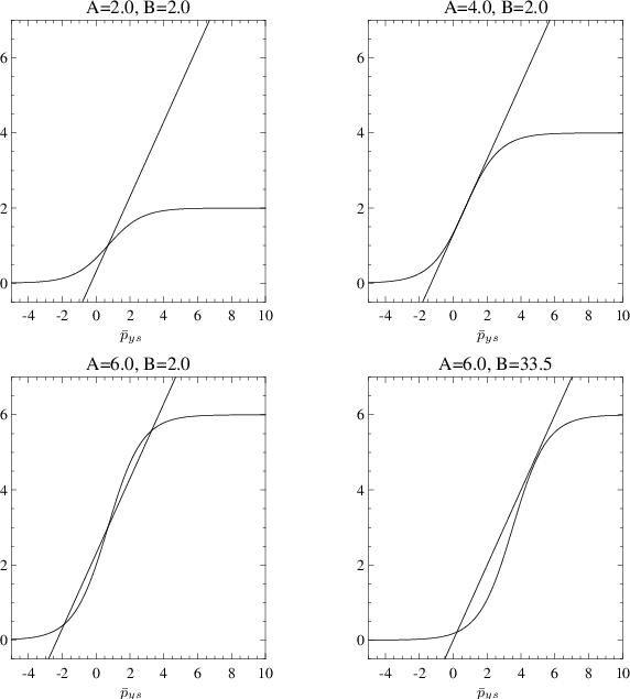
However, (75) is not sufficient, because even if it is satisfied, it is still possible that intersects with only once, namely if the value of is large enough. As discussed above the left hand side of (73) can only cross the -axis for , depending on the value of (and thus ). Since the is positive it can happen that takes on its maximum slope too far to the right for more than one intersection between the two functions to happen.The transition between three intersections to one intersection happens at the value of for which the straight line of slope one through the origin just touches the graph of at the point where it also has unit slope (see Fig. 9). One can easily calculate the value of for which the function has unit slope as
| (76) |
Two remarks are to be made here:
- •
only has a real value if , which is consistent with the condition found before for to have slope greater than unity anywhere;
- •
For , the function has unit slope at two values of , of which one has to choose the larger one (see Fig. 9), as we have done above.
The limiting value for can now derived from
| (77) |
leading to
| (78) |
so the sought for condition is
| (79) |
Since still depends upon we have to replace it by the minimum value it can take on as function of to get a condition which is independent of .
In summary, the DF has more than one maximum in (and thus in ) if the following conditions are both satisfied
| (80) | |||||
| (81) | |||||
where we have made use of (48) to replace .
Appendix B Condition for multiple maxima in the -direction
The analysis here is very similar to that in appendix A. Again we use the reduced DF (71) expressed as a function of the canonical momenta and . Taking the derivative of with respect to gives
| (82) | |||||
Setting this to zero gives the equation
| (83) |
or, in an abbreviated form
| (84) |
with
| (85) |
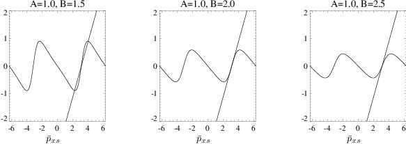
where and , because . The function (85) is a bounded periodic function of . Furthermore, varies between and , so the left hand side of (84) can only cross the -axis between and . The slope of is given by
| (86) |
which shows that has a positive slope for , which is always satisfied for some in the interval . Therefore, a necessary and sufficient condition for multiple maxima of the DF in is that has a maximum slope which is larger than unity. Examples for the different cases are shown in Fig. 10.
Taking the derivative of (86) we get
| (87) |
A brief calculation shows that has positive slope only for with an odd integer. The maximum value of the slope is given by , which leads to the condition
| (88) |
for the DF to have only one maximum. The lowest value can take (as a function of ) is so that we finally arrive at the condition
| (89) |
for the DF to have only one maximum in , where we have used (48) and (54) to replace .
References
- [1] A. Sestero, Physics of Fluids 10, 193 (1967).
- [2] P. J. Channell, Physics of Fluids 19, 1541 (1976).
- [3] N. A. Bobrova and S. I. Syrovatskiǐ, Soviet Journal of Experimental and Theoretical Physics Letters 30, 535 (1979).
- [4] N. A. Bobrova, S. V. Bulanov, J. I. Sakai, and D. Sugiyama, Physics of Plasmas 8, 759 (2001).
- [5] M. G. Harrison and T. Neukirch, Physical Review Letters 102, 135003 (2009a).
- [6] E. G. Harris, Nuovo Cimento 23, 115 (1962).
- [7] H. Grad, Physics of Fluids 4, 1366 (1961).
- [8] H. E. Mynick, W. M. Sharp, and A. N. Kaufman, Physics of Fluids 22, 1478 (1979).
- [9] T. Neukirch, Journal of Geophysical Research 98, 3753 (1993).
- [10] M. G. Harrison and T. Neukirch, Physics of Plasmas 16, 022106 (2009b).
- [11] W.-Z. Fu and L.-N. Hau, Physics of Plasmas 12, 070701 (2005).
- [12] K. Schindler, Physics of Space Plasma Activity (Cambridge, 2007).