Local likelihood estimation of local parameters for nonstationary random fields.

Stationary random fields play a fundamental role in both theoretical and applied spatial statistics. Unfortunately, stationarity is often violated when working with real data. The issue is more pressing with the recent data deluge and high resolution sensing where non-stationarity can be clearly visible. This presents a challenge for the spatial statistician who is interested in estimating and modeling dependency structure in random fields.

Even though stationarity is often criticized as being too simplistic, we believe it is still important for the understanding and development of nonstationary models. The reason is that any type of statistical estimation requires some sort of replication to “average over”. In spatial statistics the data often comprise of one realization of a random field. In this case, the assumption of stationarity provides a type of replication that makes statistical estimation possible. For nonstationary random fields, however, the lack of any assumption leads to a breakdown in statistical estimation due to the absence of replication. This problem can be mitigated by adding assumptions on the nonstationary random field like local stationarity, for example. The idea is that on small enough spatial scales, one hopes that the local dependency of the random field near a point is well approximated by some stationary random field. In this paper, we do not attempt a precise definition of local stationarity (see [4] for a definition in the time series literature). Instead, we take it for granted that such random fields exist (however one defines it) and enter into a discussion of how one might estimate the parameters of a local stationary approximation when observing a single realization of the nonstationary random field at dense (possibly uneven) observation locations. To accomplish these goals we develop a local likelihood approach for estimating local parameters.

Before we continue we mention why the standard local likelihood techniques fail for estimating the local dependency of a random field. In current techniques (see [5], for example), the independence structure of the data typically allow one to decompose the log-likelihood as a sum. Each summand depends on one data point, which can be down weighted as a function of some spatial covariate. In the random field case, however, there is no independence and therefore no such decomposition of the log-likelihood. A different technique that does work for random fields is to simply divide the observation locations into neighborhoods and fit a stationary random field model on each neighborhood. Typically two problems arise with this approach. First, the range of validity of a stationary approximation can be too small to contain enough data to estimate it. Second, it can produce non-smooth local parameter estimates, which can be undesirable in many cases.

In this paper we present an exposition through computation, simulation and some theory of our version of local likelihood estimation. A large portion of the paper is devoted to the discussion of different ways of constructing and estimating the weights used in our local likelihood that downweights the influence of distant observations of the random field. We start in Section 2 with our definition of a weighted local likelihood and then immediately apply it to the problem of variance modulation in Section 3. This example is convenient since the local likelihood estimate has a closed form and one can derive the Bayes risk under a polynomial prior for $\sigma(x)$. In Section 4 we study the problem of estimating the bandwidth parameter $\lambda$ from data. Finally, in Section 5 we apply these techniques to the estimation of the local fractional index of a local Matérn random field when observing one realization of the field at uneven observation locations in $\mathbb{R}^{2}$.

Before we present our notion of local likelihood it will be advantageous to set some notation. We write a random field as $\{Z(t)\colon t\in\mathbb{R}^{d}\}$ or just $Z$ when the domain of definition is clear from context. We distinguish two types of random field models: global and local. The only real distinction is nonstationary versus stationary but the nomenclature is useful since we regard global models as the true nonstationary sampling distribution and local models as the local stationary approximations. We consider global models that are nonstationary random fields indexed by some nonparametric function $\theta(t)$ that takes spatial arguments $t\in\mathbb{R}^{d}$ and returns values in some $m$-dimensional parameter space $\Theta\subset\mathbb{R}^{m}$. We call the function $\theta(\cdot)$ the local parameter function and denote resulting global model $G_{\theta(\cdot)}$. For each fixed $t_{0}\in\mathbb{R}^{d}$, the parameter vector $\theta_{0}=\theta(t_{0})$ determines a local random field model, denoted by $L_{\theta_{0}}$, which is generally stationary and models the stochastic behavior of $Z$ near some point $t_{0}$. Informally this means that $\mathcal{L}_{L_{\theta_{0}}}\{Z(t_{0}+h)\colon|h|<\epsilon\}\approx\mathcal{L}_{G_{\theta(\cdot)}}\{Z(t_{0}+h)\colon|h|<\epsilon\}$ when $\epsilon$ is small ($\mathcal{L}_{L_{\theta_{0}}}$ denotes the law of the finite dimensional distributions under model $L_{\theta_{0}}$). For the remainder of the paper a local parameter function will be denoted by $\theta(\cdot)$, $\theta(t)$ or just $\theta$ and a particular value in the parameter space $\Theta\subset\mathbb{R}^{m}$ will be written $\theta_{0}$.

For a concrete example, let $Z$ be a random field on $\mathbb{R}^{d}$ such that there exists a fixed but unknown function $\sigma(t)\colon\mathbb{R}^{d}\rightarrow\mathbb{R}^{+}$ and a known stationary random field $W$ such that $Z(t)=\sigma(t)W(t)$. In this case, $\sigma(t)$ is the local parameter function and $G_{\sigma(\cdot)}$ denotes the true distribution of $Z$. If $\sigma(t_{0}+h)\approx\sigma_{0}$ when $|h|$ is small then the local model for $Z$ at $t_{0}$, denoted by $L_{\sigma_{0}}$, is just the law of $\sigma_{0}W(t)$. Presumably if one has enough data in a neighborhood of $t_{0}$ one could successfully estimate $\sigma(t_{0})$ by fitting the model $L_{\sigma_{0}}$ to the data. Notice there is an inherent bias-variance tradeoff when fitting $L_{\sigma_{0}}$ locally to data: increasing the size of the local neighborhood reduces the variability of the estimate but increases the bias due to the inaccuracy of the stationary approximation. It is with local likelihoods that we seek to balance these two competing terms by smoothly down weighting the dependence of far away observations.

To define the local likelihood estimation of $\theta(\cdot)$ suppose we have $n$ observations $(t_{1},z_{1}),\ldots,(t_{n},z_{n})$ of a single realization of a random field $Z$ (the spatial locations are $t_{j}\in\mathbb{R}^{d}$ and the responses are $z_{j}=Z(t_{j})$). For any given location $t\in\mathbb{R}^{d}$, let $\mathcal{N}_{t,k}$ denote the set of $k$ observations nearest to $t$. Given weights $w_{1},\ldots,w_{n}$ (possibly depending on $t$, $t_{k}$ and a bandwidth parameter $\lambda$) we define the following weighted local likelihood:

where $\ell(\mathcal{N}_{t,k}|L_{\theta_{0}})$ is the log likelihood of the data in $\mathcal{N}_{t,k}$ under the model $L_{\theta_{0}}$ (note: we define $\ell(\mathcal{N}_{t,0}|L_{\theta_{0}})$ to be $0$). Now our local likelihood estimate of $\theta(t)$ is defined as

We first remark that if the weights $w_{k}=1$ for all $k$, then the telescoping sum in (1) collapses and one recovers the full likelihood for the local stationary model. Indeed $\mathcal{W}_{\lambda}$ orders and subsequently downweights the incremental changes in the stationary likelihood when adding the observations one by one in order of their distance to $t$. An important feature of the estimate $\hat{\theta}_{\lambda}$ is that, at least for Gaussian random fields, the computational cost of $\mathcal{W}_{\lambda}(\theta_{0},t|\text{data})$ is comparable to that of $\ell(\theta|\text{data})$ by either up dating a Cholesky decomposition or down dating an inverse covariance matrix. Moreover, the estimate $\hat{\theta}_{\lambda}(t)$ will typically be a “smooth” function of $t$ (when the weights are smooth) even when there is no natural additive or multiplicative structure on the parameter space $\Theta\subset\mathbb{R}^{m}$. Finally we remark that $\hat{\theta}_{\lambda}$ depends on the bandwidth parameter $\lambda$ through the weights $w_{k}$ which typically have the form $w_{k}\triangleq K((t-t_{k})/\lambda)$ for some smoothing kernel $K$.

We start with a particularly simple example, already mentioned in the previous section: estimating the local variance of a Gaussian random field. Consider the estimation of the function $\sigma(t)\colon\mathbb{R}\rightarrow\mathbb{R}^{+}$ when observing $\sigma(t)W(t)$ where $W$ a mean zero Gaussian process on $\mathbb{R}$ with known Matérn parameters. This example is useful since the local maximum likelihood estimate has a closed form solution. We take advantage of this solution by deriving the Bayes risk under polynomial priors. The Bayes risk is then used to give concrete evidence of a bias and variance trade for reducing estimation error. We also use the Bayes risk to explore the relationship between higher order kernels, bias of the resulting estimates and optimal bandwidth.

To derive the closed form solution of the local likelihood estimate we first need some notation. Let $\Sigma_{k}$ denote the covariance matrix of the observations in the $k$ neighborhood of $t$, i.e. $\mathcal{N}_{t,k}$, and let $\bm{z}_{k}\triangleq(z_{1},\ldots,z_{k})^{T}$ denote the responses of the data in $\mathcal{N}_{t,k}$. Notice that

and therefore

The maximum occurs at

which is the local maximum weighted likelihood estimate of $\sigma^{2}$ at $t$.

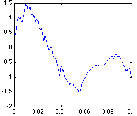
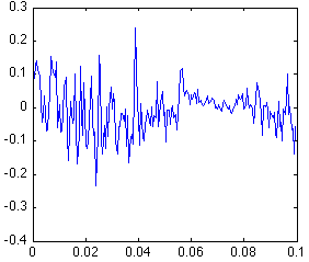
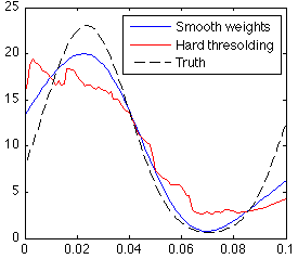
Figure 1 shows an example of this local likelihood estimate (blue line in the right-hand diagram) as compared with naïve local likelihood estimation (red line in the right-hand diagram) where the stationary model is presumed to hold through the local neighborhood. The left most diagram in Figure 1 shows the simulated field $\sigma(t)W(t)$ at $200$ evenly spaced observation locations in $[0,1]$, where $W$ is a mean zero Gaussian random field with known Matérn autocovariance function with parameters $(\sigma^{2},\nu,\rho)=(1,0.8,0.2)$ (using the parameterization given on page 50 of [14]) and unknown $\sigma(t)=2\sin(t/0.015)+2.8$. Notice that even though the local variance changes significantly throughout the observation region, it is difficult to see since the range parameter $\rho=0.2$ is relatively large compared with the observation region. However, if one looks at increments of $\sigma(t)W(t)$, shown in the middle diagram, the change in local variance becomes clearly visible. The true local parameter function $\sigma^{2}(t)$ is shown in the right hand plot of Figure 1 (dashed). The smooth weights take the form $w_{k}=K((t-t_{k})/\lambda)$ where $K$ is defined as $K(t)\triangleq e^{-t^{2}/2}(15-10t^{2}+t^{4})/8$ which is kernel $K_{6}$ presented in [17] (and also used in Section 3.1 below). The bandwidth used for both estimators is obtained by minimizing the Kullback-Leibler divergence of the estimated global model $G_{\hat{\sigma}^{2}_{\lambda}(\cdot)}$ to the truth at the observation locations. Notice that using smooth weights, the local likelihood estimate can not only reduce estimation error but can also yield smooth estimates of the local parameter function $\sigma^{2}$.

Remark: Although the computation of each $\Sigma_{k}^{-1}$ in (2) can be very time consuming, there is a downdating algorithm that makes all the inverses obtainable in nearly the same computational time as $\Sigma_{n}^{-1}$ (where $n$ is the number of observations). Once the inverse $\Sigma_{k}^{-1}$ is computed, the downdate $\Sigma_{k-1}^{-1}$ is easily computable by the following formula:

where $k=c-b^{T}\Sigma_{k-1}^{-1}b$. Therefore

where $\Sigma_{k}^{-1}{(a\colon\!b,c\colon\!d)}$ denotes the sub-matrix of $\Sigma_{k}^{-1}$ of rows $a$ through $b$ and columns $c$ through $d$. Note that the estimates $\hat{\sigma}^{2}(t)$ and $\hat{\sigma}^{2}(s)$ at two different locations $t\neq s$ are very similar: the only difference is the order one downdates the row and column of $\Sigma_{n}^{-1}$. This means one can construct $\hat{\sigma}^{2}$ at may different spatial locations by computing $\Sigma_{n}^{-1}$ once and for all, then downdate the inverse in different row and column orders.

The local likelihood estimates $\hat{\theta}_{\lambda}$ can vary dramatically depending on the choice of smoothing parameter $\lambda$. Since the theoretical derivation of Bayes risk in anything but the simplest setting is extremely difficult it is necessary to develop estimates of $\lambda$ from data. Classical methods such as cross-validation may fail dramatically when the data is comprised of a single realization of a nonstationary random field. The data is very highly correlated so that a “leave out” prediction is problematic since the data “left out” is highly correlated with the data “left in”. In this section we give a heuristic for constructing a reasonable estimate $\hat{\lambda}$. We then present our interpretation of this heuristic in terms of two different estimates of $\lambda$. At the end of this section we present some numerical simulations to illustrate their behavior. We make no claim of optimality or any theoretical justification other than heuristics.

Our heuristic for the bandwidth estimator says that one should choose the bandwidth to maximize the spatial variability in $\hat{\theta}_{\lambda}$ beyond what is expected from the realization of the random field itself. The idea is that there are two sources of spatial variability in $\hat{\theta}_{\lambda}$. The first is the spatial variability from the true local parameter function $\theta$ which, of course, $\hat{\theta}_{\lambda}$ is trying to estimate. The second is the spatial variation coming from the particular realization of the random field itself. Notice that the smaller the bandwidth $\lambda$ the more the spatial variation in $\hat{\theta}_{\lambda}$ is due to the random field realization, and less to the variability of $\theta$. To describe our mathematical interpretation of this heuristic we need some notation. Let $\mathcal{P}(\hat{\theta}_{\lambda})$ be a measure of spatial variation in $\hat{\theta}_{\lambda}$. For example, when the local parameter $\theta$ is univariate so the $\theta(t)$ maps $\mathbb{R}^{d}$ to $\mathbb{R}$ a natural choice might be $\mathcal{P}(\hat{\theta}_{\lambda})\triangleq\int_{\mathbb{R}^{d}}|\nabla\hat{\theta}_{\lambda}|^{2}$. Let $\overline{\theta}$ be the MLE of the local parameter function obtained by assuming the global model is stationary (i.e.​ by assuming $\theta(t)$ is a constant function of $t$). Now consider simulating an independent realization of the data under the stationary random field model using the estimated parameter $\overline{\theta}$. Let $E_{{\overline{\theta}}}\mathcal{P}(\hat{\theta}_{\lambda})$ denote the expected value of $\mathcal{P}(\hat{\theta}_{\lambda})$ where $\hat{\theta}_{\lambda}$ is applied to the new realization of the stationary random field. The idea is that $E_{{\overline{\theta}}}\mathcal{P}(\hat{\theta}_{\lambda})$ quantifies the spatial variation in $\hat{\theta}_{\lambda}$ that is exclusively due to the random field itself (since the true local parameter function is constant). Now we estimate $\lambda$ as follows:

In equation (22) we divided by ${\text{sd}}_{{\overline{\theta}}}\mathcal{P}(\hat{\theta}_{\lambda})$, which denotes the standard deviation of $\mathcal{P}(\hat{\theta}_{\lambda})$ under the stationary model given by $\overline{\theta}$, to improve comparison across $\lambda$.

Our second bandwidth selector is similar to the first, the main difference being that the measure of spatial variation $\mathcal{P}(\hat{\theta}_{\lambda})$ is replaced with $\sum_{t}(\mathcal{W}_{\lambda}(\hat{\theta}_{\lambda}(t),t)-\mathcal{W}_{\lambda}(\overline{\theta},t))$. This is recognized as a type of local likelihood ratio test statistic (summed over the spatial variable $t$) that compares the estimate $\hat{\theta}_{\lambda}$ to the stationary fit $\overline{\theta}$. Then after adjusting by the expected behavior of this quantity under the stationary fit $\overline{\theta}$ we get the following estimate of bandwidth:

In our implementation of both (22) and (23) we use simulations to estimate the expected value and standard deviation under the stationary fit $\overline{\theta}$.

To illustrate $\hat{\lambda}_{\text{1}}$ and $\hat{\lambda}_{2}$ we provide some simulations in the case of variance modulation (see Section 3). Our first simulation is a single realization of $\sigma(t)W(t)$ at $1000$ evenly spaced sampling locations in the interval $[0,0.1]$ where $\sigma(t)=2\sin(t/0.015)+2.8$ is unknown and $W$ is a mean zero stationary Gaussian random field with known Matérn autocovariance parameters $(\sigma,\nu,\rho)=(1,0.5,0.5)$. The left plot of Figure 4 shows the true local parameter function $\sigma^{2}(t)$ (dashed line) along with three different estimates $\hat{\sigma}^{2}_{\hat{\lambda}_{1}}$ (blue), $\hat{\sigma}^{2}_{\hat{\lambda}_{2}}$ (green) and $\hat{\sigma}^{2}_{\lambda_{\text{orc}}}$ (dotted line). The estimate $\hat{\sigma}^{2}_{\lambda_{\text{orc}}}$ is the oracle estimate, which estimates the smoothness parameter by

where $G_{\sigma^{2}}$ denotes the true global model for $\sigma(t)W(t)$ at the observation locations and $D(\cdot\|\cdot)$ is Kullback-Leibler divergence. The right plot of Figure 4 shows the criterion profiles that are maximized for estimating the bandwidths $\hat{\lambda}_{1}$ (blue), $\hat{\lambda}_{2}$ (green) and $\lambda_{\text{orc}}$ (dotted). The profiles in this diagram are standardized by their average and standard deviation so they can be compared on the same scale. The parameters of our second simulation are exactly the same with the exception that now $\nu=1$ instead of $\nu=0.5$. The results of this simulation are shown in Figure 5, where again, the left plot shows $\sigma^{2}$ (dashed), $\hat{\sigma}^{2}_{\hat{\lambda}_{1}}$ (blue), $\hat{\sigma}^{2}_{\hat{\lambda}_{2}}$ (green) and $\hat{\sigma}^{2}_{\lambda_{\text{orc}}}$ (dotted). The right plot, again shows the standardized profiles for estimating $\lambda$.

For both simulations, $\hat{\lambda}_{1}$ and $\hat{\lambda}_{2}$ do a good job of estimating an appropriate bandwidth. The modes of the data-driven criterion profiles seem to come reasonably close to at least one of the modes in the oracle profiles. It is unclear to us, at this moment, why the oracle profile in both simulations have two modes. Regardless, we think it is a good sign that the data-driven profile modes are close to at least one oracle mode. Moreover the resulting estimates $\hat{\sigma}^{2}_{\hat{\lambda}_{1}}$ and $\hat{\sigma}^{2}_{\hat{\lambda}_{2}}$ give good agreement with the truth $\sigma^{2}$, although some under-fitting can be seen in Figure 4. Notice that both of these simulations use a large range parameter $\rho=0.5$ as compared to the size of the observation region $[0,0.1]$. This was intentional and designed to mimic the infill asymptotic regime of letting $\lambda\rightarrow 0$ as one gets denser observations.

In this section we take full advantage of our local likelihood technique and estimate a spatially varying smoothness parameter when observing one realization of the field at random observation locations in $[0,1]^{2}$. In our simulation we suppose that there is a priori information that the observed random field is locally isotropic with known local variance and range that do not vary spatially but with an unknown spatially varying smoothness parameter, denoted $\nu_{t}$ ($t\in\mathbb{R}^{2}$). There are many nonstationary random fields that have spatially varying smoothness parameter (see [11], [16], [3] and [13] for example). For our simulation we use a nonstationary local Matérn, presented below that has a closed form covariance, can attain any degree of differentiability or Hölder smoothness and behaves locally like a stationary Matérn. We include an appendix that proves the positive definiteness of our covariance function (which originally appeared in the technical report [15]).

We start by deriving our nonstationary covariance structure with spatially varying local parameters. Let $\mathcal{M}_{\nu}(\cdot)\triangleq|\cdot|^{\nu}\mathcal{K}_{\nu}(\cdot)$ where $\mathcal{K}_{\nu}$ is the modified Bessel function of the second kind and let $\nu_{t}$, $\sigma_{t}$ and $\alpha_{t}$ denote spatially varying Matérn parameters. The local parameter function $\nu_{t}\colon\mathbb{R}^{d}\rightarrow\mathbb{R}^{+}$ determines the local smoothness, $\sigma^{2}_{t}\colon\mathbb{R}^{d}\rightarrow\mathbb{R}^{+}$ determines local variance and $\alpha_{t}\colon\mathbb{R}^{d}\rightarrow PD_{d}(\mathbb{R})$ determines a local geometric anisotropy which maps $\mathbb{R}^{d}$ into the set of $d\times d$ positive definite matrices with real entries. Now define the following covariance function

where $\alpha_{st}\triangleq(\alpha_{t}+\alpha_{s})/2$, $\nu_{st}\triangleq(\nu_{t}+\nu_{s})/2$. In the appendix we show that the nonstationary covariance function $R$ is positive definite.

One problematic feature about $R$ is that it is difficult to separate the interpretation of the local scale $\det(\alpha_{t}^{-1/2})$ and the smoothness parameter $\nu_{t}$. This is because both $\det(\alpha_{t}^{-1/2})$ and $\nu_{t}$ effect the local lag for which the correlation becomes close to zero. Therefore it is desirable to re-parameterize (25) to give distinct interpretations of the three local parameter functions: variance, range and smoothness. To simplify the exposition we suppose there is no geometric anisotropy so that $\alpha_{t}$ maps $t\in\mathbb{R}^{d}$ into the set of positively scaled $d\times d$ identity matrices. In particular let $\rho_{t}\colon\mathbb{R}^{d}\rightarrow\mathbb{R}^{+}$ and define

The advantage of this covariance function (which is a re-parameterization and simplification of (25)) is that when both $s,t$ are near some fixed $t_{0}$, and the local parameter functions $\nu_{t}$, $\rho_{t}$ and $\sigma^{2}_{t}$ are sufficiently smooth, we have that

This is recognized as an isotropic Matérn autocovariance with parameterization found on page 50 of [14]. Therefore $\sigma_{t}^{2}$ is the local variance, $\nu_{t}$ is the local smoothness, and $\rho_{t}$ has the interpretation of the local range. Now our a priori information on the observed random field amounts to the supposition that $\rho_{t}\equiv\rho$ and $\sigma_{t}\equiv\sigma$ are constant functions of $t\in\mathbb{R}^{d}$ so that $K$ simplifies to

When estimating a local parameter function in two dimensions, bias becomes prominent near the boundary of the observation region. In our simulation we attempted to design the local likelihood weights to automatically mitigate this bias near the boundary. We can loosely motivate our weights by the theory of estimating equations. Notice that if the local parameter function $\theta$ is univariate (so that it maps $\mathbb{R}^{d}$ into $\mathbb{R}$) then $\frac{d}{d\theta_{0}}\mathcal{W}_{\lambda}(\theta_{0},t|\text{data})=\sum_{k=1}^{n}w_{k}S^{\prime}_{k}(\theta_{0})$ where $S_{k}(\theta_{0})=\log f_{\theta_{0}}(z_{k}|\mathcal{N}_{k-1,t})$ is the conditional log likelihood of the $k^{\text{th}}$ nearest observation to $t$ conditional on $k-1$ nearer observations. Therefore the local likelihood estimate $\hat{\theta}(t)$ is defined as solving

where both $S_{k}$ and $w_{k}$ depend on $t$. This suggests to design the weights $w_{k}$ to minimize $\text{var}_{\theta}\bigl[\sum_{k=1}^{n}w_{k}S_{k}^{\prime}(\theta_{0})]$ subject to the unbiasedness constraint $\sum_{k=1}^{n}w_{k}E_{\theta}(S_{k}^{\prime}(\theta_{0}))=0$ where $\theta(t)=\theta_{0}$. Notice that $E_{\theta}$ and $\text{var}_{\theta}$ denote expected value and variance with respect to the true nonstationary model $G_{\theta(\cdot)}$. To exclude the solution $w_{1}=\cdots=w_{n}=0$ we fix the scale $\sum_{k=1}^{n}w_{k}=1$. Now if we ignore the covariance of the cross terms $\text{cov}(w_{k}S_{k}^{\prime}(\theta_{0}),w_{j}S_{j}^{\prime}(\theta_{0}))$ (which are zero under the stationary model since $S_{1}^{\prime}(\theta_{0}),\ldots,S_{n}^{\prime}(\theta_{0})$ then forms a martingale difference sequence) one wishes to design the weights $w_{k}$ to minimize $\sum w^{2}_{k}\,\text{var}_{\theta}[S^{\prime}_{k}(\theta_{0})]$ subject to $\sum_{k=1}^{n}w_{k}E_{\theta}(S_{k}^{\prime}(\theta_{0}))=0$.

First notice that the quantity $1/\text{var}_{\theta}[S^{\prime}_{k}(\theta_{0})]$ can be interpreted as the information that the data $z_{k}$ provides for $\theta_{0}$, conditional on the $k-1$ nearer observations to $t$. In the fully nonstationary case we stipulate that $1/\text{var}_{\theta}[S^{\prime}_{k}(\theta_{0})]$ will decay to zero as $t_{k}\rightarrow\infty$ and depend predominantly on the nuisance parameters that govern the deviation of $\theta(t_{k})$ from $\theta(t)$ (e.g. on the coefficients of order $\geq 1$ of the Taylor expansion of $\theta(t_{k})$ at $t$). For a particular estimation problem it may be possible to use prior knowledge on the scale of spatial variability of the local parameter function $\theta$ to attempt to get some understanding of how $1/\text{var}_{\theta}[S^{\prime}_{k}(\theta_{0})]$ behaves as a function of $t_{k}$. In our example we model $1/\text{var}_{\theta}[S^{\prime}_{k}(\theta_{0})]$ as $\exp[-|t-t_{k}|^{2}/2\lambda^{2}]$ for some unknown univariate nuisance parameter $\lambda$, which is essentially plays the roll of a bandwidth parameter. To approximate the unbiasedness requirement $\sum_{k=1}^{n}w_{k}E_{\theta}(S_{k}^{\prime}(\theta_{0}))=0$ we notice that $E_{\theta}(S_{k}^{\prime}(\theta_{0}))$ is a function of $t,t_{1},\ldots,t_{k}$ and converges to zero as $t_{k}\rightarrow t$. Moreover we believe its behavior will depend mostly on $t_{k}$ and $t$ so that the first order Taylor expansion in $t_{k}$ at $t$ is $E_{\theta}(S_{k}^{\prime}(\theta_{0}))\approx c_{t,\theta}(t-t_{k})$ for an unknown constant $c_{t,\theta}$. This is our motivation for the following variational characterization of the local likelihood weights:

References

- [1] M. Abramowitz and I. Stegun. Handbook of Mathematical Functions. ninth ed. Dover, New York, 1965.
- [2] B. Alkire. Cholesky factorization of augmented positive definite matrices. Electrical Engineering Department, UCLA, 2002.
- [3] A. Ayache, S. Cohen, and J. L. Vehel. The covariance structure of multifractional brownian motion, with application to long range dependence. In ICASSP ’00: Proceedings of the Acoustics, Speech, and Signal Processing, 2000. on IEEE International Conference, pages 3810–3813, Washington, DC, USA, 2000. IEEE Computer Society.
- [4] R. Dahlhaus. A likelihood approximation for locally stationary processes. Ann. Stat., 28:1762–1794, 2000.
- [5] J. Fan, M. Farmen, and I. Gijbels. Local maximum likelihood estiamtion and inference. J. Roy. Stat. Soc. B, pages 591–608, 1998.
- [6] I. S. Gradshteyn and I. M. Ryzhik. Table of Integrals, Series, and Products. Academic Press, San Diego, 2000.
- [7] H. G. Müller. Weighted local regression and kernel methods for nonparametric curve fitting. J. Amer. Stat. Assoc., 82:231–238, 1987.
- [8] C. Paciorek. Nonstationary Gaussian processes for regression and spatial modelling. PhD thesis, Carnegie Mellon University, Department of Statistics, 2003.
- [9] C. Paciorek and M. Schervish. Nonstationary covariance functions for gaussian process regression. Advances in Neural Information Processing Systems 16, pages 273–280, 2004.
- [10] C. Paciorek and M. Schervish. Spatial smoothing using a new class of nonstationary covariance functions, available at www.biostat.harvard.edu/˜paciorek. 2004.
- [11] R. Peltier and J. Lévy Véhel. Multifractional brownian motion: definition and preliminary results. Technical report, Res. Rept. 2645, INRIA, 2005.
- [12] A. Pintore and C. Holmes. Spatially adaptive non-stationary covariance functions via spatially adaptive spectra, available at www.stats.ox.ac.uk/˜cholmes/reports/spectral_tempering.pdf. 2004.
- [13] A. Sly. Integrated fractional white noise as an alternative to multifractional brownian motion. J. Appl. Prob., pages 393–408, 2007.
- [14] M. L. Stein. Interpolation of Spatial Data: Some Theory for Kriging. Springer, New York, 1999.
- [15] M. L. Stein. Nonstationary spatial covariance fucntions. Technical report, University of Chicago, Department of Statistics, 2005.
- [16] S. Stoev and M. Taqqu. How rich is the class of multifractional brownian motions? Stoc. Proc. App., pages 200–221, 2006.
- [17] M. P. Wand and W. R. Schucany. Gaussian-based kernels. The Canadian Journal of Statistics, 18(3):197–204, 1990.