Metric and Kernel Learning using a Linear Transformation

Prateek Jain Brian Kulis Jason V. Davis Inderjit S. Dhillon

Abstract

Metric and kernel learning are important in several machine learning applications. However, most existing metric learning algorithms are limited to learning metrics over low-dimensional data, while existing kernel learning algorithms are often limited to the transductive setting and do not generalize to new data points. In this paper, we study metric learning as a problem of learning a linear transformation of the input data. We show that for high-dimensional data, a particular framework for learning a linear transformation of the data based on the LogDet divergence can be efficiently kernelized to learn a metric (or equivalently, a kernel function) over an arbitrarily high dimensional space. We further demonstrate that a wide class of convex loss functions for learning linear transformations can similarly be kernelized, thereby considerably expanding the potential applications of metric learning. We demonstrate our learning approach by applying it to large-scale real world problems in computer vision and text mining.

1 Introduction

One of the basic requirements of many machine learning algorithms (e.g., semi-supervised clustering algorithms, nearest neighbor classification algorithms) is the ability to compare two objects to compute a similarity or distance between them. In many cases, off-the-shelf distance or similarity functions such as the Euclidean distance or cosine similarity are used; for example, in text retrieval applications, the cosine similarity is a standard function to compare two text documents. However, such standard distance or similarity functions are not appropriate for all problems.

Recently, there has been significant effort focused on learning how to compare data objects. One approach has been to learn a distance metric between objects given additional side information such as pairwise similarity and dissimilarity constraints over the data.

One class of distance metrics that has shown excellent generalization properties is the Mahalanobis distance function [DKJ+07, XNJR02, WBS05, GR05, SSSN04]. The Mahalanobis distance can be viewed as a method in which data is subject to a linear transformation, and then distances in this transformed space are computed via the standard squared Euclidean distance. Despite their simplicity and generalization ability, Mahalanobis distances suffer from two major drawbacks: 1) the number of parameters grows quadratically with the dimensionality of the data, making it difficult to learn distance functions over high-dimensional data, 2) learning a linear transformation is inadequate for data sets with non-linear decision boundaries.

To address the latter shortcoming, kernel learning algorithms typically attempt to learn a kernel matrix over the data. Limitations of linear methods can be overcome by employing a non-linear input kernel, which effectively maps the data non-linearly to a high-dimensional feature space. However, many existing kernel learning methods are still limited in that the learned kernels do not generalize to new points [KT03, KSD06, TRW05]. These methods are restricted to learning in the transductive setting where all the data (labelled and unlabeled) is assumed to be given upfront. There has been some work on learning kernels that generalize to new points, most notably work on hyperkernels [OSW03], but the resulting optimization problems are expensive and cannot be scaled to large or even medium-sized data sets.

In this paper, we explore metric learning with linear transformations over arbitrarily high-dimensional spaces; as we will see, this is equivalent to learning a parameterized kernel function $\phi(\bm{x})^{T}W\phi(\bm{y})$ given an input kernel function $\phi(\bm{x})^{T}\phi(\bm{y})$ . In the first part of the paper, we focus on a particular loss function called the LogDet divergence, for learning the positive definite matrix $W$ . This loss function is advantageous for several reasons: it is defined only over positive definite matrices, which makes the optimization simpler, as we will be able to effectively ignore the positive definiteness constraint on $W$ . The loss function has precedence in optimization [Fle91] and statistics [JS61]. An important advantage of our method is that the proposed optimization algorithm is scalable to very large data sets of the order of millions of data objects. But perhaps most importantly, the loss function permits efficient kernelization, allowing the learning of a linear transformation in kernel space. As a result, unlike transductive kernel learning methods, our method easily handles out-of-sample extensions, i.e., it can be applied to unseen data.

Later in the paper, we extend our result on kernelization of the LogDet formulation to other convex loss functions for learning $W$ , and give conditions for which we are able to compute and evaluate the learned kernel functions. Our result is akin to the representer theorem for reproducing kernel Hilbert spaces, where the optimal parameters can be expressed purely in terms of the training data. In our case, even though the matrix $W$ may be infinite-dimensional, it can be fully represented in terms of the constrained data points, making it possible to compute the learned kernel function value over arbitrary points.

Finally, we apply our algorithm to a number of challenging learning problems, including ones from the domains of computer vision and text mining. Unlike existing techniques, we can learn linear transformation-based distance or kernel functions over these domains, and we show that the resulting functions lead to improvements over state-of-the-art techniques for a variety of problems.

2 Related Work

Most of the existing work in metric learning has been done in the Mahalanobis distance (or metric) learning paradigm, which has been found to be a sufficiently powerful class of metrics for a variety of different data. One of the earliest papers on metric learning [XNJR02] proposes a semidefinite programming formulation under similarity and dissimilarity constraints for learning a Mahalanobis distance, but the resulting formulation is slow to optimize and has been outperformed by more sophisticated techniques. More recently, [WBS05] formulate the metric learning problem in a large margin setting, with a focus on $k$ -NN classification. They also formulate the problem as a semidefinite programming problem and consequently solve it using a method that combines sub-gradient descent and alternating projections. [GR05] proceed to learn a linear transformation in the fully supervised setting. Their formulation seeks to ‘collapse classes’ by constraining within-class distances to be zero while maximizing between-class distances. While each of these algorithms was shown to yield improved classification performance over the baseline metrics, their constraints do not generalize outside of their particular problem domains; in contrast, our approach allows arbitrary linear constraints on the Mahalanobis matrix. Furthermore, these algorithms all require eigenvalue decompositions or semi-definite programming, an operation that is cubic in the dimensionality of the data.

Other notable work where the authors present methods for learning Mahalanobis metrics includes [SSSN04] (online metric learning), Relevant Components Analysis (RCA) [SHWP02] (similar to discriminant analysis), locally-adaptive discriminative methods [HT96], and learning from relative comparisons [SJ03]. In particular, the method of [SSSN04] provided the first demonstration of Mahalanobis distance learning in kernel space. Their construction, however, is expensive to compute, requiring cubic time per iteration to update the parameters. As we will see, our LogDet-based algorithm can be implemented more efficiently.

Non-linear transformation based metric learning methods have also been proposed, though these methods usually suffer from suboptimal performance, non-convexity, or computational complexity. Some example methods include neighborhood component analysis (NCA) [GRHS04] that learns a distance metric specifically for nearest-neighbor based classification; the convolutional neural net based method of [CHL05]; and a general Riemannian metric learning method [Leb06].

There have been several recent papers on kernel learning. As mentioned in the introduction, much of the research is limited to learning in the transductive setting, e.g. [KT03, KSD06, TRW05]. Research on kernel learning that does generalize to new data points includes multiple kernel learning [LCB+04], where a linear combination of base kernel functions are learned; this approach has proven to be useful for a variety of problems, such as object recognition in computer vision. Another approach to kernel learning is to use hyperkernels [OSW03], which consider functions between kernels, and learn in the appropriate reproducing kernel Hilbert space between such functions. In both cases, semidefinite programming is used, making the approach impractical for large-scale learning problems. Recently, some work has been done on making hyperkernel learning more efficient via second-order cone programming [TK06], however this formulation still cannot be applied to large data sets. Concurrent to our work in showing kernelization for a wide class of convex loss functions, a recent paper considers kernelization of other Mahalanobis distance learning algorithms such as LMNN and NCA [CKTK08]. The latter paper, which appeared after the conference version of the results in our paper, presents a representer-type theorem and can be seen as complementary to the general kernelization results (see Section 4) we present in this paper.

The research in this paper extends work done in [DKJ+07], [KSD06], and [DD08]. While the focus in [DKJ+07] and [DD08] was solely on the LogDet divergence, in this work we characterize kernelization of a wider class of convex loss functions. Furthermore, we provide a more detailed analysis of kernelization for the Log Determinant loss, and include experimental results on large scale kernel learning. We extend the work in [KSD06] to the inductive setting; the main goal in [KSD06] was to demonstrate the computational benefits of using the LogDet and von Neumann divergences for learning low-rank kernel matrices. Finally in this paper, we do not consider online models for metric and kernel learning, however interested readers can refer to [JKDG08].

3 Metric and Kernel Learning via the LogDet Divergence

In this section, we introduce the LogDet formulation for linearly transforming the data given a set of pairwise distance constraints. As discussed below, this is equivalent to a Mahalanobis metric learning problem. We then discuss kernelization issues of the formulation and present efficient optimization algorithms. Finally, we address limitations of the method when the amount of training data is large, and propose a modified algorithm to efficiently learn a kernel under such circumstances.

3.1 Mahalanobis Distances and Parameterized Kernels

First we introduce the framework for metric and kernel learning that is employed in this paper. Given a data set of objects $X=[\bm{x}_{1},...,\bm{x}_{n}],\bm{x}_{i}\in\mathbb{R}^{d}$ (when working in kernel space, the data matrix will be represented as $X=[\phi(\bm{x}_{1}),...,\phi(\bm{x}_{n})]$ , where $\phi$ is the mapping to feature space), we are interested in finding an appropriate distance function to compare two objects. We consider the Mahalanobis distance, parameterized by a positive definite matrix $W$ ; the squared distance between two points $\bm{x}_{i}$ and $\bm{x}_{j}$ is given by

d_{W}(\bm{x}_{i},\bm{x}_{j})=(\bm{x}_{i}-\bm{x}_{j})^{T}W(\bm{x}_{i}-\bm{x}_{j}).

This distance function can be viewed as learning a linear transformation of the data and measuring the squared Euclidean distance in the transformed space. This is seen by factorizing the matrix $W=G^{T}G$ and observing that $d_{W}(\bm{x}_{i},\bm{x}_{j})=\|G\bm{x}_{i}-G\bm{x}_{j}\|_{2}^{2}$ . However, if the data is not linearly separable in the input space, then the resulting distance function may not be powerful enough for the desired application. As a result, we are interested in working in kernel space; that is, we can express the Mahalanobis distance in kernel space after applying an appropriate mapping $\phi$ from input to feature space:

d_{W}(\bm{x}_{i},\bm{x}_{j})=(\phi(\bm{x}_{i})-\phi(\bm{x}_{j}))^{T}W(\phi(\bm{x}_{i})-\phi(\bm{x}_{j})).

As is standard with kernel-based algorithms, we require that this distance be computable given the ability to compute the kernel function $\kappa_{0}(\bm{x},\bm{y})=\phi(\bm{x})^{T}\phi(\bm{y})$ . We can therefore equivalently pose the problem as learning a parameterized kernel function $\kappa(\bm{x},\bm{y})=\phi(\bm{x})^{T}W\phi(\bm{y})$ given some input kernel function $\kappa_{0}(\bm{x},\bm{y})=\phi(\bm{x})^{T}\phi(\bm{y})$ .

To learn the resulting metric/kernel, we assume that we are given constraints on the desired distance function. In this paper, we assume that pairwise similarity and dissimilarity constraints are given over the data—that is, pairs of points that should be similar under the learned metric/kernel, and pairs of points that should be dissimilar under the learned metric/kernel. Such constraints are natural in many settings; for example, given class labels over the data, points in the same class should be similar to one another and dissimilar to points in different classes. However, our approach is general and can accommodate other potential constraints over the distance function, such as relative distance constraints.

The main challenge is in finding an appropriate loss function for learning the matrix $W$ so that 1) the resulting algorithm is scalable and efficiently computable in kernel space, 2) the resulting metric/kernel yields improved performance on the underlying machine learning problem, such as classification, semi-supervised clustering etc. We now move on to the details.

3.2 LogDet Metric Learning

The LogDet divergence between two positive definite matrices¹¹ 1 The definition of LogDet divergence can be extended to the case when $W_{0}$ and $W$ are rank deficient by appropriate use of the pseudo-inverse. The interested reader may refer to [KSD06]. $W$ , $W_{0}\in\mathbb{R}^{d\times d}$ is defined to be

D_{\ell\text{d}}(W,W_{0})=\tr(WW_{0}^{-1})-\log\det(WW_{0}^{-1})-d.

We are interested in finding $W$ that is closest to $W_{0}$ as measured by the LogDet divergence but that satisfies our desired constraints. When $W_{0}=I$ , this formulation can be interpreted as a maximum entropy problem. Given a set of similarity constraints $S$ and dissimilarity constraints $D$ , we propose the following problem:

\begin{split}\min_{W\succeq 0}\quad&D_{\ell\text{d}}(W,I)\\ \text{s.t.}\quad&d_{W}(\bm{x}_{i},\bm{x}_{j})\leq u,\qquad(i,j)\in{\mathcal{S}},\\ &d_{W}(\bm{x}_{i},\bm{x}_{j})\geq\ell,\qquad\ (i,j)\in{\mathcal{D}}.\end{split}

(3.1)

The above problem was considered in [DKJ+07]. LogDet has many important properties that make it useful for machine learning and optimization, including scale-invariance and preservation of the range space. Please see [KSD08] for a detailed discussion on the properties of LogDet. Beyond this, we prefer LogDet over other loss functions (including the squared Frobenius loss as used in [SSSN04] or a linear objective as in [WBS05]) due to the fact that the resulting algorithm turns out to be simple and efficiently kernelizable. We note that formulation (3.1) minimizes the LogDet divergence to the identity matrix $I$ . This can be generalized to arbitrary positive definite matrices $W_{0}$ , however without loss of generality we can consider $W_{0}=I$ since $D_{\ell\text{d}}(W,W_{0})=D_{\ell\text{d}}(W_{0}^{-1/2}WW_{0}^{-1/2},I)$ . Further, formulation (3.1) considers simple similarity and dissimilarity constraints over the learned Mahalanobis distance, but other linear constraints are possible. Finally, the above formulation assumes that there exists a feasible solution to the proposed optimization problem; extensions to the infeasible case involving slack variables are discussed later (see Section 3.5).

3.3 Kernelizing the Problem

We now consider the problem of kernelizing the metric learning problem. Subsequently, we will present an efficient algorithm and discuss generalization to new points.

Given a set of $n$ constrained data points, let $K_{0}$ denote the input kernel matrix for the data, i.e. $K_{0}(i,j)=\kappa(\bm{x}_{i},\bm{x}_{j})=\phi(\bm{x}_{i})^{T}\phi(\bm{x}_{j})$ . Note that the squared Mahalanobis distance in kernel space may be written as $d_{W}(\phi(\bm{x}_{i}),\phi(\bm{x}_{j}))=K(\bm{x}_{i},\bm{x}_{i})+K(\bm{x}_{j},\bm{x}_{j})-2K(\bm{x}_{i},\bm{x}_{j})$ , where $K$ is the learned kernel matrix; equivalently, we may write the squared distance as $\Tr(K(\bm{e}_{i}-\bm{e}_{j})(\bm{e}_{i}-\bm{e}_{j})^{T})$ , where $\bm{e}_{i}$ is the $i$ -th canonical basis vector. Consider the following problem to find $K$ :

$\displaystyle\min_{K\succeq 0}$	$\displaystyle\quad D_{\ell\text{d}}(K,K_{0})$
s.t.	$\displaystyle\quad\Tr(K(\bm{e}_{i}-\bm{e}_{j})(\bm{e}_{i}-\bm{e}_{j})^{T})\leq u\qquad(i,j)\in{\mathcal{S}},$	(3.2)
	$\displaystyle\quad\Tr(K(\bm{e}_{i}-\bm{e}_{j})(\bm{e}_{i}-\bm{e}_{j})^{T})\geq\ell\qquad(i,j)\in{\mathcal{D}}.$

This kernel learning problem was first proposed in the transductive setting in [KSD06], though no extensions to the inductive case were considered. Note that problem (3.1) optimizes over a $d\times d$ matrix $W$ , while the kernel learning problem (3.2) optimizes over an $n\times n$ matrix $K$ . We now present our key theorem connecting problems (3.1) and (3.2).

Theorem 3.1.

Let $W^{*}$ be the optimal solution to problem (3.1) and let $K^{*}$ be the optimal solution to problem (3.2). Then the optimal solutions are related by the following:

$\displaystyle K^{*}$	$\displaystyle=$	$\displaystyle X^{T}W^{*}X,$
$\displaystyle W^{*}$	$\displaystyle=$	$\displaystyle I+XMX^{T},$
$\displaystyle\mbox{ where }M$	$\displaystyle=$	$\displaystyle K_{0}^{-1}(K^{*}-K_{0})K_{0}^{-1},\quad K_{0}=X^{T}X,\quad X=\left[\phi(\bm{x}_{1}),\phi(\bm{x}_{2}),\dots,\phi(\bm{x}_{n})\right].$

To prove this theorem, we first prove a lemma for general Bregman matrix divergences, of which the LogDet divergence is a special case. Consider the following general optimization problem:

$\displaystyle\min_{W}$	$\displaystyle\quad D_{\phi}(W,W_{0})$
s.t.	$\displaystyle\quad\tr(WR_{i})\leq s_{i},\quad\forall 1\leq i\leq m,$
	$\displaystyle\quad W\succeq 0,$	(3.3)

where $D_{\phi}(W,W_{0})$ is a Bregman matrix divergence [KSD06] generated by a real-valued strictly convex function over symmetric matrices $\phi:\mathbb{R}^{n\times n}\rightarrow\mathbb{R}$ , i.e.,

D_{\phi}(W,W_{0})=\phi(W)-\phi(W_{0})-\tr((W-W_{0})^{T}\nabla\phi(W_{0})).

(3.4)

Note that the LogDet divergence is generated by $\phi(W)=-\log\det W$ .

Lemma 3.2.

The solution to the dual of the primal formulation (3.3) is given by:

$\displaystyle\max_{W,\lambda,Z}$	$\displaystyle\quad\phi(W)-\phi(W_{0})-\tr(W\nabla\phi(W))+\tr(W_{0}\nabla\phi(W_{0}))-s(\lambda)$
s.t.	$\displaystyle\quad\nabla\phi(W)=\nabla\phi(W_{0})-R(\lambda)+Z,$	(3.5)
	$\displaystyle\quad\lambda\geq 0,\quad Z\succeq 0,$	(3.6)

where $s(\lambda)=\sum_{i=1}^{m}\lambda_{i}s_{i}$ and $R(\lambda)=\sum_{i=1}^{m}\lambda_{i}R_{i}$ .

Proof.

First, consider the Lagrangian of (3.3):

		$\displaystyle L(W,\lambda,Z)=D_{\phi}(W,W_{0})+\tr(WR(\lambda))-s(\lambda)-\tr(WZ),$
	where	$\displaystyle R(\lambda)=\sum_{i=1}^{m}\lambda_{i}R_{i},\quad s(\lambda)=\sum_{i=1}^{m}\lambda_{i}s_{i},\quad Z\succeq 0,\lambda\geq 0.$		(3.7)

Now, note that

\nabla_{W}D_{\phi}(W,W_{0})=\nabla\phi(W)-\nabla\phi(W_{0}).

(3.8)

Setting the gradient of the Lagrangian with respect to $W$ to be zero and using (3.8), we get:

		$\displaystyle\nabla\phi(W)-\nabla\phi(W_{0})+R(\lambda)-Z=0,$		(3.9)
	and so,	$\displaystyle\tr(W\nabla\phi(W_{0}))=\tr(W\nabla\phi(W))+\tr(WR(\lambda))-\tr(WZ).$		(3.10)

Now, substituting (3.10) into the Lagrangian, we get:

L(W,\lambda,Z)=\phi(W)-\phi(W_{0})-\tr(W\nabla\phi(W))+\tr(W_{0}\nabla\phi(W_{0}))-s(\lambda),

where $\nabla\phi(W)=\nabla\phi(W_{0})-R(\lambda)+Z$ . The lemma now follows directly. ∎

To prove Theorem 3.1, we will also need the following well-known lemma:

Lemma 3.3.

$\det(I+AB)=\det(I+BA)$ for all $A\in\mathbb{R}^{m\times n}$ , $B\in\mathbb{R}^{n\times m}$ .

We are now ready to prove Theorem 3.1.

Proof.

of Theorem 3.1. First we observe that the squared Mahalanobis distances from the constraints in (3.1) may be written as

	$\displaystyle d_{W}(\bm{x}_{i},\bm{x}_{j})$	$\displaystyle=$	$\displaystyle\tr(W(\bm{x}_{i}-\bm{x}_{j})(\bm{x}_{i}-\bm{x}_{j})^{T})$
		$\displaystyle=$	$\displaystyle\tr(WX(\bm{e}_{i}-\bm{e}_{j})(\bm{e}_{i}-\bm{e}_{j})^{T}X^{T}).$

The objective in problem (3.1), $D_{\ell\text{d}}(W,I)$ , is defined only for positive definite $W$ and is a convex function of $W$ , hence using Slater’s optimality condition, $Z=0$ (in Lemma 3.2) and may be removed from the constraints. Further, note that the LogDet divergence $D_{\ell\text{d}}(\cdot,\cdot)$ is a Bregman matrix divergence with generating function $\phi(W)=-\log\det(W)$ . Thus using $\nabla\phi(W)=-W^{-1}$ and Lemma 3.2, the dual of problem (3.1) is given by:

$\displaystyle\min_{W,\lambda}$	$\displaystyle\quad\log\det W+b(\lambda)$
s.t.	$\displaystyle\quad W^{-1}=I+XC(\lambda)X^{T},$	(3.11)
	$\displaystyle\quad\lambda\geq 0,$

where $C(\lambda)=\sum_{(i,j)\in{\mathcal{S}}}\lambda_{ij}(\bm{e}_{i}-\bm{e}_{j})(\bm{e}_{i}-\bm{e}_{j})^{T}-\sum_{(i,j)\in{\mathcal{D}}}\lambda_{ij}(\bm{e}_{i}-\bm{e}_{j})(\bm{e}_{i}-\bm{e}_{j})^{T}$ and $b(\lambda)=\sum_{(i,j)\in{\mathcal{S}}}\lambda_{ij}u-\sum_{(i,j)\in{\mathcal{D}}}\lambda_{ij}\ell$ .

Now, for matrices $W$ feasible for problem (3.11), $\log\det W=-\log\det W^{-1}=-\log\det(I+XC(\lambda)X^{T})=-\log\det(I+C(\lambda)K_{0})$ , where the last equality follows from Lemma 3.3 (recall that $K_{0}=X^{T}X$ ). Since, $\log\det(AB)=\log\det A+\log\det B$ for square matrices $A$ and $B$ , (3.11) may be rewritten as

	$\displaystyle\min_{\lambda}$	$\displaystyle\quad-\log\det(K_{0}^{-1}+C(\lambda))+b(\lambda),$
	s.t.	$\displaystyle\quad\lambda\geq 0.$		(3.12)

Writing $K^{-1}=K_{0}^{-1}+C(\lambda)$ , the above can be written as:

	$\displaystyle\min_{K,\lambda}$	$\displaystyle\quad\log\det K+b(\lambda),$
	s.t.	$\displaystyle\quad K^{-1}=K_{0}^{-1}+C(\lambda),\lambda\geq 0.$		(3.13)

The above problem can be seen by inspection to be identical to the dual problem of (3.2) as given by Lemma 3.2. Hence, since their dual problems are identical, problems (3.1) and (3.2) are equivalent. Using (3.11) and the Sherman-Morrison-Woodbury formula, the form of the optimal $W^{*}$ is:

W^{*}=I-X(C(\lambda^{*})^{-1}+K_{0})^{-1}X^{T}=I+XMX^{T},

where $\lambda^{*}$ is the dual optimal and $M=-(C(\lambda^{*})^{-1}+K_{0})^{-1}$ . Similarly, using (3.13), the optimal $K^{*}$ is given by:

K^{*}=K_{0}-K_{0}(C(\lambda^{*})^{-1}+K_{0})^{-1}K_{0}=X^{T}W^{*}X

We can explicitly solve for $M$ as $M=K_{0}^{-1}(K^{*}-K_{0})K_{0}^{-1}$ by simplification of these expressions using the fact that $K_{0}=X^{T}X$ . This proves the theorem.

∎

We now generalize the above theorem to regularize against arbitrary positive definite matrices $W_{0}$ .

Corollary 3.4.

Consider the following problem:

\begin{split}\min_{W\succeq 0}\quad&D_{\ell\text{d}}(W,W_{0})\\ \text{s.t.}\quad&d_{W}(\bm{x}_{i},\bm{x}_{j})\leq u\qquad(i,j)\in{\mathcal{S}},\\ &d_{W}(\bm{x}_{i},\bm{x}_{j})\geq\ell\qquad\ (i,j)\in{\mathcal{D}}.\end{split}

(3.14)

Let $W^{*}$ be the optimal solution to problem (3.14) and let $K^{*}$ be the optimal solution to problem (3.2). Then the optimal solutions are related by the following:

$\displaystyle K^{*}$	$\displaystyle=$	$\displaystyle X^{T}W^{*}X$
$\displaystyle W^{*}$	$\displaystyle=$	$\displaystyle W_{0}+W_{0}XMX^{T}W_{0},$
$\displaystyle\mbox{ where }M$	$\displaystyle=$	$\displaystyle K_{0}^{-1}(K^{*}-K_{0})K_{0}^{-1},\quad K_{0}=X^{T}W_{0}X,\quad X=\left[\phi(\bm{x}_{1}),\phi(\bm{x}_{2}),\dots,\phi(\bm{x}_{n})\right]$

Proof.

Note that $D_{\ell\text{d}}(W,W_{0})=D_{\ell\text{d}}(W_{0}^{-1/2}WW_{0}^{-1/2},I)$ . Let $\widetilde{W}=W_{0}^{-1/2}WW_{0}^{-1/2}$ . Problem (3.14) is now equivalent to:

\begin{split}\min_{\widetilde{W}\succeq 0}\quad&D_{\ell\text{d}}(\widetilde{W},I)\\ \text{s.t.}\quad&d_{\widetilde{W}}(\tilde{\bm{x}}_{i},\tilde{\bm{x}}_{j})\leq u\qquad(i,j)\in{\mathcal{S}},\\ &d_{\widetilde{W}}(\tilde{\bm{x}}_{i},\tilde{\bm{x}}_{j})\geq\ell\qquad\ (i,j)\in{\mathcal{D}},\end{split}

(3.15)

where $\widetilde{W}=W_{0}^{-1/2}WW_{0}^{-1/2}$ , $\widetilde{X}=W_{0}^{1/2}X$ and $\widetilde{X}=[\tilde{\bm{x}}_{1},\tilde{\bm{x}}_{2},\dots,\tilde{\bm{x}}_{n}]$ . Now using Theorem 3.1, the optimal solution $\widetilde{W}^{*}$ of problem (3.15) is related to the optimal $K^{*}$ of problem (3.2) by $K^{*}=\widetilde{X}^{T}\widetilde{W}^{*}\widetilde{X}=X^{T}W_{0}^{1/2}W_{0}^{-1/2}W^{*}W_{0}^{-1/2}W_{0}^{1/2}X=X^{T}W^{*}X$ . Similarly, $W^{*}=W_{0}^{1/2}\widetilde{W}^{*}W_{0}^{1/2}=W_{0}+W_{0}XMX^{T}W_{0}$ where $M=K_{0}^{-1}(K^{*}-K_{0})K_{0}^{-1}$ . ∎

Since the kernelized version of LogDet metric learning can be posed as a linearly constrained optimization problem with a LogDet objective, similar algorithms can be used to solve either problem. This equivalence implies that we can implicitly solve the metric learning problem by instead solving for the optimal kernel matrix $K^{*}$ . Note that using LogDet divergence as objective function has two significant benefits over many other popular loss functions: 1) the metric and kernel learning problems (3.1), (3.2) are both equivalent and hence solving the kernel learning formulation directly provides an out of sample extension (see Section 3.4 for details), 2) projection with respect to the LogDet divergence onto a single distance constraint has a closed form solution, thus making it amenable to an efficient cyclic projection algorithm (refer to Section 3.5).

3.4 Generalizing to New Points

In this section, we see how to generalize to new points using the learned kernel matrix $K^{*}$ .

Suppose that we have solved the kernel learning problem for $K^{*}$ (from now on, we will drop the ^∗ superscript and assume that $K$ and $W$ are at optimality). The distance between two points $\phi(\bm{x}_{i})$ and $\phi(\bm{x}_{j})$ that are in the training set can be computed directly from the learned kernel matrix as $K(i,i)+K(j,j)-2K(i,j)$ . We now consider the problem of computing the learned distance between two points $\phi(\bm{z}_{1})$ and $\phi(\bm{z}_{2})$ that may not be in the training set.

In Theorem 3.1, we showed that the optimal solution to the metric learning problem can be expressed as $W=I+XMX^{T}$ . To compute the Mahalanobis distance in kernel space, we see that the inner product $\phi(\bm{z}_{1})^{T}W\phi(\bm{z}_{2})$ can be computed entirely via inner products between points:

$\displaystyle\phi(\bm{z}_{1})^{T}W\phi(\bm{z}_{2})$	$\displaystyle=$	$\displaystyle\phi(\bm{z}_{1})^{T}(I+XMX^{T})\phi(\bm{z}_{2})$	(3.16)
	$\displaystyle=$	$\displaystyle\phi(\bm{z}_{1})^{T}\phi(\bm{z}_{2})+\phi(\bm{z}_{1})^{T}XMX^{T}\phi(\bm{z}_{2})$
	$\displaystyle=$	$\displaystyle\kappa(\bm{z}_{1},\bm{z}_{2})+\bm{k}_{1}^{T}M\bm{k}_{2},\mbox{where }\bm{k}_{i}=[\kappa(\bm{z}_{i},\bm{x}_{1}),...,\kappa(\bm{z}_{i},\bm{x}_{n})]^{T}.$

Thus, the expression above can be used to evaluate kernelized distances with respect to the learned kernel function between arbitrary data objects.

In summary, the connection between kernel learning and metric learning allows us to generalize our metrics to new points in kernel space. This is performed by first solving the kernel learning problem for $K$ , then using the learned kernel matrix and the input kernel function to compute learned distances via (3.16).

3.5 Kernel Learning Algorithm

Given the connection between the Mahalanobis metric learning problem for the $d\times d$ matrix $W$ and the kernel learning problem for the $n\times n$ kernel matrix $K$ , we would like to develop an algorithm for efficiently performing metric learning in kernel space. Specifically, we provide an algorithm (see Algorithm 1) for solving the kernelized LogDet metric learning problem, as given in (3.2).

First, to avoid problems with infeasibility, we incorporate slack variables into our formulation. These provide a tradeoff between minimizing the divergence between $K$ and $K_{0}$ and satisfying the constraints. Note that our earlier results (see Theorem 3.1) easily generalize to the slack case:

\begin{split}\min_{K,\bm{\xi}}\quad&D_{\ell\text{d}}(K,K_{0})+\gamma\cdot D_{\ell\text{d}}(\mbox{diag}(\bm{\xi}),\mbox{diag}(\bm{\xi}_{0}))\\ \text{s.t.}\quad&\Tr(K(\bm{e}_{i}-\bm{e}_{j})(\bm{e}_{i}-\bm{e}_{j})^{T})\leq\xi_{ij}\quad(i,j)\in{\mathcal{S}},\\ &\Tr(K(\bm{e}_{i}-\bm{e}_{j})(\bm{e}_{i}-\bm{e}_{j})^{T})\geq\xi_{ij}\quad(i,j)\in{\mathcal{D}}.\end{split}

(3.17)

The parameter $\gamma$ above controls the tradeoff between satisfying the constraints and minimizing $D_{\ell\text{d}}(K,K_{0})$ , and the entries of $\bm{\xi}_{0}$ are set to be $u$ for corresponding similarity constraints and $\ell$ for dissimilarity constraints.

Algorithm 1 Metric/Kernel Learning with the LogDet Divergence

K_{0}

: input

n\times n

kernel matrix,

{\mathcal{S}}

: set of similar pairs,

{\mathcal{D}}

: set of dissimilar pairs,

u,\ell

: distance thresholds,

\gamma

: slack parameter

K

: output kernel matrix

K\leftarrow K_{0}

\lambda_{ij}\leftarrow 0~\forall~ij

\xi_{ij}\leftarrow u

for

(i,j)\in{\mathcal{S}}

; otherwise

\xi_{ij}\leftarrow\ell

3. repeat

3.1.

Pick a constraint $(i,j)\in{\mathcal{S}}$ or ${\mathcal{D}}$
3.2.

$p\leftarrow(\bm{e}_{i}-\bm{e}_{j})^{T}K(\bm{e}_{i}-\bm{e}_{j})$
3.3.

$\delta\leftarrow 1$ if $(i,j)\in{\mathcal{S}}$ , $-1$ otherwise
3.4.

$\alpha\leftarrow\min\Big(\lambda_{ij},\frac{\delta\gamma}{\gamma+1}\Big(\frac{1}{p}-\frac{1}{\xi_{ij}}\Big)\Big)$
3.5.

$\beta\leftarrow\delta\alpha/(1-\delta\alpha p)$
3.6.

$\xi_{ij}\leftarrow\gamma\xi_{ij}/(\gamma+\delta\alpha\xi_{ij})$
3.7.

$\lambda_{ij}\leftarrow\lambda_{ij}-\alpha$
3.8.

$K\leftarrow K+\beta K(\bm{e}_{i}-\bm{e}_{j})(\bm{e}_{i}-\bm{e}_{j})^{T}K$

4. until convergence

return

K

To solve problem (3.17), we employ the technique of Bregman projections, as discussed in the transductive setting [KSD06, KSD08]. At each iteration, we choose a constraint $(i,j)$ from ${\mathcal{S}}$ or ${\mathcal{D}}$ . We then apply a Bregman projection such that $K$ satisfies the constraint after projection; note that the projection is not an orthogonal projection but is rather tailored to the particular function that we are optimizing. Algorithm 1 details the steps for Bregman’s method on this optimization problem. Each update is given by a rank-one update

K\leftarrow K+\beta K(\bm{e}_{i}-\bm{e}_{j})(\bm{e}_{i}-\bm{e}_{j})^{T}K,

where $\beta$ is an appropriate projection parameter that can be computed in closed form (see Algorithm 1).

Algorithm 1 has a number of key properties which make it useful for various kernel learning tasks. First, the Bregman projections can be computed in closed form, assuring that the projection updates are efficient ( $O(n^{2})$ ). Note that, if the feature space dimensionality $d$ is less than $n$ then a similar algorithm can be used directly in the feature space (see [DKJ+07]). Instead of LogDet, if we use the von Neumann divergence, another potential loss function for this problem, $O(n^{2})$ updates are possible, but are much more complicated and require use of the fast multipole method, which cannot be employed easily in practice. Secondly, the projections maintain positive definiteness, which avoids any eigenvector computation or semidefinite programming. This is in stark contrast with the Frobenius loss, which requires additional computation to maintain positive definiteness, leading to $O(n^{3})$ updates.

3.6 Metric/Kernel Learning with Large Datasets

In Sections 3.1 and 3.3 we proposed a LogDet divergence based Mahalanobis metric learning problem (3.1) and an equivalent kernel learning problem (3.2). The number of parameters involved in these problems is $O(\min(n^{2},d^{2}))$ , where $n$ is the number of training points and $d$ is the dimensionality of the data. This quadratic dependency effects not only the running time for both training and testing, but also poses tremendous challenges in estimating a quadratic number of parameters. For example, a data set with 10,000 dimensions leads to a Mahalanobis matrix with 100 million values. This represents a fundamental limitation of existing approaches, as many modern data mining problems possess relatively high dimensionality.

In this section, we present a method for learning structured Mahalanobis distance (kernel) functions that scale linearly with the dimensionality (or training set size). Instead of representing the Mahalanobis distance/kernel matrix as a full $d\times d$ (or $n\times n$ ) matrix with $O(\min(n^{2},d^{2}))$ parameters, our methods use compressed representations, admitting matrices parameterized by $O(\min(n,d))$ values. This enables the Mahalanobis distance/kernel function to be learned, stored, and evaluated efficiently in the context of high dimensionality and large training set size. In particular, we propose a method to efficiently learn an identity plus low-rank Mahalanobis distance matrix and its equivalent kernel function.

Now, we formulate the high-dimensional identity plus low-rank (IPLR) metric learning problem. Consider a low-dimensional subspace in $\mathbb{R}^{d}$ and let the columns of $U$ form an orthogonal basis of this subspace. We will constrain the learned Mahalanobis distance matrix to be of the form:

W=I^{d}+W_{l}=I^{d}+ULU^{T},

(3.18)

where $I^{d}$ is the $d\times d$ identity matrix, $W_{l}$ denotes the low-rank part of $W$ and $L\in\mathbb{S}_{+}^{k\times k}$ with $k\ll\min(n,d)$ . Analogous to (3.1), we propose the following problem to learn an identity plus low-rank Mahalanobis distance function:

\begin{split}\min_{W,L\succeq 0}\quad&D_{\ell\text{d}}(W,I^{d})\\ \text{s.t.}\quad&d_{W}(\bm{x}_{i},\bm{x}_{j})\leq u\qquad(i,j)\in{\mathcal{S}},\\ &d_{W}(\bm{x}_{i},\bm{x}_{j})\geq\ell\qquad\ (i,j)\in{\mathcal{D}},\\ &W=I^{d}+ULU^{T}.\end{split}

(3.19)

Note that the above problem is identical to (3.1) except for the added constraint $W=I^{d}+ULU^{T}$ .

Let $F=I^{k}+L$ . Now we have

$\displaystyle D_{\ell\text{d}}(W,I^{d})$	$\displaystyle=\tr(I^{d}+ULU^{T})-\log\det(I^{d}+ULU^{T})-d,$
	$\displaystyle=\tr(I^{k}+L)+d-k-\log\det(I^{k}+L)-d,$
	$\displaystyle=D_{\ell\text{d}}(F,I^{k}),$	(3.20)

where the second equality follows from the fact that $\tr(AB)=\tr(BA)$ and Lemma 3.3. Also note that for all $C\in\mathbb{R}^{n\times n}$ ,

	$\displaystyle\tr(WXCX^{T})$	$\displaystyle=\tr((I^{d}+ULU^{T})XCX^{T}),$
		$\displaystyle=\tr(XCX^{T})+\tr(LU^{T}XCX^{T}U),$
		$\displaystyle=\tr(XCX^{T})-\tr(X^{\prime}C{X^{\prime}}^{T})+\tr(FX^{\prime}C{X^{\prime}}^{T}),$

where $X^{\prime}=U^{T}X$ is the reduced-dimensional representation of $X$ . Hence,

d_{W}(\bm{x}_{i},\bm{x}_{j})=\tr(WX(\bm{e}_{i}-\bm{e}_{j})(\bm{e}_{i}-\bm{e}_{j})^{T}X^{T})=d_{I}(\bm{x}_{i},\bm{x}_{j})-d_{I}(\bm{x}^{\prime}_{i},\bm{x}^{\prime}_{j})+d_{F}(\bm{x}_{i}^{\prime},\bm{x}_{j}^{\prime}).

(3.21)

Using (3.20) and (3.21), problem (3.19) is equivalent to the following:

\begin{split}\min_{F\succeq 0}\quad&D_{\ell\text{d}}(F,I^{k})\\ \text{s.t.}\quad&d_{F}(\bm{x^{\prime}}_{i},\bm{x^{\prime}}_{j})\leq u-d_{I}(\bm{x}_{i},\bm{x}_{j})+d_{I}(\bm{x}^{\prime}_{i},\bm{x}^{\prime}_{j})\qquad(i,j)\in{\mathcal{S}},\\ &d_{F}(\bm{x^{\prime}}_{i},\bm{x^{\prime}}_{j})\geq\ell-d_{I}(\bm{x}_{i},\bm{x}_{j})+d_{I}(\bm{x}^{\prime}_{i},\bm{x}^{\prime}_{j})\qquad\ (i,j)\in{\mathcal{D}}.\end{split}

(3.22)

Note that the above formulation is an instance of problem (3.1) and can be solved using an algorithm similar to Algorithm 1. Furthermore, the above problem solves for a $k\times k$ matrix rather than a $d\times d$ matrix seemingly required by (3.19). The optimal $W^{*}$ is obtained as $W^{*}=I^{d}+U(F^{*}-I^{k})U^{T}$ .

Next, we show that problem (3.22) and equivalently (3.19) can be solved efficiently in feature space by selecting an appropriate basis $R$ ( $U=R(R^{T}R)^{-1/2}$ ). Let $R=XJ$ , where $J\in\mathbb{R}^{n\times k}$ . Note that $U=XJ(J^{T}K_{0}J)^{-1/2}$ and $X^{\prime}=U^{T}X=(J^{T}K_{0}J)^{-1/2}J^{T}K_{0}$ , i.e., $X^{\prime}\in\mathbb{R}^{k\times n}$ can be computed efficiently in the feature space (requiring inversion of only a $k\times k$ matrix). Hence, problem (3.22) can be solved efficiently in feature space using Algorithm 1 and the optimal kernel $K^{*}$ is given by

K^{*}=X^{T}W^{*}X=K_{0}+K_{0}J(J^{T}K_{0}J)^{-1/2}(F^{*}-I^{k})(J^{T}K_{0}J)^{-1/2}J^{T}K_{0}.

Note that problem (3.22) can be solved via Algorithm 1 using $O(k^{2})$ computational steps per iteration. Additionally, $O(\min(n,d)k)$ steps are required to prepare the data. Also, the optimal solution $W^{*}$ (or $K^{*}$ ) can be stored implicitly in $O(\min(n,d)k)$ steps and similarly, the Mahalanobis distance between any two points can be computed in time $O(\min(n,d)k)$ steps.

The metric learning problem presented here depends critically on the basis selected. For the case when $d$ is not significantly larger than $n$ and feature space vectors $X$ are available explicitly, the basis $R$ can be selected by using one of the following heuristics (see Section 5, [DD08] for more details):

•

Using the top $k$ singular vectors of $X$ .
•

Clustering the columns of $X$ and using the mean vectors as the basis $R$ .
•

For the fully-supervised case, if the number of classes ( $c$ ) is greater than the required dimensionality ( $k$ ) then cluster the class-mean vectors into $k$ clusters and use the obtained cluster centers for forming the basis $R$ . If $c<k$ then cluster each class into $k/c$ clusters and use the cluster centers to form $R$ .

For learning the kernel function, the basis $R=XJ$ can be selected by: 1) using a randomly sampled coefficient matrix $J$ , 2) clustering $X$ using kernel $k$ -means or a spectral clustering method, 3) choosing a random subset of $X$ , i.e, the columns of $J$ are random indicator vectors. A more careful selection of the basis $R$ should further improve accuracy of our method and is left as a topic for future research.

4 Kernelization with Other Convex Loss Functions

One of the key benefits to using the LogDet divergence for metric learning is its ability to efficiently learn a linear mapping for high-dimensional kernelized data. A natural question is whether one can kernelize metric learning with other loss functions, such as those considered previously in the literature. To this end, the work of [CKTK08] showed how to kernelize some popular metric learning algorithms such as MCML [GR05] and LMNN [WBS05]. In this section, we show a complementary result that shows how to kernelize a class of metric learning algorithms that learns a linear map in input or feature space.

Consider the following (more) general optimization problem that may be viewed as a generalization of (3.1) for learning a linear transformation matrix $G$ , where $W=G^{T}G$ :

$\displaystyle\min_{W}$	$\displaystyle\quad\tr(f(W))$
s.t.	$\displaystyle\quad\tr(WXC_{i}X^{T})\leq b_{i},\quad\forall 1\leq i\leq m$
	$\displaystyle\quad W\succeq 0,$	(4.1)

where $f:\mathbb{R}^{d\times d}\rightarrow\mathbb{R}^{d\times d}$ , $\tr(f(W))$ is a convex function, $W\in S_{+}^{d\times d}$ , $X\in\mathbb{R}^{d\times n}$ , and each $C_{i}\in\mathbb{R}^{n\times n}$ is a symmetric matrix. Note that we have generalized both the loss function and the constraints. For example, the LogDet divergence can be viewed as a special case, since we may write $D_{\ell d}(X,Y)=\tr(XY^{-1}-\log(XY^{-1})-I)$ . The loss function $f(W)$ regularizes the learned transformation $W$ against the baseline Euclidean distance metric, i.e., $W_{0}=I$ . Hence, a desirable property of $f$ would be: $\tr(f(W))\geq 0$ with $\tr(f(W))=0$ iff $W=I$ .

In this section we show that for a large and important class of functions $f$ , problem (4.1) can be solved for $W$ implicitly in the feature space, i.e., the problem (4.1) is kernelizable. We assume that the kernel function $K_{0}(\bm{x},\bm{y})=\phi(\bm{x})^{T}\phi(\bm{y})$ between any two data points can be computed in $O(1)$ time. Denote $W^{*}$ as an optimal solution for (4.1). Now, we formally define kernelizable metric learning problems.

Definition 4.1.

An instance of metric learning problem (4.1) is kernelizable if the following conditions hold:

•

Problem (4.1) is solvable efficiently in time poly( $n$ , $m$ ) without explicit use of feature space vectors $X$ .
•

$\tr(W^{*}YCY^{T})$ , where $Y\in\mathbb{R}^{d\times N}$ is the feature space representation of any given data points, can be computed in time poly( $N$ ) for all $C\in\mathbb{R}^{N\times N}$ .

Theorem 4.2.

Let $f:\mathbb{R}\rightarrow\mathbb{R}$ be a function defined over the reals such that:

•

$f(x)$ is a convex function.
•

A sub-gradient of $f(x)$ can be computed efficiently in $O(1)$ time.
•

$f(x)\geq 0\ \forall x$ with $f(\eta)=0$ for some $\eta\geq 0$ .

Consider the extension of $f$ to the spectrum of $W\in S_{d}^{+}$ , i.e. $f(W)=Uf(\Lambda)U^{T}$ , where $W=U\Lambda U^{T}$ is the eigenvalue decomposition of $W$ (Definition 1.2, [Hig08]). Assuming $X$ to be full-rank, i.e., $K_{0}=X^{T}X$ is invertible, problem (4.1) is kernelizable (Definition 4.1).

To prove the above theorem, we need the following two lemmas:

Lemma 4.3.

Assuming $f$ satisfies the conditions stated in Theorem 4.2 and $X$ is full-rank, $\exists S^{*}\in\mathbb{R}^{n\times n}$ such that $W^{*}=\eta I+XS^{*}X^{T}$ is an optimal solution to (4.1).

Proof.

Let $W=U\Lambda U^{T}=\sum_{j}\lambda_{j}\bm{u}_{j}\bm{u}_{j}^{T}$ be the eigenvalue decomposition of $W$ , where $\lambda_{1}\geq\lambda_{2}\geq\dots\geq\lambda_{d}\geq 0$ . Consider a linear constraint $\tr(WXC_{i}X^{T})\leq b_{i}$ as specified in problem (4.1). Note that $\tr(WXC_{i}X^{T})=\sum_{j}\lambda_{j}\bm{u}_{j}^{T}XC_{i}X^{T}\bm{u}_{j}$ . Note that if the $j$ -th eigenvector $\bm{u}_{j}$ of $W$ is orthogonal to the range space of $X$ , i.e. $X^{T}\bm{u}_{j}=0$ , then the corresponding eigenvalue $\lambda_{j}$ is not constrained (except for the non-negativity constraint imposed by the positive semi-definiteness constraint). Since the range space of $X$ is at most $n$ -dimensional, without loss of generality we can assume that $\lambda_{j}\geq 0,\forall j>n$ are not constrained by the linear inequality constraints in (4.1).

Furthermore, by the definition of a spectral function (Definition 1.2, [Hig08]), $\tr(f(W))=\sum_{j}f(\lambda_{j})$ . Since $f$ satisfies the conditions of Theorem 4.2, $f(\eta)=\min_{x}f(x)=0$ . In order to minimize $\tr(f(W))$ , we can select $\lambda_{j}^{*}=\eta\geq 0,\forall j>n$ (note that the non-negativity constraint is satisfied for this choice of $\lambda_{j}$ ). Furthermore, eigenvectors $\bm{u}_{j},\ \forall j\leq n$ , lie in the range space of $X$ , i.e., $\forall j\leq n,\ \bm{u}_{j}=X\bm{\alpha}_{j}$ for some $\bm{\alpha}_{j}\in\mathbb{R}^{n}$ . Hence,

	$\displaystyle W^{*}$	$\displaystyle=\sum_{j=1}^{n}\lambda_{i}^{}\bm{u}_{j}^{}\bm{u}_{j}^{T}+\eta\sum_{j=n+1}^{d}\bm{u}_{j}^{}\bm{u}_{j}^{*T},$
		$\displaystyle=\sum_{j=1}^{n}(\lambda_{i}^{}-\eta)\bm{u}_{j}^{}\bm{u}_{j}^{T}+\eta\sum_{j=1}^{d}\bm{u}_{j}^{}\bm{u}_{j}^{*T},$
		$\displaystyle=\sum_{j=1}^{n}X((\lambda_{j}^{}-\eta)\bm{\alpha}_{j}^{}\bm{\alpha}_{j}^{*T})X^{T}+\eta I^{d},$
		$\displaystyle=XS^{*}X^{T}+\eta I^{d},$

where $S^{*}=\sum_{j=1}^{n}(\lambda_{j}^{*}-\eta)\bm{\alpha}_{j}^{*}\bm{\alpha}_{j}^{*T}$ . ∎

Lemma 4.4.

If $n<d$ and $X\in\mathbb{R}^{d\times n}$ has full column rank, i.e., $X^{T}X$ is invertible then:

XSX^{T}\succeq 0\ \ \Longleftrightarrow\ \ S\succeq 0.

Proof.

$\Longrightarrow$
$XSX^{T}\succeq 0\Longrightarrow\bm{v}^{T}XSX^{T}\bm{v}\geq 0,\forall\bm{v}\in\mathbb{R}^{d}$ . Since $X$ has full column rank, $\forall\bm{q}\in\mathbb{R}^{n}\ \exists\bm{v}\in\mathbb{R}^{d}$ s.t. $X^{T}\bm{v}=\bm{q}$ . Hence, $\bm{q}^{T}S\bm{q}=\bm{v}^{T}XSX^{T}\bm{v}\geq 0,\forall\bm{q}\in\mathbb{R}^{n}\Longrightarrow S\succeq 0$
$\Longleftarrow$
Now $\forall\bm{v}\in\mathbb{R}^{d}$ , $\bm{v}^{T}XSX^{T}\bm{v}\geq 0$ as $S\succeq 0$ . Thus $XSX^{T}\succeq 0$ . ∎

We now present a proof of Theorem 4.2. The key idea is to prove that (4.1) can solved implicitly by solving for $S^{*}$ of Lemma 4.3.

Proof.

[Theorem 4.2]
Using Lemma 4.3, $W^{*}$ is of the form $W^{*}=\eta I^{d}+XS^{*}X^{T}$ . Assuming $X$ is full-rank, i.e., all the data points $\bm{x}_{i}$ are linearly independent, then there is a one-to-one mapping between $W^{*}$ and $S^{*}$ . Hence, solving for $W^{*}$ is equivalent to solving for $S^{*}$ . So, now our goal is to reformulate problem (4.1) in terms of $S^{*}$ .

Let $X=U_{X}\Sigma_{X}V_{X}^{T}$ be the SVD of $X$ . Then,

$\displaystyle W$	$\displaystyle=\eta I^{d}+XSX^{T},$
	$\displaystyle=\eta I^{d}+U_{X}\Sigma_{X}V_{X}^{T}SV_{X}\Sigma_{X}U_{X}^{T},$
	$\displaystyle=\left[U_{X}\ \ U_{\perp}\right]\left[\begin{matrix}\Sigma_{X}V_{X}^{T}SV_{X}\Sigma_{X}+\eta I^{n}&\ \ 0\\[4.0pt] 0&\eta I^{n-d}\end{matrix}\right]\left[\begin{matrix}U_{X}^{T}\\[4.0pt] U_{\perp}^{T}\end{matrix}\right],$	(4.2)

where $U_{\perp}^{T}U=0$ .

Now, consider $f(W)=f(\eta I^{d}+XSX^{T})$ . Using (4.2):

	$\displaystyle f(W)$	$\displaystyle=f(\eta I^{d}+XSX^{T}),$
		$\displaystyle=f\left(\left[U_{X}\ \ U_{\perp}\right]\left[\begin{matrix}\Sigma_{X}V_{X}^{T}SV_{X}\Sigma_{X}+\eta I^{n}&\ \ 0\\[4.0pt] 0&\eta I^{n-d}\end{matrix}\right]\left[\begin{matrix}U_{X}^{T}\\[4.0pt] U_{\perp}^{T}\end{matrix}\right]\right),$
		$\displaystyle=\left[U_{X}\ \ U_{\perp}\right]f\left(\left[\begin{matrix}\Sigma_{X}V_{X}^{T}SV_{X}\Sigma_{X}+\eta I^{n}&\ \ 0\\[4.0pt] 0&\eta I^{n-d}\end{matrix}\right]\right)\left[\begin{matrix}U_{X}^{T}\\[4.0pt] U_{\perp}^{T}\end{matrix}\right],$
		$\displaystyle=\left[U_{X}\ \ U_{\perp}\right]\left[\begin{matrix}f\left(\Sigma_{X}V_{X}^{T}SV_{X}\Sigma_{X}+\eta I^{n}\right)&\ \ 0\\[4.0pt] 0&0\end{matrix}\right]\left[\begin{matrix}U_{X}^{T}\\[4.0pt] U_{\perp}^{T}\end{matrix}\right],$
		$\displaystyle=U_{X}f\left(\Sigma_{X}V_{X}^{T}SV_{X}\Sigma_{X}+\eta I^{n}\right)U_{X}^{T},$

where the second equality follows from the property that $f(QZQ^{T})=Qf(Z)Q^{T}$ for an orthogonal $Q$ and a spectral function $f$ . The third equality follows from the property that $f\left(\begin{matrix}A&0\\ 0&B\end{matrix}\right)=\left(\begin{matrix}f(A)&0\\ 0&f(B)\end{matrix}\right)$ and the fact that $f(\eta)=0$ . Hence,

\tr(f(W))=f\left(\Sigma_{X}V_{X}^{T}SV_{X}\Sigma_{X}+\eta I^{n}\right).

(4.3)

Next, consider the constraint $\tr(WXC_{i}X^{T})\leq b_{i}$ . Note that

\tr(WXC_{i}X^{T})=\tr((\eta I^{d}+XSX^{T})XC_{i}X^{T})=\tr(\eta C_{i}K_{0}+C_{i}K_{0}SK_{0}).

(4.4)

Hence, the constraint $\tr(WXC_{i}X^{T})\leq b_{i}$ reduces to:

\tr(\eta C_{i}K_{0}+C_{i}K_{0}SK_{0})\leq b_{i}.

(4.5)

Finally, consider the constraint $W\succeq 0$ . Using (4.2), we see that this is equivalent to:

	$\displaystyle\eta I^{n}+\Sigma_{X}V_{X}^{T}SV_{X}\Sigma_{X}\succeq 0,$
	$\displaystyle S\succeq-\eta K_{0}^{-1},$		(4.6)

where $K_{0}=X^{T}X=V_{X}\Sigma_{X}^{2}V_{X}^{T}$ .

Using (4.3), (4.5), and (4.6) we get the following problem which is equivalent to (4.1):

$\displaystyle\min_{S}$	$\displaystyle\quad f\left(\Sigma_{X}V_{X}^{T}SV_{X}\Sigma_{X}+\eta I^{n}\right)$
s.t.	$\displaystyle\quad\tr(\eta C_{i}K_{0}+C_{i}K_{0}SK_{0})\leq b_{i},\quad\forall 1\leq i\leq m$
	$\displaystyle\quad S\succeq-\eta K_{0}^{-1}.$	(4.7)

Note that the objective function is a strictly convex function of a linear transformation of $S$ , and hence is strictly convex in $S$ . Furthermore, all the constraints are linear in $S$ . As a result, problem (4.7) is a convex program. Also, both $\Sigma_{X}$ and $V_{X}$ can be computed efficiently in $O(n^{3})$ steps using eigenvalue decomposition of $K_{0}=X^{T}X$ . Hence, problem (4.1) can be solved efficiently in poly( $n,m$ ) steps using standard convex optimization methods such as the ellipsoid method [GLS88]. ∎

5 Special Cases

In the previous section, we proved a general result on kernelization of metric learning. In this section, we further consider a few special cases of interest: the von Neumann divergence, the squared Frobenius norm and semi-definite programming. For each of the cases, we derive the required optimization problem to be solved and mention the relevant optimization algorithms that can be used.

5.1 von Neumann Divergence

The von Neumann divergence is a generalization of the well known KL-divergence to matrices. It is used extensively in quantum computing to compare density matrices of two different systems [NC00]. It is also used in the exponentiated matrix gradient method by [TRW05], online-PCA method by [WK08] and fast SVD solver by [AK07]. The von Neumann divergence between $W$ and $W_{0}$ is defined to be:

D_{\text{vN}}(W,W_{0})=\tr(W\log W-W\log W_{0}-W+W_{0}),

where both $W$ and $W_{0}$ are positive definite. The metric learning problem that corresponds to (4.1) is:

$\displaystyle\min_{W}$	$\displaystyle\quad D_{\text{vN}}(W,I)$
s.t.	$\displaystyle\quad\tr(WXC_{i}X^{T})\leq b_{i},\quad\forall 1\leq i\leq m,$
	$\displaystyle\quad W\succeq 0.$	(5.1)

It is easy to see that $D_{\text{vN}}(W,I)=\tr(f_{\text{vN}}(W))$ , where

f_{\text{vN}}(W)=W\log W-W+I=Uf_{\text{vN}}(\Lambda)U^{T},

where $W=U\Lambda U^{T}$ is the eigenvalue decomposition of $W$ and $f_{\text{vN}}:\mathbb{R}\rightarrow\mathbb{R},f_{\text{vN}}(x)=x\log x-x+1$ . Also, note that $f_{\text{vN}}(x)$ is a strictly convex function with $\operatornamewithlimits{argmin}_{x}f_{\text{vN}}(x)=1$ and $f_{\text{vN}}(1)=0$ . Hence, using Theorem 4.2, problem (5.1) is kernelizable since $D_{\text{vN}}(W,I)$ satisfies the required conditions. Using (4.7), the optimization problem to be solved is given by:

$\displaystyle\min_{S}$	$\displaystyle\quad D_{\text{vN}}\left(\Sigma_{X}V_{X}^{T}SV_{X}\Sigma_{X}+I^{n},I^{n}\right)$
s.t.	$\displaystyle\quad\tr(C_{i}K_{0}+C_{i}K_{0}SK_{0})\leq b_{i},\quad\forall 1\leq i\leq m$
	$\displaystyle\quad S\succeq-K_{0}^{-1},$	(5.2)

Next, we derive a simplified version of the above optimization problem.

Note that $D_{\text{vN}}(\cdot,\cdot)$ is defined only for positive semi-definite matrices. Hence, the constraint $S\succeq-K_{0}^{-1}$ should be satisfied if the above problem is feasible. Thus, the reduced optimization problem is given by:

	$\displaystyle\min_{S}$	$\displaystyle\quad D_{\text{vN}}\left(\Sigma_{X}V_{X}^{T}SV_{X}\Sigma_{X}+I^{n},I^{n}\right)$
	s.t.	$\displaystyle\quad\tr(C_{i}K_{0}+C_{i}K_{0}SK_{0})\leq b_{i},\quad\forall 1\leq i\leq m.$		(5.3)

Note that the von-Neumann divergence is a Bregman matrix divergence (see Equation (3.4)) with the generating function $\phi(X)=\tr(X\log X-X)$ . Now using Lemma 3.2 and simplifying using the fact that $\frac{\partial\tr(X\log X)}{\partial X}=\log X$ , we get the following dual for problem (5.1):

	$\displaystyle\max_{\lambda}$	$\displaystyle\quad-\tr(\exp(-\Sigma_{X}V_{X}^{T}C(\lambda)V_{X}\Sigma_{X}))-b(\lambda)$
	s.t.	$\displaystyle\quad\lambda\geq 0,$		(5.4)

where $C(\lambda)=\sum_{i}\lambda_{i}C_{i}$ and $b(\lambda)=\sum_{i}\lambda_{i}b_{i}$ .

Now, using $V_{X}\Sigma_{X}^{2}V_{X}^{T}=K_{0}$ we see that: $\tr(-\Sigma_{X}V_{X}^{T}C(\lambda)V_{X}\Sigma_{X})^{k})=\tr((-C(\lambda)K_{0})^{k})$ . Next, using the Taylor series expansion for the matrix exponential:

	$\displaystyle\tr(\exp(-\Sigma_{X}V_{X}^{T}C(\lambda)V_{X}\Sigma_{X}))$	$\displaystyle=\tr\left(\sum_{i=0}^{\infty}\frac{(-\Sigma_{X}V_{X}^{T}C(\lambda)V_{X}\Sigma_{X})^{i}}{i!}\right)$
		$\displaystyle=\sum_{i=0}^{\infty}\frac{\tr\left((-\Sigma_{X}V_{X}^{T}C(\lambda)V_{X}\Sigma_{X})^{i}\right)}{i!}$
		$\displaystyle=\sum_{i=0}^{\infty}\frac{\tr\left((-C(\lambda)K_{0})^{i}\right)}{i!}=\tr(\exp(-C(\lambda)K_{0})).$

Hence, the resulting dual problem is given by:

	$\displaystyle\min_{\lambda}$	$\displaystyle\quad F(\lambda)=\tr(\exp(-C(\lambda)K_{0}))+b(\lambda)$
	s.t.	$\displaystyle\quad\lambda\geq 0.$		(5.5)

Also, $\frac{\partial F}{\partial\lambda_{i}}=\tr(\exp(-C(\lambda)K_{0})C_{i}K_{0})+b_{i}$ . Hence, any first order smooth optimization method can be used to solve the above dual problem. Also, similar to [KSD06], a Bregman’s cyclic projection method can be used to solve the primal problem (5.3).

5.2 Squared Frobenius Divergence

The squared Frobenius norm divergence is defined as:

D_{\text{frob}}(W,W_{0})=\frac{1}{2}\|W-W_{0}\|_{F}^{2},

and is a popular measure of distance between matrices. Consider the following instance of (4.1) with the squared Frobenius divergence as the objective function:

$\displaystyle\min_{W}$	$\displaystyle\quad D_{\text{frob}}(W,\eta I)$
s.t.	$\displaystyle\quad\tr(WXC_{i}X^{T})\leq b_{i},\quad\forall 1\leq i\leq m,$
	$\displaystyle\quad W\succeq 0.$	(5.6)

Note that for $\eta=0$ and $C_{i}=(\bm{e}_{a}-\bm{e}_{b})(\bm{e}_{a}-\bm{e}_{b})^{T}-(\bm{e}_{a}-\bm{e}_{c})(\bm{e}_{a}-\bm{e}_{c})^{T}$ (relative distance constraints), the above problem (5.6) is the same as the one proposed by [SSSN04]. Below we see that, similar to [SSSN04], Theorem 4.2 in Section 4 guarantees kernelization for a more general class of Frobenius divergence based objective functions.

It is easy to see that $D_{\text{frob}}(W,\eta I)=\tr(f_{\text{frob}}(W))$ , where

f_{\text{frob}}(W)=(W-\eta I)^{T}(W-\eta I)=Uf_{\text{frob}}(\Lambda)U^{T},

$W=U\Lambda U^{T}$ is the eigenvalue decomposition of $W$ and $f_{\text{frob}}:\mathbb{R}\rightarrow\mathbb{R},f_{\text{frob}}(x)=(x-\eta)^{2}$ . Note that $f_{\text{frob}}(x)$ is a strictly convex function with $\operatornamewithlimits{argmin}_{x}f_{\text{frob}}(x)=\eta$ and $f_{\text{frob}}(\eta)=0$ . Hence, using Theorem 4.2, problem (5.1) is kernelizable since $D_{\text{frob}}(W,\eta I)$ satisfies the required conditions. Using (4.7), the optimization problem to be solved is given by:

$\displaystyle\min_{S}$	$\displaystyle\quad\\|\Sigma_{X}V_{X}^{T}SV_{X}\Sigma_{X}\\|_{F}^{2}$
s.t.	$\displaystyle\quad\tr(\eta C_{i}K_{0}+C_{i}K_{0}SK_{0})\leq b_{i},\quad\forall 1\leq i\leq m$
	$\displaystyle\quad S\succeq-\eta K_{0}^{-1},$	(5.7)

Also, note that $\|\Sigma_{X}V_{X}^{T}SV_{X}\Sigma_{X}\|_{F}^{2}=\tr(K_{0}SK_{0}S)$ . The above problem can be solved using standard convex optimization techniques like interior point methods.

5.3 SDPs

In this section we consider the case when the objective function in (4.1) is a linear function. A similar formulation for metric learning was proposed by [WBS05]. We consider the following generic semidefinite program (SDP) to learn a linear transformation $W$ :

$\displaystyle\min_{W}\$	$\displaystyle\quad\tr(XC_{0}X^{T}W)$
s.t.	$\displaystyle\quad\tr(WXC_{i}X^{T})\leq b_{i},\quad\forall 1\leq i\leq m$
	$\displaystyle\quad W\succeq 0.$	(5.8)

Here we show that this problem can be efficiently solved for high dimensional data in its kernel space.

Theorem 5.1.

Problem (5.8) is kernelizable.

Proof.

(5.8) has a linear objective, i.e., it is a non-strict convex problem that may have multiple solutions. A variety of regularizations can be considered that lead to slightly different solutions. Here, we consider two regularizations:

•

Frobenius norm: We add a squared Frobenius norm regularization to (5.8) so as to find the minimum Frobenius norm solution to (5.8) (when $\gamma$ is sufficiently small):

$\displaystyle\min_{W}\$	$\displaystyle\quad\tr(XC_{0}X^{T}W)+\frac{\gamma}{2}\\|W\\|_{F}^{2}$
s.t.	$\displaystyle\quad\tr(WXC_{i}X^{T})\leq b_{i},\quad\forall 1\leq i\leq m,$
	$\displaystyle\quad W\succeq 0.$	(5.9)

Consider the following variational formulation of the problem:

$\displaystyle\min_{t}\min_{W}\$	$\displaystyle\quad t+\gamma\\|W\\|_{F}^{2}$
s.t.	$\displaystyle\quad\tr(WXC_{i}X^{T})\leq b_{i},\quad\forall 1\leq i\leq m$
	$\displaystyle\quad\tr(XC_{0}X^{T}W)\leq t$
	$\displaystyle\quad W\succeq 0.$	(5.10)

Note that for constant $t$ , the inner minimization problem in the above problem is similar to (5.6) and hence can be kernelized. Corresponding optimization problem is given by:

$\displaystyle\min_{S,t}$	$\displaystyle\quad t+\gamma\tr(K_{0}SK_{0}S)$
s.t.	$\displaystyle\quad\tr(C_{i}K_{0}SK_{0})\leq b_{i},\quad\forall 1\leq i\leq m$
	$\displaystyle\quad\tr(C_{0}K_{0}SK_{0})\leq t$
	$\displaystyle\quad S\succeq 0,$	(5.11)

Similar to (5.7), the above problem can be solved using convex optimization methods.

•

Log determinant: In this case we seek the solution to (5.8) with minimum determinant. To this effect, we add a log-determinant regularization:

$\displaystyle\min_{W}\$	$\displaystyle\quad\tr(XC_{0}X^{T}W)-\gamma\log\det W$
s.t.	$\displaystyle\quad\tr(WXC_{i}X^{T})\leq b_{i},\quad\forall 1\leq i\leq m,$
	$\displaystyle\quad W\succeq 0.$	(5.12)

The above regularization was also considered by [KSD09], which provided a fast projection algorithm for the case when each $C_{i}$ is a one-rank matrix and discussed conditions for which the optimal solution to the regularized problem is an optimal solution to the original SDP.

Consider the following variational formulation of (5.12):

$\displaystyle\min_{t}\min_{W}\$	$\displaystyle\quad t-\gamma\log\det W$
s.t.	$\displaystyle\quad\tr(WXC_{i}X^{T})\leq b_{i},\quad\forall 1\leq i\leq m,$
	$\displaystyle\quad\tr(XC_{0}X^{T}W)\leq t,$
	$\displaystyle\quad W\succeq 0.$	(5.13)

Note that the objective function of the inner optimization problem of (5.13) satisfies the conditions of Theorem 4.2, and hence (5.13) or equivalently (5.12) is kernelizable.

∎

6 Experimental Results

In Section 3, we presented metric learning as a constrained LogDet optimization problem to learn a linear transformation, and we showed that the problem can be efficiently kernelized. Kernelization yields two fundamental advantages over standard non-kernelized metric learning. First, a non-linear kernel can be used to learn non-linear decision boundaries common in applications such as image analysis. Second, in Section 3.6, we showed that the kernelized problem can be learned with respect to a reduced basis of size $k$ , admitting a learned kernel parameterized by $O(k^{2})$ values. When the number of training examples $n$ is large, this represents a substantial improvement over optimizing over the entire $O(n^{2})$ kernel matrix, both in terms of computationally efficiency as well as statistical robustness.

In this section, we present experiments from two domains: text analysis and imaging processing. As mentioned, image data sets tend to have highly non-linear decision boundaries. To this end, we learn a kernel matrix when the baseline kernel $K_{0}$ is the pyramid match kernel, a method specifically designed for object/image recognition [GD05]. In contrast, text data sets tend to perform quite well with linear models, and the text experiments presented here have large training sets. We show that high quality metrics can be learned using a relatively small set of basis vectors.

We evaluate performance of our learned distance metrics in the context of classification accuracy for the $k$ -nearest neighbor algorithm. Our $k$ -nearest neighbor classifier uses $k=10$ nearest neighbors (except for section 6.2 where we use $k=1$ ), breaking ties arbitrarily. We select the value of $k$ arbitrarily and expect to get slightly better accuracies using cross-validation. Accuracy is defined as the number of correctly classified examples divided by the total number of classified examples.

For our proposed algorithms, pairwise constraints are inferred from true class labels. For each class $i$ , 100 pairs of points are randomly chosen from within class $i$ and are constrained to be similar, and 100 pairs of points are drawn from classes other than $i$ to form dissimilarity constraints. Given $c$ classes, this results in $100c$ similarity constraints, and $100c$ dissimilarity constraints, for a total of $200c$ constraints. The upper and lower bounds for the similarity and dissimilarity constraints are determined empirically as the $1^{st}$ and $99^{th}$ percentiles of the distribution of distances computed using a baseline Mahalanobis distance parameterized by $W_{0}$ . Finally, the slack penalty parameter $\gamma$ used by our algorithms is cross-validated using values $\{.01,.1,1,10,100,1000\}$ .

All metrics are trained using data only in the training set. Test instances are drawn from the test set and are compared to examples in the training set using the learned distance function. The test and training sets are established using a standard two-fold cross validation approach. For experiments in which a baseline distance metric is evaluated (for example, the squared Euclidean distance), nearest neighbor searches are again computed from test instances to only those instances in the training set.

6.1 Low-Dimensional Data Sets

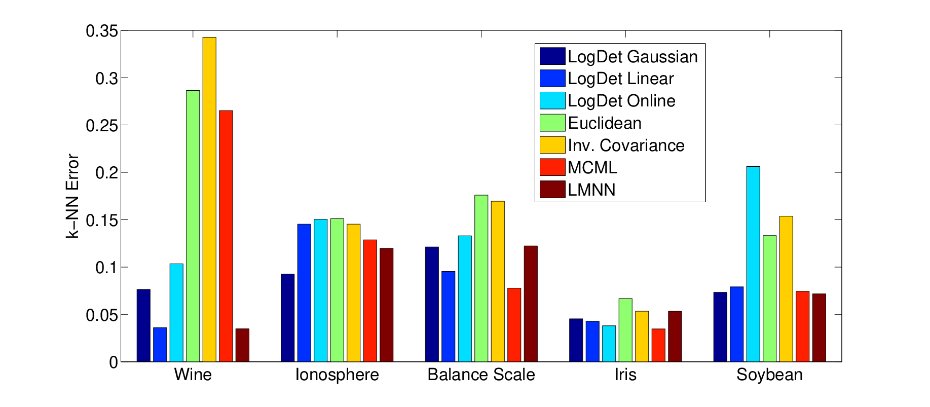
Refer to caption — Figure 1: Results over benchmark UCI data sets. LogDet metric learning was run with in input space (LogDet Linear) as well as in kernel space with a Gaussian kernel (LogDet Gaussian).

First we evaluate our metric learning method on the standard UCI datasets in the low-dimensional (non-kernelized) setting, to directly compare with several existing metric learning methods. In Figure 1, we compare LogDet Linear ( $K_{0}$ equals the linear kernel) and the LogDet Gaussian ( $K_{0}$ equals Gaussian kernel in kernel space) algorithms against existing metric learning methods for $k$ -NN classification. We use the squared Euclidean distance, $d(\bm{x},\bm{y})=(\bm{x}-\bm{y})^{T}(\bm{x}-\bm{y})$ as a baseline method. We also use a Mahalanobis distance parameterized by the inverse of the sample covariance matrix. This method is equivalent to first performing a standard PCA whitening transform over the feature space and then computing distances using the squared Euclidean distance. We compare our method to two recently proposed algorithms: Maximally Collapsing Metric Learning [GR05] (MCML), and metric learning via Large Margin Nearest Neighbor [WBS05] (LMNN). Consistent with existing work such as [GR05], we found the method of [XNJR02] to be very slow and inaccurate, so the latter was not included in our experiments. As seen in Figure 1, LogDet Linear and LogDet Gaussian algorithms obtain somewhat higher accuracy for most of the datasets.

In addition to our evaluations on standard UCI datasets, we also apply our algorithm to the recently proposed problem of nearest neighbor software support for the Clarify system [HRD+07]. The basis of the Clarify system lies in the fact that modern software design promotes modularity and abstraction. When a program terminates abnormally, it is often unclear which component should be responsible for (or is capable of) providing an error report. The system works by monitoring a set of predefined program features (the datasets presented use function counts) during program runtime which are then used by a classifier in the event of abnormal program termination. Nearest neighbor searches are particularly relevant to this problem. Ideally, the neighbors returned should not only have the correct class label, but should also represent those with similar program configurations or program inputs. Such a matching can be a powerful tool to help users diagnose the root cause of their problem. The four datasets we use correspond to the following softwares: Latex (the document compiler, 9 classes), Mpg321 (an mp3 player, 4 classes), Foxpro (a database manager, 4 classes), and Iptables (a Linux kernel application, 5 classes).

Our experiments on the Clarify system, like the UCI data, are over fairly low-dimensional data. It was shown [HRD+07] that high classification accuracy can be obtained by using a relatively small subset of available features. Thus, for each dataset, we use a standard information gain feature selection test to obtain a reduced feature set of size 20. From this, we learn metrics for $k$ -NN classification using the methods developed in this paper. Results are given in Figure 2(b). The LogDet Linear algorithm yields significant gains for the Latex benchmark. Note that for datasets where Euclidean distance performs better than using the inverse covariance metric, the LogDet Linear algorithm that normalizes to the standard Euclidean distance yields higher accuracy than that regularized to the inverse covariance matrix (LogDet-Inverse Covariance). In general, for the Mpg321, Foxpro, and Iptables datasets, learned metrics yield only marginal gains over the baseline Euclidean distance measure.

Figure 2(c) shows the error rate for the Latex datasets with a varying number of features (the feature sets are again chosen using the information gain criteria). We see here that LogDet Linear is surprisingly robust. Euclidean distance, MCML, and LMNN all achieve their best error rates for five dimensions. LogDet Linear, however, attains its lowest error rate of .15 at $d=20$ dimensions.

In Table 1, we see that LogDet Linear generally learns metrics significantly faster than other metric learning algorithms. The implementations for MCML and LMNN were obtained from their respective authors. The timing tests were run on a dual processor 3.2 GHz Intel Xeon processor running Ubuntu Linux. Time given is in seconds and represents the average over 5 runs.

Table 1: Training time (in seconds) for the results presented in Figure 2(b).

Dataset	LogDet Linear	MCML	LMNN
Latex	0.0517	19.8	0.538
Mpg321	0.0808	0.460	0.253
Foxpro	0.0793	0.152	0.189
Iptables	0.149	0.0838	4.19

We also present some semi-supervised clustering results for two of the UCI data sets. Note that both MCML and LMNN are not amenable to optimization subject to pairwise distance constraints. Instead, we compare our method to the semi-supervised clustering algorithm HMRF-KMeans [BBM04]. We use a standard 2-fold cross validation approach for evaluating semi-supervised clustering results. Distances are constrained to be either similar or dissimilar, based on class values, and are drawn only from the training set. The entire dataset is then clustered into $c$ clusters using $k$ -means (where $c$ is the number of classes) and error is computed using only the test set. Table 2 provides results for the baseline $k$ -means error, as well as semi-supervised clustering results with 50 constraints.

Table 2: Unsupervised

k

-means clustering error using the baseline squared Euclidean distance, along with semi-supervised clustering error with 50 constraints.

Dataset	Unsupervised	LogDet Linear	HMRF-KMeans
Ionosphere	0.314	0.113	0.256
Digits-389	0.226	0.175	0.286

6.2 Metric Learning for Object Recognition

Next we evaluate our method over high-dimensional data applied to the object-recognition task using Caltech-101 [Cal04], a common benchmark for this task. The goal is to predict the category of the object in the given image using a $k$ -NN classifier.

We compute distances between images using learning kernels with three different base image kernels: 1) PMK: Grauman and Darrell’s pyramid match kernel [GD05] applied to SIFT features, 2) CORR: the kernel designed by [ZBMM06] applied to geometric blur features , and 3) SUM: the average of four image kernels, namely, PMK [GD05], Spatial PMK [LSP06], Geoblur-1, and Geoblur-2 [BM01]. Note that the underlying dimensionality of these embeddings are typically in the millions of dimensions.

We evaluate the effectiveness of metric/kernel learning on this dataset. We pose a $k$ -NN classification task, and evaluate both the original (SUM, PMK or CORR) and learned kernels. We set $k=1$ for our experiments; this value was chosen arbitrarily. We vary the number of training examples $T$ per class for the database, using the remainder as test examples, and measure accuracy in terms of the mean recognition rate per class, as is standard practice for this dataset.

Figure 3 shows our results relative to several other existing techniques that have been applied to this dataset. Our approach outperforms all existing single-kernel classifier methods when using the learned CORR kernel: we achieve 61.0% accuracy for $T=15$ and 69.6% accuracy for $T=30$ . Our learned PMK achieves 52.2% accuracy for $T=15$ and 62.1% accuracy for $T=30$ . Similarly, our learned SUM kernel achieves $73.7\%$ accuracy for $T=15$ . Figure 4 specifically shows the comparison of the original baseline kernels for NN classification. The plot reveals gains in 1-NN classification accuracy; notably, our learned kernels with simple NN classification also outperform the baseline kernels when used with SVMs [ZBMM06, GD05].

6.3 Metric Learning for Text Classification

Next we present results in the text domain. Our text datasets are created by standard bag-of-words Tf-Idf representations. Words are stemmed using a standard Porter stemmer and common stop words are removed, and the text models are limited to the 5,000 words with the largest document frequency counts. We provide experiments for two data sets: CMU Newsgroups [CMU08], and Classic3 [Cla08]. Classic3 is a relatively small 3 class problem with 3,891 instances. The newsgroup data set is much larger, having 20 different classes from various newsgroup categories and 20,000 instances.

As mentioned earlier, our text experiments use a linear kernel, and we use a set of basis vectors that is constructed from the class labels via the following procedure. Let $c$ be the number of distinct classes and let $k$ be the size of the desired basis. If $k=c$ , then each class mean $r_{i}$ is computed to form the basis $R=[{\bm{r}_{1}}\ldots{\bm{r}_{c}}]$ . If $k<c$ a similar process is used but restricted to a randomly selected subset of $k$ classes. If $k>c$ , instances within each class are clustered into approximately $\frac{k}{c}$ clusters. Each cluster’s mean vector is then computed to form the set of low-rank basis vectors $R$ .

Figure 5 shows classification accuracy across bases of varying sizes for the Classic3 dataset, along with the newsgroup data set. As baseline measures, the standard squared Euclidean distance is shown, along with Latent Semantic Analysis (LSA) [DDL+90], which works by projecting the data via principal components analysis (PCA), and computing distances in this projected space. Comparing our algorithm to the baseline Euclidean measure, we can see that for smaller bases, the accuracy of our algorithm is similar to the Euclidean measure. As the size of the basis increases, our method obtains significantly higher accuracy compared to the baseline Euclidean measure.

7 Conclusions

In this paper, we have considered the general problem of learning a linear transformation of input data and applied it to the problem of learning a metric over high-dimensional data or feature space implicitly. $\phi(\bm{x}_{i})^{T}A\phi(\bm{x}_{j})$ . We first showed that the LogDet divergence is a useful loss for learning a linear transformation (or performing metric learning) in kernel space, as the algorithm can easily be generalized to work in kernel space. We then proposed an algorithm based on Bregman projections to learn a kernel function over the data-points efficiently. We also show that our learned metric can be restricted to a small dimensional basis efficiently, hence scaling our method to large datasets with high-dimensional feature space. Then we considered a larger class of convex loss functions for learning the metric/kernel using a linear transformation of the data; we saw that many loss functions can lead to kernelization, though the resulting optimizations may be more expensive to solve than the simpler LogDet formulation. Finally, we presented some experiments on benchmark data, high-dimensional vision, and text classification problems, demonstrating our method compared to several existing state-of-the-art techniques.

There are several directions of future work. To facilitate even larger data sets than the ones considered in this paper, online learning methods are one promising research direction; in [JKDG08], an online learning algorithm was proposed based on LogDet regularization, and this remains a part of our ongoing efforts. Recently, there has been some interest in learning multiple local metrics over the data; [WS08] considered this problem. We plan to explore this setting with the LogDet divergence, with a focus on scalability to very large data sets.

Acknowledgements

This research was supported by NSF grant CCF-0728879. We would also like to acknowledge Suvrit Sra for various helpful discussions.

References

[AK07] S. Arora and S. Kale. A combinatorial, primal-dual approach to semidefinite programs. In ACM Symposium on Theory of Computing (STOC), pages 227–236. 2007.
[BBM04] S. Basu, M. Bilenko, and R. J. Mooney. A probabilistic framework for semi-supervised clustering. In ACM SIGKDD Int. Conf. on Knowledge Discovery and Data Mining (KDD). 2004.
[BM01] A. C. Berg and J. Malik. Geometric blur for template matching. In IEEE International Conference on Computer Vision and Pattern Recognition (CVPR). 2001.
[Cal04] Caltech-101 Data Set. Public Dataset, 2004. [link].
[CHL05] S. Chopra, R. Hadsell, and Y. LeCun. Learning a similarity metric discriminatively, with application to face verification. In IEEE International Conference on Computer Vision and Pattern Recognition (CVPR). 2005.
[CKTK08] R. Chatpatanasiri, T. Korsrilabutr, P. Tangchanachaianan, and B. Kijsirikul. On kernelization of supervised Mahalanobis distance learners. ArXiv, 2008. http://arxiv.org/pdf/0804.1441.
[Cla08] Classic3 Data Set. ftp.cs.cornell.edu/pub/smart, 2008.
[CMU08] CMU 20-Newsgroups Data Set. http://www.cs.cmu.edu/afs/cs.cmu.edu/project/theo-20/www/data/news20.html, 2008.
[DD08] J. V. Davis and I. S. Dhillon. Structured metric learning for high dimensional problems. In ACM SIGKDD Int. Conf. on Knowledge Discovery and Data Mining (KDD), pages 195–203. 2008.
[DDL⁺90] S. C. Deerwester, S. T. Dumais, T. K. Landauer, G. W. Furnas, and R. A. Harshman. Indexing by latent semantic analysis. Journal of the American Society of Information Science, 41(6):391–407, 1990.
[DKJ⁺07] J. Davis, B. Kulis, P. Jain, S. Sra, and I. Dhillon. Information-theoretic metric learning. In Int. Conf. on Machine Learning (ICML). 2007.
[Fle91] R. Fletcher. A new variational result for quasi-newton formulae. SIAM Journal on Optimization, 1(1), 1991.
[GD05] K. Grauman and T. Darrell. The Pyramid Match Kernel: Discriminative Classification with Sets of Image Features. In International Conference on Computer Vision (ICCV). 2005.
[GLS88] M. Groschel, L. Lovasz, and A. Schrijver. Geometric Algorithms and Combinatorial Optimization. Springer-Verlag, 1988.
[GR05] A. Globerson and S. Roweis. Metric learning by collapsing classes. In Adv. in Neural Inf. Proc. Sys. (NIPS). 2005.
[GRHS04] J. Goldberger, S. Roweis, G. Hinton, and R. Salakhutdinov. Neighbourhood component analysis. In Adv. in Neural Inf. Proc. Sys. (NIPS). 2004.
[Hig08] N. J. Higham. Functions of Matrices: Theory and Computation. SIAM, 2008.
[HRD⁺07] J. Ha, C. Rossbach, J. Davis, I. Roy, D. Chen, H. Ramadan, and E. Witchel. Improved error reporting for software that uses black box components. In Programming Language Design and Implementation (PLDI). 2007.
[HT96] T. Hastie and R. Tibshirani. Discriminant adaptive nearest neighbor classification. IEEE Transactions on Pattern Analysis and Machine Intelligence, 18:607–616, 1996.
[JKDG08] P. Jain, B. Kulis, I. S. Dhillon, and K. Grauman. Online metric learning and fast similarity search. In Adv. in Neural Inf. Proc. Sys. (NIPS), pages 761–768. 2008.
[JS61] W. James and C. Stein. Estimation with quadratic loss. In Fourth Berkeley Symposium on Mathematical Statistics and Probability, volume 1, pages 361–379. Univ. of California Press, 1961.
[KSD06] B. Kulis, M. Sustik, and I. S. Dhillon. Learning low-rank kernel matrices. In Int. Conf. on Machine Learning (ICML). 2006.
[KSD08] B. Kulis, M. Sustik, and I. Dhillon. Low-rank kernel learning with Bregman matrix divergences. Journal of Machine Learning Research, 2008.
[KSD09] B. Kulis, S. Sra, and I. S. Dhillon. Convex perturbations for scalable semidefinite programming. In International Conference on Artificial Intelligence and Statistics (AISTATS). 2009.
[KT03] J. Kwok and I. Tsang. Learning with idealized kernels. In Int. Conf. on Machine Learning (ICML). 2003.
[LCB⁺04] G. R. G. Lanckriet, N. Cristianini, P. Bartlett, L. El Ghaoui, and M. I. Jordan. Learning the kernel matrix with semidefinite programming. In Journal of Machine Learning Research. 2004.
[Leb06] G. Lebanon. Metric learning for text documents. IEEE Transactions on Pattern Analysis and Machine Intelligence, 28(4):497–508, 2006.
[LSP06] S. Lazebnik, C. Schmid, and J. Ponce. Beyond bags of features: Spatial pyramid matching for recognizing natural scene categories. In IEEE International Conference on Computer Vision and Pattern Recognition (CVPR), pages 2169–2178. 2006.
[NC00] M.A. Nielsen and I.L. Chuang. Quantum Computation and Quantum Information. Cambridge University Press, 2000.
[OSW03] C. S. Ong, A. J. Smola, and R. C. Williamson. Hyperkernels. In Adv. in Neural Inf. Proc. Sys. (NIPS). 2003.
[SHWP02] N. Shental, T. Hertz, D. Weinshall, and M. Pavel. Adjustment learning and relevant component analysis. In European Conference on Computer Vision (ECCV). Copenhagen, DK, 2002.
[SJ03] M. Schutz and T. Joachims. Learning a distance metric from relative comparisons. In Adv. in Neural Inf. Proc. Sys. (NIPS). 2003.
[SSSN04] S. Shalev-Shwartz, Y. Singer, and A. Y. Ng. Online and batch learning of pseudo-metrics. In Int. Conf. on Machine Learning (ICML). 2004.
[TK06] I. W. Tsang and J. T. Kwok. Efficient hyperkernel learning using second-order cone programming. IEEE Transactions on Neural Networks, 17(1):48–58, 2006.
[TRW05] K. Tsuda, G. Rátsch, and M. Warmuth. Matrix exponentiated gradient updates for online learning and Bregman projection. Journal of Machine Learning Research, 6:995–1018, 2005.
[WBS05] K. Q. Weinberger, J. Blitzer, and L. K. Saul. Distance metric learning for large margin nearest neighbor classification. In Adv. in Neural Inf. Proc. Sys. (NIPS). 2005.
[WK08] M. K. Warmuth and D. Kuzmin. Randomized online PCA algorithms with regret bounds that are logarithmic in the dimension. Journal of Machine Learning Research, 9:2287–2320, 2008.
[WS08] K. Q. Weinberger and L. K. Saul. Fast solvers and efficient implementations for distance metric learning. In Int. Conf. on Machine Learning (ICML). 2008.
[XNJR02] E. P. Xing, A. Y. Ng, M. I. Jordan, and S. Russell. Distance metric learning with application to clustering with side-information. In Adv. in Neural Inf. Proc. Sys. (NIPS), volume 14. 2002.
[ZBMM06] H. Zhang, A. Berg, M. Maire, and J. Malik. SVM-KNN: Discriminative Nearest Neighbor Classification for Visual Category Recognition. In IEEE International Conference on Computer Vision and Pattern Recognition (CVPR). 2006.

	$\displaystyle W^{*}$	$\displaystyle=\sum_{j=1}^{n}\lambda_{i}^{}\bm{u}_{j}^{}\bm{u}_{j}^{T}+\eta\sum_{j=n+1}^{d}\bm{u}_{j}^{}\bm{u}_{j}^{*T},$
		$\displaystyle=\sum_{j=1}^{n}(\lambda_{i}^{}-\eta)\bm{u}_{j}^{}\bm{u}_{j}^{T}+\eta\sum_{j=1}^{d}\bm{u}_{j}^{}\bm{u}_{j}^{*T},$
		$\displaystyle=\sum_{j=1}^{n}X((\lambda_{j}^{}-\eta)\bm{\alpha}_{j}^{}\bm{\alpha}_{j}^{*T})X^{T}+\eta I^{d},$
		$\displaystyle=XS^{*}X^{T}+\eta I^{d},$