Which graphical models are difficult to learn?

Given a graph $G=(V=[p],E)$, and a positive parameter $\theta>0$ the ferromagnetic Ising model on $G$ is the pairwise Markov random field

over binary variables $\underline{x}=(x_{1},x_{2},\dots,x_{p})$. Apart from being one of the most studied models in statistical mechanics, the Ising model is a prototypical undirected graphical model, with applications in computer vision, clustering and spatial statistics. Its obvious generalization to edge-dependent parameters $\theta_{ij}$, $(i,j)\in E$ is of interest as well, and will be introduced in Section 1.2.2. (Let us stress that we follow the statistical mechanics convention of calling (1) an Ising model for any graph $G$.)

In this paper we study the following structural learning problem: Given $n$ i.i.d. samples $\underline{x}^{(1)}$, $\underline{x}^{(2)}$,…, $\underline{x}^{(n)}$ with distribution $\mu_{G,\theta}(\,\cdot\,)$, reconstruct the graph $G$. For the sake of simplicity, we assume that the parameter $\theta$ is known, and that $G$ has no double edges (it is a ‘simple’ graph).

The graph learning problem is solvable with unbounded sample complexity, and computational resources [1]. The question we address is: for which classes of graphs and values of the parameter $\theta$ is the problem solvable under appropriate complexity constraints? More precisely, given an algorithm ${\sf Alg}$, a graph $G$, a value $\theta$ of the model parameter, and a small $\delta>0$, the sample complexity is defined as

where ${\mathbb{P}}_{n,G,\theta}$ denotes probability with respect to $n$ i.i.d. samples with distribution $\mu_{G,\theta}$. Further, we let $\chi_{{\sf Alg}}(G,\theta)$ denote the number of operations of the algorithm ${\sf Alg}$, when run on $n_{{\sf Alg}}(G,\theta)$ samples.¹¹ 1 For the algorithms analyzed in this paper, the behavior of $n_{{\sf Alg}}$ and $\chi_{{\sf Alg}}$ does not change significantly if we require only ‘approximate’ reconstruction (e.g. in graph distance).

The general problem is therefore to characterize the functions $n_{{\sf Alg}}(G,\theta)$ and $\chi_{{\sf Alg}}(G,\theta)$, in particular for an optimal choice of the algorithm. General bounds on $n_{{\sf Alg}}(G,\theta)$ have been given in [2, 3], under the assumption of unbounded computational resources. A general charactrization of how well low complexity algorithms can perform is therefore lacking. Although we cannot prove such a general characterization, in this paper we estimate $n_{{\sf Alg}}$ and $\chi_{{\sf Alg}}$ for a number of graph models, as a function of $\theta$, and unveil a fascinating universal pattern: when the model (1) develops long range correlations, low-complexity algorithms fail. Under the Ising model, the variables $\{x_{i}\}_{i\in V}$ become strongly correlated for $\theta$ large. For a large class of graphs with degree bounded by $\Delta$, this phenomenon corresponds to a phase transition beyond some critical value of $\theta$ uniformly bounded in $p$, with typically $\theta_{\rm crit}\leq{\rm const.}/\Delta$. In the examples discussed below, the failure of low-complexity algorithms appears to be related to this phase transition (although it does not coincide with it).

In order to explore the practical relevance of the above results, we carried out extensive numerical simulations using the regularized logistic regression algorithm ${\sf Rlr}(\lambda)$. Among other learning algorithms, ${\sf Rlr}(\lambda)$ strikes a good balance of complexity and performance. Samples from the Ising model (1) where generated using Gibbs sampling (a.k.a. Glauber dynamics). Mixing time can be very large for $\theta\geq\theta_{\rm crit}$, and was estimated using the time required for the overall bias to change sign (this is a quite conservative estimate at low temperature). Generating the samples $\{\underline{x}^{(\ell)}\}$ was indeed the bulk of our computational effort and took about $50$ days CPU time on Pentium Dual Core processors (we show here only part of these data). Notice that ${\sf Rlr}(\lambda)$ had been tested in [7] only on tree graphs $G$, or in the weakly coupled regime $\theta<\theta_{\rm crit}$. In these cases sampling from the Ising model is easy, but structural learning is also intrinsically easier.

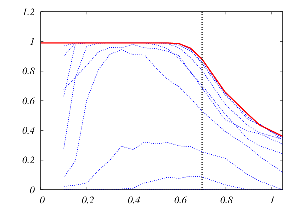
Figure reports the success probability of ${\sf Rlr}(\lambda)$ when applied to random subgraphs of a $7\times 7$ two-dimensional grid. Each such graphs was obtained by removing each edge independently with probability $\rho=0.3$. Success probability was estimated by applying ${\sf Rlr}(\lambda)$ to each vertex of $8$ graphs (thus averaging over $392$ runs of ${\sf Rlr}(\lambda)$), using $n=4500$ samples. We scaled the regularization parameter as $\lambda=2\lambda_{0}\theta(\log p/n)^{1/2}$ (this choice is motivated by the algorithm analysis and is empirically the most satisfactory), and searched over $\lambda_{0}$.

The data clearly illustrate the phenomenon discussed. Despite the large number of samples $n\gg\log p$, when $\theta$ crosses a threshold, the algorithm starts performing poorly irrespective of $\lambda$. Intriguingly, this threshold is not far from the critical point of the Ising model on a randomly diluted grid $\theta_{\rm crit}(\rho=0.3)\approx 0.7$ [15, 16].

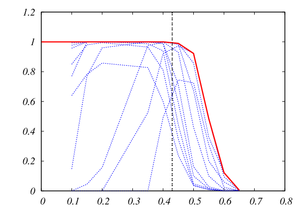
Figure 2 presents similar data when $G$ is a uniformly random graph of degree $\Delta=4$, over $p=50$ vertices. The evolution of the success probability with $n$ clearly shows a dichotomy. When $\theta$ is below a threshold, a small number of samples is sufficient to reconstruct $G$ with high probability. Above the threshold even $n=10^{4}$ samples are to few. In this case we can predict the threshold analytically, cf. Lemma 3.3 below, and get $\theta_{\rm thr}(\Delta=4)\approx 0.4203$, which compares favorably with the data.

In order to prove Theorem 1.6, we need a few auxiliary results. It is convenient to introduce some notations. If $M$ is a matrix and $R,P$ are index sets then $M_{R\;P}$ denotes the submatrix with row indices in $R$ and column indices in $P$. As above, we let $r$ be the vertex whose neighborhood we are trying to reconstruct and define $S={\partial r}$, $S^{c}=V\setminus{{\partial r}\cup r}$. Since the cost function $L(\underline{\theta};\{x^{(\ell)}\})+\lambda||\underline{\theta}||_{1}$ only depend on $\underline{\theta}$ through its components $\underline{\theta}_{r,\cdot}=\{\theta_{rj}\}$, we will hereafter neglect all the other parameters and write $\underline{\theta}$ as a shorthand of $\underline{\theta}_{r,\cdot}$.

Let $\hat{z}^{*}$ be a subgradient of $||\underline{\theta}||_{1}$ evaluated at the true parameters values, $\underline{\theta}^{*}=\{\theta_{rj}:\theta_{ij}=0,\;\forall j\notin{\partial r},\theta_{rj}=\theta,\;\forall j\in{\partial r}\}$. Let $\hat{\underline{\theta}}^{n}$ be the parameter estimate returned by ${\sf Rlr}(\lambda)$ when the number of samples is $n$. Note that, since we assumed $\underline{\theta}^{*}\geq 0$, $\hat{z}^{*}_{S}=\mathbbm{1}$. Define $Q^{n}(\underline{\theta},;\{\underline{x}^{(\ell)}\})$ to be the Hessian of $L(\underline{\theta};\{x^{(\ell)}\})$ and $Q(\underline{\theta})=\lim_{n\rightarrow\infty}Q^{n}(\underline{\theta},;\{\underline{x}^{(\ell)}\})$. By the law of large numbers $Q(\underline{\theta})$ is the Hessian of ${\mathbb{E}}_{G,\underline{\theta}}\log{\mathbb{P}}_{G,\underline{\theta}}(X_{r}|X_{\backslash r})$ where ${\mathbb{E}}_{G,\underline{\theta}}$ is the expectation with respect to (8) and $\underline{X}$ is a random variable distributed according to (8). We will denote the maximum and minimum eigenvalue of a symmetric matrix $M$ by $\sigma_{\rm max}(M)$ and $\sigma_{\rm min}(M)$ respectively.

We will omit arguments whenever clear from the context. Any quantity evaluated at the true parameter values will be represented with a ^∗, e.g. $Q^{*}=Q(\theta^{*})$. Quantities under a $\wedge$ depend on $n$. Throughout this section $G$ is a graph of maximum degree $\Delta$.

References

- [1] P. Abbeel, D. Koller and A. Ng, “Learning factor graphs in polynomial time and sample complexity”. Journal of Machine Learning Research., 2006, Vol. 7, 1743–1788.
- [2] M. Wainwright, “Information-theoretic limits on sparsity recovery in the high-dimensional and noisy setting”, arXiv:math/0702301v2 [math.ST], 2007.
- [3] N. Santhanam, M. Wainwright, “Information-theoretic limits of selecting binary graphical models in high dimensions”, arXiv:0905.2639v1 [cs.IT], 2009.
- [4] G. Bresler, E. Mossel and A. Sly, “Reconstruction of Markov Random Fields from Samples: Some Observations and Algorithms”,Proceedings of the 11th international workshop, APPROX 2008, and 12th international workshop RANDOM 2008, 2008 ,343–356.
- [5] Csisz�ar and Z. Talata, “Consistent estimation of the basic neighborhood structure of Markov random fields”, The Annals of Statistics, 2006, 34, Vol. 1, 123-�145.
- [6] N. Friedman, I. Nachman, and D. Peer, “Learning Bayesian network structure from massive datasets: The �sparse candidate� algorithm”. In UAI, 1999.
- [7] P. Ravikumar, M. Wainwright and J. Lafferty, “High-Dimensional Ising Model Selection Using l1-Regularized Logistic Regression”, arXiv:0804.4202v1 [math.ST], 2008.
- [8] M.Wainwright, P. Ravikumar, and J. Lafferty, “Inferring graphical model structure using l1-regularized pseudolikelihood“, In NIPS, 2006.
- [9] H. Höfling and R. Tibshirani, “Estimation of Sparse Binary Pairwise Markov Networks using Pseudo-likelihoods” , Journal of Machine Learning Research, 2009, Vol. 10, 883–906.
- [10] O.Banerjee, L. El Ghaoui and A. d’Aspremont, “Model Selection Through Sparse Maximum Likelihood Estimation for Multivariate Gaussian or Binary Data”, Journal of Machine Learning Research, March 2008, Vol. 9, 485–516.
- [11] M. Yuan and Y. Lin, “Model Selection and Estimation in Regression with Grouped Variables”, J. Royal. Statist. Soc B, 2006, 68, Vol. 19,49–67.
- [12] N. Meinshausen and P. Büuhlmann, “High dimensional graphs and variable selection with the lasso”, Annals of Statistics, 2006, 34, Vol. 3.
- [13] R. Tibshirani, “Regression shrinkage and selection via the lasso”, Journal of the Royal Statistical Society, Series B, 1994, Vol. 58, 267–288.
- [14] P. Zhao, B. Yu, “On model selection consistency of Lasso”, Journal of Machine. Learning Research 7, 2541–2563, 2006.
- [15] D. Zobin, ”Critical behavior of the bond-dilute two-dimensional Ising model“, Phys. Rev., 1978 ,5, Vol. 18, 2387 – 2390.
- [16] M. Fisher, ”Critical Temperatures of Anisotropic Ising Lattices. II. General Upper Bounds”, Phys. Rev. 162 ,Oct. 1967, Vol. 2, 480–485.
- [17] A. Dembo and A. Montanari, “Ising Models on Locally Tree Like Graphs”, Ann. Appl. Prob. (2008), to appear, arXiv:0804.4726v2 [math.PR]