Decoherence in an Interacting Quantum Field Theory:
The Vacuum Case
Abstract
We apply the decoherence formalism to an interacting scalar field theory. In the spirit of the decoherence literature, we consider a “system field” and an “environment field” that interact via a cubic coupling. We solve for the propagator of the system field, where we include the self-energy corrections due to the interaction with the environment field. In this paper, we consider an environment in the vacuum state (). We show that neglecting inaccessible non-Gaussian correlators increases the entropy of the system as perceived by the observer. Moreover, we consider the effect of a changing mass of the system field in the adiabatic regime, and we find that at late times no additional entropy has been generated.
pacs
03.65.Yz, 03.70.+k, 03.67.-a, 98.80.-kI Introduction
I.1 Outline
We aim to apply the decoherence formalism to an interacting quantum field theoretical model. The main idea in the framework of decoherence ([1, 2, 3, 4], for reviews see [5, 6, 7, 8, 9]) is that a macroscopic system cannot be separated from its environment. The conventional strategy is to assume the existence of a distinct system, environment and observer. If the observer and the environment are weakly coupled, we are allowed to integrate the environment out to study its average effect on the system perceived by the observer. Alternatively one could say that the environmental degrees of freedom are inaccessible to the observer. This averaging process is an intrinsically non-unitary operation, which consequently gives rise to an increase in entropy of the system. A quantum system with a large entropy, in turn, corresponds to an effectively classical system.
It is however difficult to realistically apply the decoherence machinery to quantum field theory: this requires in general involved out-of-equilibrium, finite temperature, interacting quantum field theoretical computations. It is of course widely appreciated that entropy can be generated as a result of an incomplete knowledge of a system. We thus need to keep in mind what quantities are actually measured in quantum field theory: all information in a system that can in principle be observed by a “perfect observer” is contained in the -point correlators of the system. However, realistic observers are not capable of measuring irreducible -point functions of arbitrary order as they are limited by the sensitivity of their apparatus. Therefore, it is important to realise that inaccessible higher order correlators, from the observer’s perspective, yield an increase in entropy of the system. We thus propose the following viewpoint when applying the decoherence program to quantum field theory11 1 Older work can already be interpreted in a similar spirit [10, 11]. Here, we propose it as a strict procedure [12, 13] of how to study entropy generation in the 2PI formalism, also see [14]. Recently, during the last stages of writing this paper, we found an interesting article by Giraud and Serreau [15] addressing the question of entropy production in an interacting field theory from a similar perspective.:
Neglecting observationally inaccessible correlators will give rise to an increase in entropy of the system as perceived by the observer.
As an example, consider some interacting quantum field theory where information is stored in either two-point or Gaussian correlators or in higher order, non-Gaussian correlators. The latter are generated generically in any interacting field theory. If we assume that the information stored in these non-Gaussian correlators is barely accessible in experiments, then neglecting this information will give rise to an increase in the entropy. From the Gaussian correlators, we can fix the entropy uniquely [16, 14]. As before, a quantum system with a considerable amount of entropy corresponds to a classical system22 2 Our definition of classicality differs from the approach used in some of the literature, where for example coherent states with large occupation numbers are also considered to have many classical properties, even though these states have vanishing entropy.. We emphasise that this definition can be improved if e.g. three- or four-point correlators are accessible through experiments such that knowledge of these correlators is included in the definition of the entropy [14]. It is important to stress that this procedure does not require a non-unitary process of tracing out environmental degrees of freedom.
In order to apply these rather abstract ideas to a scalar field toy model, let us outline our paper. We will consider the following interacting scalar field theory:
| (1) |
where:
| (2a) | |||||
| (2b) | |||||
| (2c) | |||||
where is the -dimensional Minkowski metric. Here, will play the role of the system, interacting with an environment , where we assume that such that the environment is in thermal equilibrium at temperature . In this paper, we study an environment of temperature , i.e.: an environment in its vacuum state and we postpone the finite temperature corrections to a future publication. We assume that , which can be realised by suitably renormalising the tadpoles.
Another application of our calculation is baryogenesis in an early Universe setting where the system is driven out-of-equilibrium by a changing mass term generated by a time dependent Higgs-like scalar field during a symmetry breaking. For electroweak baryogenesis, we can neglect the Universe’s expansion during the phase transition and our assumption to work in Minkowski spacetime is well justified.
As we study out-of-equilibrium quantum field theory, we work in the Schwinger-Keldysh formalism. The 2PI (two particle irreducible) effective action then captures the effect of perturbative loop corrections to the various propagators and . Of course we will discuss these equations of motion in greater detail in the main text, but when we omit all indices and arguments, they have the following structure:
| (3a) | |||||
| (3b) | |||||
where and are the corresponding self-masses. These two equations are non-Gaussian due to the coupling of the two fields with coupling constant . Multiplying equation (3a) by and equation (3b) by and integrating, one gets the following Schwinger-Dyson equations:
![[Uncaptioned image]](0910.5733v3/Feynmandiagrams3.png) |
|||||
![[Uncaptioned image]](0910.5733v3/Feynmandiagrams7.png)
![[Uncaptioned image]](0910.5733v3/Feynmandiagrams8.png) +
+The dressed -propagators (double solid lines) can be written as the sum of the tree level propagators (solid lines) and the self-mass corrections due to interaction with the dressed -field (double dashed lines), and vice versa for the environment field.
Let us at this point explicitly state the two main assumptions of our work. Firstly, we assume that our observer is only sensitive to Gaussian correlation functions. This implies that we use only these correlators to calculate the entropy [14]. Secondly, we neglect the backreaction from the system field on the environment field, i.e.: we assume that we can neglect the self-mass corrections due to the -field in equation (4). This assumption thus implies that the environment remains at temperature . In particular, the self-mass corrections to the system propagators in equation (4) are now given by:
![[Uncaptioned image]](0910.5733v3/Feynmandiagrams4.png)
![[Uncaptioned image]](0910.5733v3/Feynmandiagrams5.png)
|
(5) |
The first diagram contains the leading order self-mass correction, at order , where . It effectively is a Gaussian correction to the -propagators as it acts just like a known source to . Note that in equation (5) we dropped a diagram at order since it is irrelevant for the argument presented below.
Looking at equation (5) we see that these assumptions are well justified by perturbative arguments provided there are no secular effects: the backreaction of the system field on the environment field and the first intrinsically non-Gaussian correction occurs only at order , which can be appreciated by examining the second Feynman diagram on the righthand side of equation (5). The 3-point function of the system, an intrinsically non-Gaussian correlator, is at one-loop level also perturbatively suppressed at order .
Finally, let us just mention that the concept of the pointer basis is frequently discussed in the decoherence literature. The pointer basis of our theory in the highly squeezed limit is the field amplitude basis [14], occurring for example in cosmological perturbation theory. Intuitively, this can be appreciated as follows: the Hamiltonian of a squeezed state is dominated by the potential term. A system in interaction with an environment at temperature minimises its free energy . The system will realise this by increasing its entropy , mainly due to increasing the spread in momentum since that hardly affects the Hamiltonian, whereas it does significantly affect the entropy. In other words: the field amplitude basis is robust under the process of decoherence, qualifying it as a proper pointer basis. Note that is a pointer basis only in the statistical sense, such that there is a well defined probability distribution function from which a measurement is drawn.
Having discussed the setup of our theory, the assumptions used and their justification, let us direct our attention to discussing potential applications. Our results are relevant for several research areas: the study of decoherence of cosmological perturbations, of out-of-equilibrium quantum field theory and of baryogenesis.
I.2 Decoherence of Cosmological Perturbations
Although applications of the framework of decoherence are mainly directed towards experimental efforts (for example related to the increasingly relevant field of quantum computing), it also concerns quantum field theory (see e.g.: [17]). Research efforts are primarily focused on addressing the fundamental question of the decoherence of cosmological perturbations, see e.g.: [18, 19, 20, 23, 22, 21, 24, 25, 26, 27, 28, 31, 30, 29, 32, 33, 35, 34, 16, 36]. One of the most important consequences of the inflationary paradigm is that it provides us with a causal explanation of how initial density inhomogeneities can be laid out on super Hubble scales that seed the large scale structure we observe in the Universe today in for example clusters of galaxies. The decoherence formalism applied to cosmological perturbations aims at describing the transition between the quantum nature of the initial density inhomogeneities as a consequence of inflation and the classical stochastic behaviour as assumed by large scale structure theory.
In the literature, specific models for example assume that during inflation the UV (or sub-Hubble) modes of a field, once integrated out, decohere the IR (or super-Hubble) modes because the former modes are inaccessible observationally ([37, 38, 39], however also see [40]). A similar split of UV and IR modes has been made in the context of stochastic inflation, see e.g.: [41, 42, 43, 44, 45, 46]. In [47] vacuum fluctuations decohere the mean field, turning it into a classical stochastic field. In [16] it is argued that self-mass corrections to the equation of motion for the statistical propagator can be rewritten in terms of a stochastic noise term that in turn decoheres the system. In [31] it was shown that isocurvature modes decohere the adiabatic mode.
I.3 Non-equilibrium Quantum Field Theory
In recent years, the study of non-equilibrium quantum field theory has become more and more tractable (for review articles see: [48, 49]). A central ingredient in performing these studies is the two particle irreducible action, from which quantum corrections to propagators can be investigated. Out-of-equilibrium -theory has extensively been studied in for example [52, 50, 53, 54, 55, 56, 57, 58, 51]. The dynamics of non-equilibrium fermions has been addressed in e.g.: [59].
An interesting study has been performed in [60], where one also studies, under certain assumptions, the dynamics of a system field that interacts via a cubic coupling with a thermal bath, which we also consider. Their thermal bath consists of two scalar fields with different masses. Very recently, another interesting calculation for self-interaction has been performed in [15] where one calculates a decoherence parameter and thermalisation of an initial pure state.
Calzetta and Hu consider in [61, 62] also an out-of-equilibrium theory. What we would refer to as “Gaussian von Neumann entropy” is referred to as “correlation entropy” in [62]. They prove an -theorem for a quantum mechanical model.
Renormalising the Kadanoff-Baym equations is a subtle business. In -theory it has been examined in different contexts in [63, 64, 65, 66, 67, 68, 69, 70]. We will also come to address the question of renormalising our cubically interacting field theory. Our main finding is that the structure of the renormalised equations of motion differs from the unrenormalised equations, which has in general to our knowledge not previously been considered in the literature.
Furthermore, imposing initial conditions at some finite time results in additional infinities that have to be renormalised separately according to the authors of [71, 72, 73, 74]. Another interesting study has been performed by [75] in which the renormalised Kadanoff-Baym equations, again in , are numerically integrated by imposing non-Gaussian initial conditions. We differ in our approach as we consider the memory effects from the interacting theory at times before . We can then impose appropriate Gaussian initial conditions at without encountering initial time divergences.
I.4 Baryogenesis
This work is in part inspired by fundamental questions concerning the problem of entropy in field theory, and in part by electroweak scale baryogenesis. The problem is to calculate axial vector currents generated by a CP violating advancing phase interface of a true vacuum bubble at the electroweak phase transition. These currents then feed in hot sphalerons, thus biasing baryon production. The axial currents are difficult to calculate reliably, since a controlled calculation would include non-equilibrium dynamics in a finite temperature plasma in the presence of a non-adiabatically changing mass parameter. In this paper we neither include a plasma at finite temperature (this will be done in a future companion paper), nor do we consider scattering of fermions on a non-adiabatically changing phase interface. Yet there are important similarities between the problem we address here and baryogenesis: our interacting scalar field model (2) mimics the Yukawa part of the lagrangian of the standard model, whereby one scalar field plays the role of the Higgs field, while the other is a heavy fermion (top quark or a chargino of a supersymmetric theory). The role of the axial current is taken by the entropy which are both sensitive to quantum coherence and the phase interface is a time dependent mass parameter . The importance of quantum coherence in baryogenesis is also treated in [76, 77, 78], where a coherent mixture of fermions has been used to generate baryons in grand unified theories during preheating after inflation. However, the authors of [76, 77, 78] treat the interactions phenomenologically in the relaxation time approximation.
Quantum mechanical scattering on bubble walls in a thermal bath may become the dominant mechanism for baryon production when the walls are thin, and has been addressed in several papers in the mid 1990s [79, 80, 81, 82, 83, 84] mostly in the context of baryogenesis within the standard model. Currently, the consensus is that so far no satisfactory solution to the problem has been found. Recently Herranen, Kainulainen and Rahkila [85, 86, 87] have reinvigorated interest in the problem, which has gained on timeliness by the upcoming LHC experiments. Their approach is based on the observation that the constraint equations for fermions and scalars admit a third particle shell at a vanishing energy, . The authors show that this third shell can be used to correctly reproduce the Klein paradox both for fermions and bosons in a step potential, and hope that their intrinsically off-shell formulation can be used to include interactions in a field theoretical settings, for which off-shell physics is essential. The authors have studied both fermionic [85, 86] and bosonic [87] quantum mechanical reflection in the presence of scatterings. However, not all scatterings implied by the Kadanoff-Baym equations are taken into account. One important motivation for the present paper is to work within a set of approximations where all relevant terms in the Kadanoff-Baym equations are kept.
II Entropy and Propagators
II.1 The Statistical Propagator and Entropy
There is a connection between the statistical propagator and the Gaussian entropy of a system ([14], also see: [10, 16]). In quantum field theory, one can calculate many propagators, with different properties associated with each, but not all of them are independent. In this work, we will be primarily interested in solving for the statistical propagator of the system. Let us mention that the information contained in the statistical propagator is also encoded in the two Wightman functions. Generically, in the presence of quantum fluctuations, one needs complete knowledge of the causal propagator in order to solve for the statistical propagator. In the simple free theory example we consider in appendix A, we can directly solve for the statistical propagator however and no prior knowledge of the causal propagator is required.
The statistical propagator describes how states are populated and is in the Heisenberg picture defined by:
| (6) |
given some density matrix operator . The causal propagator roughly describes the number of accessible states and is given by the commutator of the two fields:
| (7) |
In spatially homogeneous backgrounds, we can Fourier transform e.g. the statistical propagator as follows:
| (8) |
which in the case we will consider in this paper only depends on . It is only the statistical propagator and its various time derivatives that determine the entropy. In short, the entropy is fixed by the area in phase space the state of the system occupies and is given by:
| (9) |
Throughout the paper, and in particular in this equation we set . We also set . The entropy per mode then follows as:
| (10) |
Finally, it is interesting to note that the phase space area can be related to an effective phase space particle number density per mode or the statistical particle number density per mode as:
| (11) |
In appendix A we illustrate our ideas by studying a non-trivial exact case: quantum scattering due to a changing mass in the free case, i.e.: the interaction coefficients and in equation (2c) are switched off. For a free scalar field with a smoothly changing mass term, we show that and hence no entropy has been generated by the mass change. Secondly, we point out that the reader should not confuse the statistical particle number density in equation (11) with the parameter characterising non-adiabaticity of the mass change in equation (129b), which in the literature is often referred to as a particle number as well [88]. This parameter is non-zero, and possibly large, simply because the asymptotic in and out vacua differ.
II.2 Propagators in the Schwinger-Keldysh Formalism
The material included in this subsection may well be familiar to the experienced reader, but we include it nevertheless for pedagogical reasons and in order to clearly establish our notation. Let us consider the expectation value of an operator in the Heisenberg picture, given a density matrix operator :
| (12) |
where denotes an initial time, and denote the anti-time ordering and time ordering operations, respectively, and denotes the Hamiltonian. If in the Scrödinger picture depends explicitly on time, we should replace by .
The Schwinger-Keldysh formalism, or closed time path (CTP) formalism, or in-in formalism, is based on the original papers by Schwinger [89] and Keldysh [90] and particularly useful for non-equilibrium quantum field theory (also see: [91, 92, 93, 94, 95]). According to the CTP formalism, the expectation value above can be calculated from the in-in generating functional in the path integral formulation:
| (13) | |||
where the Lagrangian is given in equation (1). We can use the well-known Schwinger-Keldysh contour depicted in figures 2 and 2.


It runs from up to , where both times can in principle be extended to negative and positive infinity, respectively (as depicted in figure 2). As we will come to discuss, the two paths are not equivalent in an interacting quantum field theory, where memory effects play an important role. In this paper, we will extend to negative infinity at some point, but let us for the moment keep it finite. Clearly, these contours are closely related to the two evolution operators in equation (12). The fields and and their corresponding sources and split up on the upper (+) and lower (-) parts of the contour, where necessarily the conditions and apply. These conditions are indeed enforced by the two functional -distributions. The first functional integrals in (13) are over the initial configuration space at , where the system is specified by the density operator (density matrix) . The path integrals in (13) run over the Schwinger-Keldysh contour in figure 2 or 2.
Expectation values of -point functions are obtained by varying the generating functional (13) as follows:
provided that and for all , and where . We can now define the following propagators:
| (14a) | |||||
| (14b) | |||||
| (14c) | |||||
| (14d) | |||||
We define the various propagators for the -field analogously. In the absence of a condensate for all mixed two point functions, such as:
| (15) |
vanish by virtue of the interaction term (2c). In equation (14), denotes the Feynman or time ordered propagator and represents the anti-time ordered propagator. The two Wightman functions are given by and . From equation (1) we infer that the free Feynman propagator obeys:
| (16) |
where and where the same identity holds for . In the presence of interactions the equation of motion for the Feynman propagator becomes much more involved and we will discus it shortly. One can easily show that at tree level the Wightman functions obey the homogeneous equation:
| (17) |
Identical relations hold for the free -propagators. The four propagators defined above are not independent. The Wightman functions for example constitute the time ordered and anti-time ordered propagators:
| (18a) | |||||
| (18b) | |||||
| where , , and where this identity holds for the -propagators as well. Appreciate that: | |||||
| (18c) | |||||
| (18d) | |||||
are exact identities and they are also satisfied by the -propagators. We write the four Green’s functions in the Keldysh propagator matrix form:
| (19) |
which at tree level obeys,
| (20) |
where is the third Pauli matrix, which we can also write as:
| (21) |
where .
Let us define some more Green’s functions. In subsection II.1 we already defined the causal and statistical propagator, but let us for completeness list them again. The causal Green’s function, also known as the Pauli-Jordan or Schwinger or spectral two-point function, , is given by:
| (22) |
and the statistical or Hadamard two-point function, , is given by:
| (23) |
The retarded () and advanced () propagators are defined as:
| (24a) | |||||
| (24b) | |||||
Moreover, we can express all propagators solely in terms of the causal and statistical propagators:
| (25a) | |||||
| (25b) | |||||
| (25c) | |||||
| (25d) | |||||
Since and , the relations above correspond to splitting the various Green’s functions into their hermitian and anti-hermitian parts (for that reason we do not put an in front of ). The definitions of the retarded, advanced, causal and the statistical propagators and the relations between them easily extend to the -field.
II.3 The Kadanoff-Baym Equations
In order to study the effect of perturbative loop corrections on classical expectation values, one often considers the effective action. In this subsection we will calculate the 2PI effective action, using the Schwinger-Keldysh formalism outlined above. The 2PI effective action is the relevant functional to consider because it captures the interaction of the - and -fields in the right way. Varying the 2PI effective action with respect to the propagators yields the so-called Kadanoff-Baym equations that govern their dynamics. These equations of motion contain the non-local scalar self-energy corrections or self-mass corrections to the propagator.
In the present subsection, we shall mainly follow [96, 48, 94, 97]. We can extract the Feynman rules from the interaction part of the tree level action (2c):
| (26) |
The Feynman propagator is promoted to and each vertex has two polarities: plus () and minus (), such that the minus vertex gains an extra minus sign as compared to the standard perturbation theory plus vertex .
The 2PI effective action can be obtained as a double Legendre transform from the generating functional for connected Green’s functions with respect to the linear source and another quadratic source (see e.g.: [48]). In the absence of field condensates the background fields vanish:
| (27a) | |||||
| (27b) | |||||
in which case the variation with respect to the linear or quadratic sources can easily be related. In particular, the definitions of the four propagators in equation (14) remain valid. The effective action formally reads [98, 99, 93, 48]:
| (28) | |||||
Here, denotes the 2PI contribution to the effective action. Moreover, we omitted the dependence on all variables for notational convenience. Several Feynman diagrams contribute to the effective action of which the one and two loop order contributions are given in figure 3.

We can now write the effective action up to two loops as:
| (29) |
where the subscript denotes the number of loops and where:
| (30a) | |||||
| (30b) | |||||
| (30c) | |||||
where denotes a trace over both spacetime variables and the Keldysh indices . The equations of motion for the propagators result as usual from the variational principle:
| (31a) | |||||
| (31b) | |||||
Explicitly, they yield:
| (32a) | |||||
| (32b) | |||||
We will bring these equations into a more familiar form by multiplying by and , respectively, and then integrating over and summing over . This results in the following one-loop Kadanoff-Baym [100] equations for the elements of the Keldysh propagator :
| (33a) | |||||
| (33b) | |||||
where the self-masses at one loop have the form:
| (34a) | |||||
| (34b) | |||||
where in the last step we used the hermiticity symmetry of the operator , according to which, . The Feynman diagrams contributing to the one-loop self-mass are given in figure 4.

We have chosen the definition of (34) such that the structure of the self-mass resembles that of the propagators. The factor 1/2 in (34) originates from the symmetry factor of the one-loop self-mass diagram.
Equation (33a) consists of the following four equations:
| (35a) | |||||
| (35b) | |||||
| (35c) | |||||
| (35d) | |||||
but in the light of equation (18), only two of them are independent. Note that we have another set of four equations of motion for the -field. In the end, we will be interested in solving this equation of motion in Fourier space, e.g.:
| (36a) | |||
| (36b) | |||
Such that equation (35) transforms into:
| (37a) | |||||
| (37b) | |||||
| (37c) | |||||
| (37d) | |||||
Note that we have extended in the equation above. Again, we have an analogous set of equations of motion for the -field. In principle we can solve these coupled equations of motion only numerically in full generality. Our strategy is to push the analytical calculation forward as far as possible, before relying on numerical methods. Before we make an important simplifying assumption, let us first consider the renormalisation of our theory.
III Renormalising the Kadanoff-Baym Equations
In order to renormalise equation of motion (35) or (37) above, we need to Fourier transform also with respect to the difference of the time variables:
| (38a) | |||||
| (38b) | |||||
There is a subtlety: for the moment we neglect the time dependence in the mass term. We only use this assumption to renormalise. In the end it turns out that we need a mass independent counterterm to cancel all divergences in our theory, which allows us to consider a time varying mass term again. In fact, as we assume there is no residual dependence on the average time coordinate in , equation (38) coincides with a Wigner transform. Fourier transforming equation of motion (35) yields:
| (39a) | |||||
| (39b) | |||||
| (39c) | |||||
| (39d) | |||||
Here and henceforth, we use the notation to distinguish the four-vector length from the spatial three-vector length . Because of the convolution, the equations of motion above are local in Fourier space. Let us remind the reader again that analogous equations hold for the -propagators. As already announced in the introduction, we shall not solve the dynamical equations for both - and -propagators. Instead, we shall assume the following hierarchy of couplings:
| (40) |
and expand the solution in powers of . In fact, we shall solve the system only at order . This does not imply that the interaction is unimportant: we will only assume that is large such that the -field is thermalised by its strong self-interaction. This allows us to approximate the solutions of the dynamical equations for as thermal propagators which we derived in the appendix in equation (141), see [101]:
| (41a) | |||||
| (41b) | |||||
| (41c) | |||||
| (41d) | |||||
where the Bose-Einstein distribution is given by:
| (42) |
with denoting the Stefan-Boltzmann constant and the temperature. Let us remark that assumption (40) allows us to compute the quantum corrections to the -propagators as it depends solely on -propagators running in the loop. We neglect the backreaction of the system field on the environment field, such that the latter remains in thermal equilibrium at temperature . This assumption is perturbatively well justified as already discussed in the introduction. Furthermore, we neglected for simplicity the correction to the propagators above that will slightly change the equilibrium of the environment field. Note finally that, in our approximation scheme, the dynamics of the system-propagators is effectively influenced only by the usual 1PI self-mass correction.
In this paper, we consider only an environment field in its vacuum state at and we postpone the finite temperature corrections to a future publication. Any divergences, if present, originate from the vacuum contributions to the self-masses, i.e.: the vacuum propagators at are a useful case to consider anyway:
| (43a) | |||||
| (43b) | |||||
| (43c) | |||||
| (43d) | |||||
We evaluate the Feynman self-mass following from equation (34a) where we make the simplifying assumption . Let us briefly expatiate justifying this assumption as at first sight it seems that makes our approximation scheme more susceptible to undesired backreaction effects33 3 We thank Julien Serreau for this useful comment.. It is a priori not at all clear that the backreaction is negligible: if we examine the second Feynman diagram on the right-hand side of equation (4) we see that the leading order backreaction occurs at order . Since in our setup , it is clear that the backreaction on deep IR (infrared) Fourier modes of the environment field is perturbatively unsuppressed. Despite that, it does not spoil the perturbative arguments employed in the introduction: the influence of the environment field on the system field is still perturbatively under control. In order to see this, let us consider the first non-Gaussian contribution on the right-hand side of equation (5). Indeed, one can show that the IR part of the inner loop is phase space suppressed: the IR part of this integral is given by when . Nevertheless, we admit it would be worthwhile to examine these integrals for and see whether the results presented in this paper are robust under this change.
We thus need to evaluate:
| (44) |
This integral can be performed in arbitrary dimensions by making use of two straightforward contour integrations and [102, 103]:
| (45) |
which is valid for any function that depends solely on . is a Bessel function of the first kind. This yields:
| (46) |
Here, is one of the distance functions between two spacetime points and frequently used in the Schwinger-Keldysh formalism and given by:
| (47a) | |||||
| (47b) | |||||
| (47c) | |||||
| (47d) | |||||
We thus immediately find from equations (34a) and (46):
| (48) |
The other self-masses can be obtained from this expression using the appropriate pole prescription as indicated in equation (47). We will now rewrite this expression slightly in order to extract the divergence. For an arbitrary exponent , , we can easily derive:
| (49) |
Furthermore, recall [104, 105]:
| (50a) | |||||
| Let us also recall the similar identities for the other distance functions: | |||||
| (50b) | |||||
| (50c) | |||||
| (50d) | |||||
We now arrange equation (48), using (49) and (50a):
| (51) |
Here, the scale has been introduced on dimensional grounds. If we Taylor expand the term in curly brackets44 4 Note that in the minimal subtraction scheme, one would also expand the term multiplying the Dirac delta function around , which gives rise, once integrated at the level of the equation of motion, to a finite local contribution to the mass of . around , we find:
| (52) |
We have been able to separate a local divergence and a non-local finite term to the self-mass. In order to precisely cancel the divergence, we can thus add a local counterterm, i.e.: an ordinary mass term of the form:
| (53) |
The relative sign difference of is due to equation (50b). We are left with the following renormalised self-mass:
| (54) |
We will now perform a spatial Fourier transform in order to solve for the dynamics this term generates:
| (55) |
By introducing a regulator in order to dispose of the overall surface terms arising from two partial integrations, we can easily convert the partial derivatives. Using several analytic extensions, we obtain:
| (56) | |||||
where , and where is the modified Bessel function of the second kind. We expand this result around :
| (57) | |||||
Here, is the Euler-Mascheroni constant. Moreover, the scale introduced earlier combines nicely with the other terms to make the argument of the logarithm dimensionless as it should. Indeed, we need to find an expression for the derivative with respect to the order of . Starting from the general expansion:
| (58) |
we immediately derive:
| (59) | |||||
where and are the hyperbolic cosine and hyperbolic sine integral functions, respectively, defined by the expressions on the second line. In our case, the variable is imaginary, so it proves useful to extract an and convert this expression to the somewhat more familiar sine and cosine integral functions, defined by:
| (60a) | |||||
| (60b) | |||||
We finally arrive at:
| (61) | |||||
where we have set the regulators in the exponents to zero as the expression is well defined. Rather than going several times through the calculation above to determine the other self-masses, we make use of a few analytic extensions. Observe for example that if , and coincide, hence the expressions for self-masses and should also coincide in that region. All we need to do is to sensibly analytically extend to . We will thus need:
| (62) |
If , we have to carefully make use of the pole prescription in the cosine integral function:
| (63) | |||||
We thus find the following expressions for the renormalised self-masses:
| (64a) | |||||
| where: | |||||
| (64b) | |||||
| (64c) | |||||
Firstly, appreciate that and need not be renormalised. The reason is that these expressions do not contain a divergence in , which can be seen from equations (50c–50d). Moreover, the local counterterm which we add to renormalise contains the opposite sign as compared to because of equation (50b), which we already stated in equation (53). Finally, we have sent all regulators to zero as the expression above is well defined in the limit .
We performed two independent checks of the calculation above. Firstly, one can renormalise via a calculation in Fourier space (rather than position space). We show that the two results agree in appendix C. Secondly, one can calculate the retarded self-mass directly from the position space result using (52) and compare with the result obtained from (64). We show that the two results agree in appendix D.
If one were to evaluate the two time derivatives in the expressions above, one would find a divergent answer in the limit when . We also show this in appendix C. This does not reflect an incorrect renormalisation procedure. It is crucial to extract the two time derivatives as presented above in order to properly take the effect of the self-masses into account as only now is finite at coincidence . Indeed, this is most easily seen in position space55 5 One can easily recognise that the structure of the renormalised self-masses in equation (64) is identical to the d’Alembertian in Fourier space. The presence of induces time dependence in the propagator. A similar phenomenon has been observed in [106], where this phenomenon is referred to as a “finite wave function renormalisation”, in which the effect of gravitons on fermions in an expanding Universe is investigated..
Let us compare these expressions with existing literature. In e.g. [48, 66] it is derived that the renormalised equations for theory have an identical structure as the unrenormalised equations. In our theory, clearly, the structure of the two equations changes as we need to extract an operator of the form , as derived in equation (64).
IV Decoupling the Kadanoff-Baym Equations
Having renormalised our theory, we are ready to massage the Kadanoff-Baym equations (37) in two different ways. Firstly, we will write Kadanoff-Baym equations in terms of the causal and statistical propagator such that they decouple. This is of course a vital step required to solve the Kadanoff-Baym equations in the next section. Secondly, we show that when we write the equations in terms of the advanced and retarded propagators, the one-loop contributions preserve causality as they should.
Note that the structure of the self-mass (34) is such that we can construct relations analogous to equation (25), which of course hold identically for :
| (65a) | |||||
| (65b) | |||||
| (65c) | |||||
| (65d) | |||||
such that we find from (64):
| (66a) | |||||
| (66b) | |||||
The expressions for differ due to (34). We can derive a system of two closed equations for the causal and statistical propagator by adding and subtracting equations (37c) and (37b). In order to obtain the equation of motion for the causal propagator (7), we subtract (37b) from (37c) to find:
| (67) | |||||
Using equations (64) and (65) we find:
| (68) |
Note that equation (68) is causal, in the sense that no knowledge in the future of the maximum of is needed to specify . Moreover, at one loop the evolution of requires only knowledge of the Green’s functions in the time interval between and , and is thus independent of the initial conditions at . Finally note that we deleted the in front of in the equation of motion above to stress that is real to prepare this equation for numerical integration.
In order to get an equation for the statistical Hadamard function (6), we add equation (35b) to (35c) to get:
| (69) | |||
Again using (64) and (65) we find the relevant differential equation for the statistical propagator:
| (70) |
We can thus say that the equations of motion for the causal and statistical propagator have decoupled in the following sense: the differential equations haven been brought in triangular form. Note that equations (68) and (70) together with the causal and statistical self-masses in equation (66), represent a closed causal system of equations suitable for integration in terms of an initial value problem. Given the knowledge of and for both and , all other Green’s functions can be reconstructed from equation (25). This strategy was used (see [48] and references therein) to study the dynamics of out-of-equilibrium quantum statistical (scalar and fermionic) field theories. Indeed, we will solve equations (68) and (70) numerically in the next section. We emphasise however that the form of equations (70) and (68) differs from the ones found in [48]. The renormalised equations of motion have a different structure than the unrenormalised ones, which is not taken into account in e.g. [48, 66].
Before doing so, let us show that the one-loop self-masses do not spoil causality in another way: the retarded and advanced Green’s functions only receive information from the past and future light cone, respectively. Now subtracting equation (37b) from (37a) one obtains:
| (71) |
Making use of equation (152) we find:
| (72) |
Equation of motion (71) transforms into:
| (73) |
The retarded self-mass gets contributions only from within the past light cone, i.e.: when .
Similar to equation (73), we can subtract equation (37c) from (37a) to obtain the equation of motion for the advanced propagator:
| (74) |
This yields:
| (75) |
where we find an analogous relation for the advanced self-mass:
| (76) |
As expected, acquires contributions from the future only, i.e.: when . Rather than solving for the causal propagator, we could alternatively solve for the retarded propagator or the advanced propagator. We will however not pursue this in the present work.
V Numerically Solving the Kadanoff-Baym Equations
Let us once more explicitly write down the equations of motion of the causal and statistical propagators (68) and (70) we will numerically tackle in this section:
| (77a) | |||||
| (77b) | |||||
The causal and statistical self-masses are given in equation (66). In particular, we will be interested in two cases:
| (78a) | |||||
| (78b) | |||||
where we let and take different values. Let us take a closer look at the two equations of motion above. Clearly, we first need to determine the causal propagator. Note that equations of motion (77) depend on two variables, i.e.: for each , we have to solve this equation of motion66 6 Alternatively, we could have written down the equations of motion of the causal and statistical propagator where the operator acts on the other leg of the propagator, on . Then we would have to solve these four equations of motion simultaneously. Needless to say the two methods are completely equivalent.. The self-mass corrections contribute only through a “memory kernel” (memory integral over time) between and . The boundary conditions for determining the causal propagator are as follows:
| (79a) | |||||
| (79b) | |||||
Condition (79a) has to be satisfied by definition and condition (79b) follows from the Wronskian normalisation condition due to the commutation relations.
Once we have solved for the causal propagator, we turn our attention to the second equation (77b). Suppose we would not have sent . The equation for the statistical propagator then would have been of the following form:
| (80) |
Clearly, equations (80) and (77b) are not equivalent. Equation (77b) contains a memory kernel from the infinite past up to and , whereas equation (80) only contains memory kernels from onwards. This corresponds to an interaction that is switched on non-adiabatically at time . To understand this, consider replacing the coupling constant hidden in the self-masses (66) with77 7 Note that by construction.:
| (81) |
The step-function would then have transformed equation (77b) to (80) which mimics switching on the interaction between the two fields at some finite time . The two standard Schwinger-Keldysh contours presented in figures 2 and 2 are thus not equivalent in interacting quantum field theories where memory effects play an important role. Alternatively, we could say that non-locality, generic for any interacting quantum field theory, enforces the memory kernel to start at the infinite past. This effect has, in the context of electromagnetic radiation, been recognised and investigated by Serreau [107]. In the work of Borsanyi and Reinosa [67, 68] the memory integral, extended to negative infinity, plays an important role too. They suggest to use that in connection with a generalised dissipation-fluctuation theorem.
Needless to say, we have to start at some finite time in our numerical analysis. We therefore make the assumption to approximate the propagators in the memory kernels from the negative past to with the free propagators:
| (82) | |||||
where and are the free propagators obtained in equation (113). This approximation induces an error of the order . An alternative approach has been outlined in [75] where, for theory, non-Gaussian initial conditions at are imposed. We can explicitly evaluate the infinite past memory kernel:
| (83) | |||||
We change variables to to find:
| (84) | |||||
We postpone the discussion of imposing boundary conditions for at to subsection V.1. Equation (77) transforms into:
| (85a) | |||||
| (85b) | |||||
We have now prepared the problem for numerical integration. In the numerical code, we take and we let and run between 0 and 100. In order to solve differential equation (85b), we thus need to evaluate two more memory kernels. The one involving the causal propagator can be computed immediately. Once we have solved for the statistical propagator, our life becomes much easier as we can immediately find the phase space area via relation (9). The phase space area fixes the entropy.
Differential equation (85b) merits another remark. If we let , we encounter a logarithmic divergence in as as . This divergence is only apparent. Intuitively, this should of course be the case as we introduced the boundary time by hand and no divergences should arise consequently. If , the time is introduced as a fictitious time, hence observables cannot depend on . Of course, neglecting the memory integral from negative past infinity to introduces a dependence on . Thus, removing the distant memory integrals completely is equivalent to setting as in equation (81). We will prove that this logarithmic divergence is only apparent rigorously by rewriting equation (85a) for the causal propagator and (85b) for the statistical propagator in a different form, and by using the symmetry properties of the propagators. Focussing first on the equation of motion for the causal propagator (85a), note that we can transfer the derivative to a derivative by using the fact that the causal self-mass (66b) is a function of only:
| (86) | |||||
where we partially integrated in the second line (the boundary terms vanish by virtue of equation (79a) and ), and we used the commutation relations in the third. We transform the equation of motion of the statistical propagator (85b) analogously to find:
| (87a) | |||||
| (87b) | |||||
These two differential equations should be completely equivalent to equation (85). In fact, we have found a non-trivial test of our numerical code: the results of equation (85) and of the two equations above should agree. We will show this in due course.
Now, we can see another logarithmic divergence appearing in in equation (87b) when we send . The reader can easily verify that the logarithmic divergences in and in equation (87b) above cancel to leave a finite result when if we set . We thus find that at order no divergences at remain and we expect that a similar treatment would cure these type of apparent divergences at higher order: clearly, has been introduced by hand so this should not lead to any irregularities.
Let us finally make some remarks about the literature. The authors of [71, 72, 73, 74] study out-of-equilibrium . They encounter, after renormalisation, a residual divergence in their theory at the surface of initial boundary conditions at which they choose to renormalise separately. We differ in their approach as we do not find these residual divergences. The infinite past memory kernel precisely takes care of these as can be appreciated from the previous discussion. This is also the case in the approach of [67, 68] mentioned before.
V.1 Constant Mass Solutions
The constant mass case is interesting as we can make non-trivial statements based on some analytical calculations. The bottom line is that the generated entropy is constant. The argument is rather simple. When , we have:
| (88) |
Using a few Fourier transforms (38), we have:
| (89a) | |||||
| (89b) | |||||
| (89c) | |||||
The right-hand sides do no longer contain any time dependence. Hence, the left-hand sides are also time independent. This implies that the phase space area is constant, and so is the generated entropy. As we insert some finite , we expect to observe some transient dependence of the entropy on time because we approximated the propagators in the infinite past memory kernel with free propagators. When this behaviour has died out, the entropy should settle to its constant value derived from equations (89), (9) and (10). Indeed, this constant entropy does not necessarily equal 0. We interpret this non-zero entropy as the entropy generated by the coupling to the second field, which in the effective action acts as a source for . Effectively, this opens up phase space for the system field that previously was inaccessible for it. More accessible phase space for the system field in turn, implies that less information about the system field is accessible to us and hence we observe an increase in entropy.


In order to evaluate the integrals above, we have derived the statistical propagator in Fourier space in appendix E. The result is:
| (90) | |||||
To gain some intuitive understanding, we depicted the statistical propagator for and for in figure 6. When , we have a -function dispersion relation as usual but in the presence of a non-zero coupling, the -function broadens to a so-called “quasi particle peak” of a Breit-Wigner form. For , this peak is still well pronounced, but when we enter the strongly coupled regime, this simple picture breaks down when the resonance becomes broad and we can no longer sensibly talk about a “quasi particle”, but rather we should think of a “collection of quasi particles”.
The integrals in equation (89) can now be evaluated numerically to yield the appropriate initial conditions. For example when , and , we find:
| (91a) | |||||
| (91b) | |||||
| (91c) | |||||
Clearly, equation (91b) holds for all values of , and as the integrand is an odd function of , which can be appreciated from equations (89b) and (90). The numerical value of the phase space area in this case follows from (91) and (9) as:
| (92) |
Hence also:
| (93) |
where the subscript ms is an abbreviation for “mixed state”.
From the phase space area we can easily obtain the statistical particle number density (11). It is interesting to study its behaviour as a function of . Figure 6 clearly shows that in the deep UV (ultraviolet) the particle number density vanishes: the interaction between the two fields only produces particles (in the statistical sense) in the IR. Moreover, using figure 6, we can show:
| (94) |
in the deep UV. In fact, we can estimate the constant of proportionality appearing in equation (94) as which turns out to be insensitive to the value of the mass of the system field and the coupling . The mass only influences the IR behaviour, as expected, which can also be appreciated from figure 6. Note finally that the formal divergence of derived quantities, such as the total particle number per volume or the total entropy per volume does not pose any problems for the dynamics we are about to solve since these quantities do not enter the equations of motion.
So far, we postponed the discussion of imposing boundary conditions for numerically determining the statistical propagator. We just proved that, independently of how one imposes initial conditions, the phase space area should settle to a constant value and for a specific choice of parameters, we have been able to calculate this constant in equation (92). One could think of at least two separate ways of imposing boundary conditions: “pure state initial conditions” and what we will henceforth refer to as “mixed state initial conditions”. If we constrain the statistical propagator to occupy the minimal allowed phase space area initially, we set:
| (95a) | |||||
| (95b) | |||||
| (95c) | |||||
and is determined from equation (115). This yields:
| (96) |
such that . Physically, this means that despite the fact that interactions enlarge the accessible phase space of the system field, we force it to occupy a minimal area initially and let it evolve88 8 If we would not include the infinite past memory kernel and indeed consider a coupling between two fields that is switched on non-adiabatically at some finite time as previously discussed, the pure state initial condition would be the natural choice for this problem.. Alternatively, we can impose mixed state initial conditions, i.e.: the values calculated from equations (89) and (90):
| (97a) | |||||
| (97b) | |||||
| (97c) | |||||
such that initially:
| (98) |
and also . Clearly, boundary conditions (97) can only be evaluated numerically for each choice of parameters. Needless to say we are completely free to impose any other type of initial conditions as well, but we consider the two cases above to be physically well motivated if the system is close to its minimum energy state.


In figure 10, we show the phase space evolution for both pure state initial conditions (black line) and mixed state initial conditions (red line). For pure state initial conditions, the evolution is precisely as anticipated. The phase space area increases from its minimal area , to the asymptotic value calculated in equation (92). For mixed state initial conditions, we firstly observe some transient behaviour which eventually decays. We then smoothly evolve to . The initial transient is due to our assumption to approximate the propagators in the memory kernel from past infinity to with free propagators. As is apparent from (84), its effect becomes less important as time elapses.
From the evolution of the phase space area (for pure state initial conditions), we can immediately find the time evolution of the entropy in figure 10. This shows that entropy has been generated by interaction with an environment that is in the vacuum state assuming that some observer is only sensitive to Gaussian correlators. The entropy eventually settles to its asymptotic value calculated from and equation (10). As can be anticipated, the generated entropy per mode is small: both system and environment are in a state close to the minimum energy state ().
We conclude that when the mass is a constant, no further entropy is generated if we start with mixed state initial conditions. However, we do observe a generation of entropy if we start with pure state initial conditions. This increase in entropy can be understood by the system’s tendency to evolve towards the vacuum state of the interacting theory.
Let us return once more to figure 10. The fact that our numerical asymptote is located slightly above the one calculated from (92) can be attributed to the accuracy of the implementation of the infinite past memory kernel. This can be appreciated from figure 10 where we test the accuracy of our code. Clearly, the numerically found asymptote decreases towards as accuracy increases. Moreover, observe that the initial violent oscillations in decrease as accuracy improves. Also, we have chosen , where is the step size of the numerical integration, such that we resolve all the oscillations. For a run at , we have for the parameters used in figure 10. Also, we can observe a “beating” phenomenon that persists even if the accuracy increases (and that can hence not be attributed to numerical artifacts). It is caused by a frequency mismatch by approximating the propagators in the infinite past memory kernel by free propagators. Finally, let us discuss figure 10. Here, we show the difference between the phase space evolution calculated from equation (85) and from (87). The dashed line is more accurate than the dotted one, which in turn is more accurate than the solid line. Clearly, the differences disappear when the accuracy improves. This confirms our numerical analysis in a non-trivial way.
V.2 The Decoherence Time Scale
We define the decoherence time scale to be the characteristic time it takes for the phase space area to settle to its constant mixed state value . One can suppose that such a process is described by a differential equation of the following form:
| (99) |
where and where is the decoherence rate. This equation is equivalent to , where is defined in equation (11) and is the stationary corresponding to . We anticipate that the decoherence rate depends both on the coupling constant and on the energy of our system field99 9 Ideally, we should of course take the to through the dispersion relation into account.. The following intuitive picture is helpful: the solution of equation (99) results in an exponential decay to the mixed state value . Furthermore, a stronger coupling should result in a larger value of . However, a larger energy should be reflected in a smaller value of . On dimensional grounds, we thus anticipate:
| (100) |
where . Let us now test this expected scaling relation.


Looking back at figure 10, we see in the first few time steps that oscillates. Clearly, the time scale of these fluctuations has nothing to do with the decoherence time scale, but rather can be fully attributed to numerical accuracy. To capture the decoherence time scale correctly, we thus consider the difference of the evolution of the phase space area using mixed state initial conditions and using pure state initial conditions. On a logarithmic scale, we observe in figure 12 an exponential decay towards (solid line). Moreover, the slope should not depend on the particular choice of initial conditions. To this end, we also calculate the difference of , where follows from setting initially. In order to do this, we kept the value of identical to the value it had for the mixed state boundary conditions but reduced the value of such that the inequality is satisfied. The resulting decoherence rates precisely coincide as seen in figure 12, where we plot:
| (101) |
and likewise for (dashed line).
We can repeat the steps outlined above for a different choice of parameters and . By rescaling the obtained decoherence rates by a factor of , we can test the scaling relation (99). All decoherence rates now precisely overlap as we depicted in figure 12. We can thus estimate the value of the constant of proportionality appearing in equation (100):
| (102) |
This relation gives the decoherence rate for our particular model. This result is nothing but the single particle decay rate:
| (103) |
where we have used equation (144) and e.g. [108, 60]. Let us compare the result (102) to the literature. Let us remark that most of the calculations have been performed in an expanding Universe setting, or with a different model, so it is hard to compare this result quantitatively. In [39] it was found that, for a different model during inflation, the decoherence rate is proportional to the spatial volume, which we do not find.
V.3 Changing Mass Solutions
Finally, let us discuss the evolution of the phase space area when is changing according to equation (78b). The analytic expression for the statistical propagator in Fourier space we previously derived in equation (90) is no longer valid. Introducing a time dependent mass , generated by a time dependent Higgs-like scalar field, breaks the time translation invariance of the problem. Consequently, the statistical propagator no longer depends only on the time difference of its time variables , because considering introduces a proper time dependence on the average time coordinate in the problem. When the mass is changing rapidly, we can only rely on numerical methods. However, asymptotically, where the mass settles again to a constant value, the analysis performed in the previous subsection should still apply.
We impose mixed state boundary conditions as in equation (97) such that initially. Of course, the value of the mass inserted to calculate these initial conditions, is the value of the initial mass, valid before the mass jump.

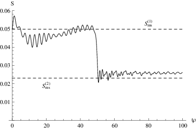


If the mass changes non-adiabatically, this results in a significant particle creation according to the discussion in appendix A. We can thus identify the following regimes:
| (104a) | |||||
| (104b) | |||||
where is given is equation (129b). For the parameters we used in figures 16 and 16 we are in the adiabatic regime ().
In figure 16 we study a mass increase from to (black line). This decreases the phase space area and consequently the entropy decreases, which we depicted in figure 16. Intuitively, a larger mass of the -field reduces the effect of the quantum corrections of the -field. Hence , where is the constant phase space area calculated for from three Fourier integrals as in equation (91). Likewise, corresponds to the phase space area calculated for . The relevant behaviour to compare with is the constant mass phase space evolution for which we also depicted in figure 16 in gray. Clearly, the late time asymptotes of the two functions coincide and we conclude that, also at late times, no entropy has been generated. As we are in the deep adiabatic regime, this is to be expected.
Now let us study the opposite: a mass decrease from to . This is depicted (black line) in figure 16. Clearly, the phase space area increases from to and we plotted the resulting entropy increase in figure 16. Again, we compared this evolution with the phase space area calculated for a constant mass (gray line). As the two asymptotes also coincide in this case, we conclude that no entropy has been generated at late times by the mass change. Of course, it would be very interesting to see what happens when we study the same process in the non-adiabatic regime and we hope to address this question in a future publication.
If we compare the evolution of the entropy in time in these two cases with the free case , the interacting case reveals much more interesting behaviour. Firstly, due to the presence of an environment field, the constant value to which the entropy settles asymptotically is different from zero, unlike the free case. Secondly, a changing mass induces dynamics: the entropy depends on time and evolves from one value to another or vice versa.
VI Conclusion
We apply the decoherence framework to quantum field theory. We consider two scalar fields, one corresponding to a “system field”, the second to an “environment field”, in interaction via a cubic coupling. Here, we consider an environment in its vacuum state () and postpone finite temperature contributions to a future publication. We neglect the backreaction of the environment field on the system field, assuming that the former remains at .
We advocate the following point of view regarding a sensible application of decoherence to quantum field theory: for some observer inaccessible higher order correlators give rise, once neglected, to an increase in entropy of the system. This is inspired by realising that correlators are measured in quantum field theories and that higher order irreducible -point functions are usually perturbatively suppressed. In this work, we assume that our observer is only sensitive to Gaussian correlators and will hence neglect higher order, non-Gaussian correlators. Neglecting the information stored in these higher order correlators, gives rise to an increase of the entropy of the system. If the system initially occupies the minimal area in phase space (characterised by a pure state with ), we numerically calculate the evolution of the entropy in figure 10. Also, we calculate the asymptotic value of the phase space area and the entropy as a function of the coupling , the mass and to which these functions evolve. This increase in entropy can be understood from the system’s tendency to evolve towards the vacuum state of the interacting theory. Even though we do not solve the full 2PI equations at one loop, we have strong numerical evidence that within our approximation scheme, the system evolves towards its correct stationary interacting vacuum state. If the system, however, starts out initially occupying the state characterised by , we observe no further increase in the entropy. Furthermore, we calculate the decoherence rate in equation (102) which charaterises the exponential rate at which the system approaches its stationary state.
Secondly, we study the effect of a time dependent mass of the system field. Now, calculating can only be addressed numerically. Starting out at mixed state initial conditions , we observe an entropy increase (decrease) due to a mass decrease (increase) as depicted in figures 16 and 16, respectively. By comparing with the constant mass evolution for the entropy, we conclude that no additional entropy has been generated asymptotically by the mass jump. As we study mass changes in the deep adiabatic regime, it remains to be investigated whether this statement also holds in the non-adiabatic regime.
We also would like to draw a few somewhat more technical conclusions. It is important to stress that in interacting field theories where memory effects play a crucial role, one cannot just insert initial conditions at some arbitrary finite time , because one then neglects the memory effects existing from the infinite asymptotic past to . In numerical computations however, one has to start at some finite time. We therefore approximate the propagators in the memory integral from the past infinity to by free propagators, inducing a perturbatively suppressed error.
Also, it has not been previously appreciated in the literature that renormalising the vacuum contribution in the Kadanoff-Baym equations can actually significantly change the structure of these equations. In order to properly take account of the renormalised self-mass contribution we had to extract two time derivatives which can readily be seen from equation (64).
Acknowledgements
JFK thanks Jeroen Diederix for many useful suggestions. JFK and TP thank Tomas Janssen and Gerben Stavenga and acknowledge financial support from FOM grant 07PR2522 and from Utrecht University. The authors thank Julien Serreau for many useful comments and for thoroughly reading the manuscript. The authors also gratefully acknowledge the hospitality of the Nordic Institute for Theoretical Physics (NORDITA) during their stay at the “Electroweak Phase Transition” workshop in June 2009.
Appendix A Quantum Effects of a Changing Mass: Free Case
It is interesting to compare our results to a non-trivial exact case: scattering of a changing mass field in the spirit of Birrell and Davies [88]. The solutions presented here stem from the cosmological particle creation literature (based on [109, 110]) and are originally due to Bernard and Duncan [111]. Let us consider the action of a free scalar field:
| (105) |
where as usual is the Minkowski metric, and where we consider the following behaviour of the mass of the scalar field:
| (106) |
From (105), it follows that:
| (107) |
The vacuum causal and statistical propagators follow from (7) and (6) where as:
| (108a) | |||||
| (108b) | |||||
Let us quantise our fields in -dimensions by making use of creation and annihilation operators:
| (109) |
The annihilation operator acts as usual on the vacuum:
| (110a) | |||
| and we impose the following commutation relations: | |||
| (110b) | |||
Hence the equation of motion for the mode functions of , defined by relation (109), follows straightforwardly as:
| (111) |
where . The mode functions determine the causal and statistical propagators from (108) completely:
| (112a) | |||||
| (112b) | |||||
Let us at this point for completeness calculate the constant mass causal and statistical propagators in Fourier space. We just insert a constant mass , rather than a changing one as in equation (106):
| (113a) | |||||
| (113b) | |||||
where . Let us now return to the changing mass case. The physical picture is clear: we would like to study reflection and transmission, i.e.: scattering, of an incoming wave due to the changing mass. Before solving this equation of motion exactly, let us first solve for the asymptotic mode functions to gain intuitive understanding. In the asymptotic past (), equation (111) is solved by:
| (114) |
i.e.: one right-moving or incoming wave with frequency:
| (115) |
In the infinite asymptotic future, the solution necessarily is an appropriately normalised linear superposition of a left- and right-moving wave:
| (116) |
where:
| (117) |
and where:
| (118) |
for a consistent canonical quantisation. In both asymptotic regions we can now immediately calculate the statistical propagator from equation (112b):
| (119a) | |||||
| (119b) | |||||
Using equation (9), we can calculate the area in phase space the in and out states occupy:
| (120a) | |||||
| (120b) | |||||
Hence for the entropy we find:
| (121) |
We conclude that in both asymptotic regions the entropy is zero and no entropy has been generated by changing the mass.


However, we can do better than study the asymptotic behaviour only. Birrell and Davies study cosmological particle creation in section 3.4 of their book [88] in a simple, conveniently chosen cosmological setting. They consider a scale factor as a function of conformal time which behaves as:
| (122) |
This represents an asymptotically static universe with a smooth expansion connecting these two asymptotic regions. Indeed, the equation of motion (in conformal time) for the mode functions Birrell and Davies consider coincides precisely with (111). The solution to (111) which behaves as a positive frequency mode in the asymptotic past () can be expressed in terms of Gauss’ hypergeometric function :
| (123) |
such that:
| (124) |
where we defined and in equations (115) and (117), respectively, and:
| (125) |
Alternatively, the modes which reduce to positive frequency modes in the out region are given by:
| (126) |
such that:
| (127) |
We can rewrite the hypergeometric functions using equations (15.3.3) and (15.3.6) of [112] and identify:
| (128) |
where
| (129a) | |||
| (129b) | |||
Having the mode functions at our disposal, we can find (the rather cumbersome expressions for) the exact causal and statistical propagators. The statistical and causal propagators can however neatly be visualised. Figure 22 shows the causal propagator with a constant mass from equation (113a) for comparison to the changing mass case. In figures 22 and 22 we show the exact causal propagator for a relatively small increase of the mass (from to ) and a larger one (from to ) for one particular Fourier mode only (). Figures 22, 22 and 22 show the analogous statistical propagators.
We can easily relate the statistical propagator to the phase space area by making use of equation (9). It will not come as a surprise to the reader that we find:
| (130) |
and hence:
| (131) |
also for all intermediate times. A final remark is in order. The reader should not confuse calculated from equation (129b) with the phase space particle number density or statistical number density (11). Although the mass is changing, the phase space particle density remains zero but , which in the literature is often referred to as a particle number, can change significantly as can be appreciated from figure 23. This is just caused by the fact that the in and out vacua differ. We plot the behaviour of as a function of in both the adiabatic regime () and non-adiabatic regime ().

This simple example suggests the following: (i) the area in phase space a state occupies is a good quantitative measure of the entropy, (ii) the statistical propagator contains all the information required to calculate this phase space area, and (iii) a changing mass does not change the entropy for a free scalar field. If we contrast this result with the calculations performed in the main body of the paper, it is important to realise that just a changing mass, in the absence of interactions, produces no entropy, whereas we have shown that the entropy can change in the interacting case.
Appendix B Evaluation of the Thermal Propagators
In this appendix, we will for pedagogical reasons derive the thermal propagators from first principles. The four thermal propagators should solve the standard differential equation (19). We start by summarising the conditions the thermal propagators have to satisfy in position space:
| (132a) | |||||
| (132b) | |||||
| (132c) | |||||
| (132d) | |||||
| (132e) | |||||
Here, the first condition (identical to (18c)) and the second relate the sum and the difference of the time ordered and anti-time ordered propagators to the two Wightman functions, respectively. The third condition is just identical to (18d). Condition (132d) is the well-known KMS condition or Kubo-Martin-Schwinger condition, see [113, 114]. The KMS condition corresponds to periodic boundary conditions in the imaginary time direction due to assuming a thermal density matrix operator . The final equation arises from requiring standard commutation relations. Fourier transforming the equations above according to (38) yields:
| (133a) | |||||
| (133b) | |||||
| (133c) | |||||
| (133d) | |||||
| (133e) | |||||
To obtain the second relation (133b), we recall:
| (134) |
where denotes the Cauchy principal value. Relations (133d) and (133e) trivially yield the two thermal Wightman functions:
| (135a) | |||||
| (135b) | |||||
where is the Bose-Einstein distribution given by (42). In order to solve for the time ordered and anti-time ordered propagators, let us make the following general ansätze:
| (136a) | |||||
| (136b) | |||||
The functions and do not depend on due to the delta function. We have already chosen the time ordered and anti-time ordered pole prescription. This is particularly convenient because, as we will appreciate in a moment, this allows us to easily recover the familiar vacuum solutions when . We will return to this subtlety shortly. Condition (133b) immediately implies:
| (137) |
where we have made use of the Dirac identity:
| (138) |
Because of the time ordering, such that . This consideration likewise applies for the anti-time ordered propagator and suggests that the most economic way of writing is in terms of . We observe:
| (139) |
Using the relation above and condition (133a):
| (140) |
The thermal propagators are thus given by:
| (141a) | |||||
| (141b) | |||||
| (141c) | |||||
| (141d) | |||||
If we now let to obtain the familiar vacuum solutions, we find:
| (142a) | |||||
| (142b) | |||||
| (142c) | |||||
| (142d) | |||||
Clearly, writing the thermal propagators in the form (141) above, facilitates obtaining the vacuum solutions easily. The reason is that when , whereas this statement does not hold for .
The freedom to choose a different pole prescription such as the advanced or retarded pole prescription, is just an equivalent way of writing the thermal propagators, which can easily be verified by making use of the Dirac identity (138). The vacuum and thermal contributions to and separate only so neatly when we use the time ordered and anti-time ordered contours to evaluate these propagators, respectively.
Appendix C Alternative Method of Renormalising the Self-masses
In this appendix, we find the correctly renormalised self-masses by means of an alternative Fourier space calculation. From equations (34a) and (43a) we immediately deduce:
| (143) | |||||
where we used Feynman’s trick (see e.g. [115]), performed a Wick rotation and we defined as the new Euclideanised integration variable. The integral can now straightforwardly be performed, which yields when :
| (144) | |||||
where in the last line we have expanded around as usual and we have again introduced a scale to make the argument of the logarithm dimensionless. Observe that the (numerical value of the) divergent term coincides with equation (51) as it should be. Note that for , we would have to use the other Wick rotation (in order not to cross the poles) giving us the desired minus sign difference just as in the position space calculation. Finally, we need to perform the integral in order to derive the self-mass in Fourier space. The relevant integral is:
| (145) | |||||
In order to make the inverse Fourier integral convergent, we introduce regulators where appropriate. As an intermediate result, we present:
| (146) | |||||
Clearly, the regulators in the logarithms and exponents are redundant and can be sent to zero. Using the Dirac rule in equation (138) once more, we finally arrive at:
| (147) |
This result is divergent when we let . As already discussed in the paper in section III, the correct way to deal with this is to extract two time derivatives acting on e.g. . We then remain with a perfectly finite result, which can be appreciated from equation (64).
To prove this, let us indeed evaluate the two time derivatives in equation (64). The result is:
| (148) | |||||
The first line contains two elements. The first is obtained directly from evaluating the double time derivative in equation (64). The second contribution originates from expanding the term multiplying the delta function in equation (51) around , corresponding to the minimal subtraction renormalisation scheme. Indeed, the second line of equation (148) is identical to (147) as it should be. This shows that the position space and Fourier space calculations yield identical results, however the former calculation proves to be superior to the latter as the two extracted time derivatives appear naturally in that case.
Appendix D Retarded Self-mass
The retarded self-mass can be obtained by means of an independent calculation by making use of equation (52):
| (149) | |||||
where as before . In Fourier space we find after some partial integrations:
| (150) | |||||
The last integral is performed in e.g. [116]:
| (151) | |||||
Since the term in square brackets is proportional to as , the commutes through one of the operators. Evaluating it further yields:
| (152) |
If we determine the retarded self-mass directly from equation (64), we find perfect agreement with the result above, representing yet another consistency check of (64).
Appendix E The Statistical Propagator in Fourier Space
Let us now calculate the statistical propagator in Fourier space. Starting point is the equation of motion (39) in Fourier space. We can straightforwardly write the two Wightman functions as:
| (153a) | |||||
| (153b) | |||||
where we have made use of the definition of the advanced propagator (24b) in Fourier space:
| (154) |
Moreover, we made use of:
| (155a) | |||||
| (155b) | |||||
Clearly, we need to evaluate some self-masses in Fourier space. The simplest method of determining e.g. or is to use the retarded self-mass in Fourier space and which we already derived before in appendix C. Using expressions (72) and (152) we can derive:
| (156) | |||||
where and where we have used two partial integrations and disposed ourselves of the boundary terms by introducing an regulator where necessary. We can now use:
| (157) |
and moreover we write:
| (158) |
to prepare for another partial integration. Equation (156) evaluates to:
| (159) | |||||
For , we can use:
| (160) |
to evaluate the remaining integrals. The result is:
| (161) |
From we can immediately find the Wightman self-masses. We take from equation (144), but we have to make sure we use the same subtraction scheme as in our position space calculation in equation (52). We therefore modify equation (144) slightly to:
| (162) |
We thus find:
| (163a) | |||||
| (163b) | |||||
As a check, we consider the following relation that has to be satisfied:
| (164) |
Of course, is given in equation (162) which also allows us to derive the anti-time ordered self-mass:
| (165) |
where contains an additional minus sign because of the Wick rotation (see appendix C for details). We thus find:
| (166) |
This is in perfect agreement with equation (163).
Using equations (153), (162) and (163) we can derive our solutions for the two Wightman functions in Fourier space:
| (167a) | |||||
| (167b) | |||||
The limit in the equations above nicely agrees with the vacuum Wightman propagators in equations (43c) and (43d). Hence the statistical propagator in Fourier space reads:
| (168) | |||||
References
- [1] H. D. Zeh, On the Interpretation of Measurement in Quantum Theory, Found. Phys. 1 (1970) 69.
- [2] W. H. Zurek, Pointer Basis of Quantum Apparatus: Into What Mixture Does the Wave Packet Collapse?, Phys. Rev. D 24 (1981) 1516.
- [3] E. Joos and H. D. Zeh, The Emergence of Classical Properties through Interaction with the Environment, Z. Phys. B 59 (1985) 223.
- [4] W. H. Zurek, Decoherence and the Transition from Quantum to Classical, Phys. Today 44N10 (1991) 36.
- [5] J. B. Hartle, Space-Time Quantum Mechanics and the Quantum Mechanics of Space-Time, arXiv:gr-qc/9304006.
- [6] D. Giulini, C. Kiefer, E. Joos, J. Kupsch, I. O. Stamatescu and H. D. Zeh, Decoherence and the Appearance of a Classical World in Quantum Theory, Springer (second edition, 2003).
- [7] J. P. Paz and W. H. Zurek, Environment-induced Decoherence and the Transition from Quantum to Classical, Lectures given at the 72nd Les Houches Summer School on ‘Coherent Matter Waves’ (1999) quant-ph/0010011.
- [8] W. H. Zurek, Decoherence, Einselection, and the Quantum Origins of the Classical, Rev. Mod. Phys. 75 (2003) 715.
- [9] M. A. Schlosshauer, Decoherence and the Quantum-to-Classical Transition, Springer (2008)
- [10] T. Prokopec, Entropy of the Squeezed Vacuum, Class. Quant. Grav. 10 (1993) 2295.
- [11] R. H. Brandenberger, T. Prokopec and V. F. Mukhanov, The Entropy of the Gravitational Field, Phys. Rev. D 48 (1993) 2443 [arXiv:gr-qc/9208009].
- [12] J. F. Koksma, Decoherence in Quantum Field Theory, Poster and Poster Presentation at the “Trends in Theory” Conference, 14 May 2009, Dalfsen, The Netherlands.
- [13] J. F. Koksma and T. Prokopec, Quantum Reflection in a Thermal Bath, Talk at the “Electroweak Phase Transition” Workshop, 26 June 2009, Nordita, Stockholm, Sweden.
- [14] J. F. Koksma, T. Prokopec and M. G. Schmidt, Entropy and Correlators in Quantum Field Theory, in preparation.
- [15] A. Giraud and J. Serreau, Decoherence and Thermalization of a Pure Quantum State in Quantum Field Theory, arXiv:0910.2570 [hep-ph].
- [16] D. Campo and R. Parentani, Decoherence and Entropy of Primordial Fluctuations II. The Entropy Budget, Phys. Rev. D 78 (2008) 065045 [arXiv:0805.0424 [hep-th]].
- [17] H. T. Elze, Quantum Decoherence, Entropy and Thermalization in Strong Interactions at High-energy. 1: Noisy and Dissipative Vacuum Effects in Toy Models, Nucl. Phys. B 436 (1995) 213 [arXiv:hep-ph/9404215].
- [18] R. H. Brandenberger, R. Laflamme and M. Mijic, Classical Perturbations from Decoherence of Quantum Fluctuations in the Inflationary Universe, Mod. Phys. Lett. A 5 (1990) 2311.
- [19] D. Polarski and A. A. Starobinsky, Semiclassicality and Decoherence of Cosmological Perturbations, Class. Quant. Grav. 13 (1996) 377 [arXiv:gr-qc/9504030].
- [20] J. Lesgourgues, D. Polarski and A. A. Starobinsky, Quantum-to-classical Transition of Cosmological Perturbations for Non-vacuum Initial States, Nucl. Phys. B 497 (1997) 479 [arXiv:gr-qc/9611019].
- [21] C. Kiefer, D. Polarski and A. A. Starobinsky, Quantum-to-classical Transition for Fluctuations in the Early Universe, Int. J. Mod. Phys. D 7 (1998) 455 [arXiv:gr-qc/9802003].
- [22] C. Kiefer and D. Polarski, Emergence of Classicality for Primordial Fluctuations: Concepts and Analogies, Annalen Phys. 7 (1998) 137 [arXiv:gr-qc/9805014].
- [23] C. Kiefer, J. Lesgourgues, D. Polarski and A. A. Starobinsky, The Coherence of Primordial Fluctuations Produced during Inflation, Class. Quant. Grav. 15 (1998) L67 [arXiv:gr-qc/9806066].
- [24] C. Kiefer, Conceptual Issues in Quantum Cosmology, Lect. Notes Phys. 541 (2000) 158 [arXiv:gr-qc/9906100].
- [25] D. Campo and R. Parentani, Inflationary Spectra, Decoherence, and Two-mode Coherent States, Int. J. Theor. Phys. 44 (2005) 1705 [arXiv:astro-ph/0404021].
- [26] D. Campo and R. Parentani, Inflationary Spectra and Partially Decohered Distributions, Phys. Rev. D 72 (2005) 045015 [arXiv:astro-ph/0505379].
- [27] C. P. Burgess, R. Holman and D. Hoover, On the Decoherence of Primordial Fluctuations during Inflation, Phys. Rev. D 77 (2008) 063534 [arXiv:astro-ph/0601646].
- [28] P. Martineau, On the Decoherence of Primordial Fluctuations during Inflation, Class. Quant. Grav. 24 (2007) 5817 [arXiv:astro-ph/0601134].
- [29] D. H. Lyth and D. Seery, Classicality of the Primordial Perturbations, Phys. Lett. B 662 (2008) 309 [arXiv:astro-ph/0607647].
- [30] C. Kiefer, I. Lohmar, D. Polarski and A. A. Starobinsky, Pointer States for Primordial Fluctuations in Inflationary Cosmology, Class. Quant. Grav. 24 (2007) 1699 [arXiv:astro-ph/0610700].
- [31] T. Prokopec and G. I. Rigopoulos, Decoherence from Isocurvature Perturbations in Inflation, JCAP 0711 (2007) 029 [arXiv:astro-ph/0612067].
- [32] J. W. Sharman and G. D. Moore, Decoherence due to the Horizon after Inflation, JCAP 0711 (2007) 020 [arXiv:0708.3353 [gr-qc]].
- [33] C. Kiefer, I. Lohmar, D. Polarski and A. A. Starobinsky, Origin of Classical Structure in the Universe, J. Phys. Conf. Ser. 67 (2007) 012023.
- [34] D. Campo and R. Parentani, Decoherence and Entropy of Primordial Fluctuations. I: Formalism and Interpretation, Phys. Rev. D 78 (2008) 065044 [arXiv:0805.0548 [hep-th]].
- [35] C. Kiefer and D. Polarski, Why do Cosmological Perturbations Look Classical to Us?, arXiv:0810.0087 [astro-ph].
- [36] D. Sudarsky, Shortcomings in the Understanding of Why Cosmological Perturbations Look Classical, arXiv:0906.0315 [gr-qc].
- [37] F. Lombardo and F. D. Mazzitelli, Coarse Graining and Decoherence in Quantum Field Theory, Phys. Rev. D 53 (1996) 2001 [arXiv:hep-th/9508052].
- [38] F. C. Lombardo, F. D. Mazzitelli and R. J. Rivers, Decoherence in Field Theory: General Couplings and Slow Quenches, Nucl. Phys. B 672 (2003) 462 [arXiv:hep-ph/0204190].
- [39] F. C. Lombardo and D. Lopez Nacir, Decoherence during Inflation: The Generation of Classical Inhomogeneities, Phys. Rev. D 72 (2005) 063506 [arXiv:gr-qc/0506051].
- [40] S. Habib, Stochastic Inflation: the Quantum Phase Space Approach, Phys. Rev. D 46 (1992) 2408 [arXiv:gr-qc/9208006].
- [41] A. A. Starobinsky and J. Yokoyama, Equilibrium State of a Selfinteracting Scalar Field in the de Sitter Background, Phys. Rev. D 50 (1994) 6357 [arXiv:astro-ph/9407016].
- [42] O. E. Buryak, Stochastic Dynamics of Large Scale Inflation in de Sitter Space, Phys. Rev. D 53 (1996) 1763 [arXiv:gr-qc/9502032].
- [43] H. Casini, R. Montemayor and P. Sisterna, Stochastic Approach to Inflation. II: Classicality, Coarse-graining and Noises, Phys. Rev. D 59 (1999) 063512 [arXiv:gr-qc/9811083].
- [44] E. A. Calzetta, B. L. Hu and F. D. Mazzitelli, Coarse-grained Effective Action and Renormalization Group Theory in Semiclassical Gravity and Cosmology, Phys. Rept. 352 (2001) 459 [arXiv:hep-th/0102199].
- [45] J. Martin and M. A. Musso, Stochastic quintessence, Phys. Rev. D 71 (2005) 063514 [arXiv:astro-ph/0410190].
- [46] N. C. Tsamis and R. P. Woodard, Stochastic Quantum Gravitational Inflation, Nucl. Phys. B 724 (2005) 295 [arXiv:gr-qc/0505115].
- [47] E. Calzetta and B. L. Hu, Quantum Fluctuations, Decoherence of the Mean Field, and Structure Formation in the Early Universe, Phys. Rev. D 52 (1995) 6770 [arXiv:gr-qc/9505046].
- [48] J. Berges, Introduction to Nonequilibrium Quantum Field Theory, AIP Conf. Proc. 739 (2005) 3 [arXiv:hep-ph/0409233].
- [49] J. Berges and S. Borsanyi, Progress in Nonequilibrium Quantum Field Theory. III, Nucl. Phys. A 785 (2007) 58 [arXiv:hep-ph/0610015].
- [50] G. Aarts and J. Berges, Nonequilibrium Time Evolution of the Spectral Function in Quantum Field Theory, Phys. Rev. D 64 (2001) 105010 [arXiv:hep-ph/0103049].
- [51] J. Berges, Controlled Nonperturbative Dynamics of Quantum Fields out of Equilibrium, Nucl. Phys. A 699, 847 (2002) [arXiv:hep-ph/0105311].
- [52] G. Aarts and J. Berges, Classical Aspects of Quantum Fields far from Equilibrium, Phys. Rev. Lett. 88 (2002) 041603 [arXiv:hep-ph/0107129].
- [53] G. Aarts, D. Ahrensmeier, R. Baier, J. Berges and J. Serreau, Far-from-equilibrium Dynamics with Broken Symmetries from the 2PI-1/N Expansion, Phys. Rev. D 66 (2002) 045008 [arXiv:hep-ph/0201308].
- [54] J. Berges and J. Serreau, Parametric Resonance in Quantum Field Theory, Phys. Rev. Lett. 91 (2003) 111601 [arXiv:hep-ph/0208070].
- [55] S. Juchem, W. Cassing and C. Greiner, Quantum Dynamics and Thermalization for Out-of-equilibrium -theory, Phys. Rev. D 69 (2004) 025006 [arXiv:hep-ph/0307353].
- [56] S. Juchem, W. Cassing and C. Greiner, Nonequilibrium Quantum-field Dynamics and Off-shell Transport for phi**4-theory in 2+1 Dimensions, Nucl. Phys. A 743 (2004) 92 [arXiv:nucl-th/0401046].
- [57] A. Arrizabalaga, J. Smit and A. Tranberg, Tachyonic Preheating using 2PI - 1/N Dynamics and the Classical Approximation, JHEP 0410 (2004) 017 [arXiv:hep-ph/0409177].
- [58] A. Arrizabalaga, J. Smit and A. Tranberg, Equilibration in phi**4 Theory in 3+1 Dimensions, Phys. Rev. D 72 (2005) 025014 [arXiv:hep-ph/0503287].
- [59] J. Berges, S. Borsanyi and J. Serreau, Thermalization of Fermionic Quantum Fields, Nucl. Phys. B 660 (2003) 51 [arXiv:hep-ph/0212404].
- [60] A. Anisimov, W. Buchmuller, M. Drewes and S. Mendizabal, Nonequilibrium Dynamics of Scalar Fields in a Thermal Bath, Annals Phys. 324 (2009) 1234 [arXiv:0812.1934 [hep-th]].
- [61] E. A. Calzetta and B. L. Hu, Thermalization of an Interacting Quantum Field in the CTP-2PI Next-to-leading-order Large N Scheme, arXiv:hep-ph/0205271.
- [62] E. A. Calzetta and B. L. Hu, Correlation Entropy of an Interacting Quantum Field and H-theorem for the O(N) Model, Phys. Rev. D 68 (2003) 065027 [arXiv:hep-ph/0305326].
- [63] H. van Hees and J. Knoll, Renormalization in Self-consistent Approximations Schemes at Finite Temperature. I: Theory, Phys. Rev. D 65 (2002) 025010 [arXiv:hep-ph/0107200].
- [64] H. Van Hees and J. Knoll, Renormalization of Self-consistent Approximation Schemes. II: Applications to the Sunset Diagram, Phys. Rev. D 65 (2002) 105005 [arXiv:hep-ph/0111193].
- [65] H. van Hees and J. Knoll, Renormalization in Self-consistent Approximation Schemes at Finite Temperature. III: Global Symmetries, Phys. Rev. D 66 (2002) 025028 [arXiv:hep-ph/0203008].
- [66] J. Berges, S. Borsanyi, U. Reinosa and J. Serreau, Nonperturbative Renormalization for 2PI Effective Action Techniques, Annals Phys. 320 (2005) 344 [arXiv:hep-ph/0503240].
- [67] S. Borsanyi and U. Reinosa, Renormalised Nonequilibrium Quantum Field Theory: Scalar Fields, Phys. Rev. D 80 (2009) 125029 [arXiv:0809.0496 [hep-th]].
- [68] S. Borsanyi and U. Reinosa, Renormalisation of out-of-equilibrium Quantum Fields, Nucl. Phys. A 820 (2009) 147C.
- [69] J. P. Blaizot, E. Iancu and U. Reinosa, Renormalization of Phi-derivable Approximations in Scalar Field Theories, Nucl. Phys. A 736 (2004) 149 [arXiv:hep-ph/0312085].
- [70] J. P. Blaizot, E. Iancu and U. Reinosa, Renormalizability of Phi-derivable Approximations in Scalar phi**4 Theory, Phys. Lett. B 568 (2003) 160 [arXiv:hep-ph/0301201].
- [71] H. Collins and R. Holman, Taming the Alpha Vacuum, Phys. Rev. D 70 (2004) 084019 [arXiv:hep-th/0312143].
- [72] H. Collins and R. Holman, Renormalization of Iinitial Conditions and the Trans-Planckian Problem of Inflation, Phys. Rev. D 71 (2005) 085009 [arXiv:hep-th/0501158].
- [73] H. Collins and R. Holman, The Renormalization of the Energy-momentum Tensor for an Effective Initial State, Phys. Rev. D 74 (2006) 045009 [arXiv:hep-th/0605107].
- [74] H. Collins and R. Holman, The Energy-momentum Tensor for an Effective Initial State and the Renormalization of Gravity, arXiv:hep-th/0609002.
- [75] M. Garny and M. M. Muller, Kadanoff-Baym Equations with Non-Gaussian Initial Conditions: The Equilibrium Limit, arXiv:0904.3600 [hep-ph].
- [76] B. Garbrecht, T. Prokopec and M. G. Schmidt, Coherent baryogenesis, Phys. Rev. Lett. 92 (2004) 061303 [arXiv:hep-ph/0304088].
- [77] B. Garbrecht, T. Prokopec and M. G. Schmidt, Coherent Baryogenesis and Nonthermal Leptogenesis: a Comparison, arXiv:hep-ph/0410132.
- [78] B. Garbrecht, T. Prokopec and M. G. Schmidt, SO(10) - GUT coherent baryogenesis, Nucl. Phys. B 736 (2006) 133 [arXiv:hep-ph/0509190].
- [79] G. R. Farrar and M. E. Shaposhnikov, Baryon Asymmetry of the Universe in the Standard Electroweak Theory, Phys. Rev. D 50 (1994) 774 [arXiv:hep-ph/9305275].
- [80] G. R. Farrar and M. E. Shaposhnikov, Baryon Asymmetry of the Universe in the Minimal Standard Model, Phys. Rev. Lett. 70 (1993) 2833 [Erratum-ibid. 71 (1993) 210] [arXiv:hep-ph/9305274].
- [81] M. B. Gavela, P. Hernandez, J. Orloff and O. Pene, Standard Model CP-violation and Baryon asymmetry, Mod. Phys. Lett. A 9 (1994) 795 [arXiv:hep-ph/9312215].
- [82] P. Huet and E. Sather, Electroweak Baryogenesis and Standard Model CP Violation, Phys. Rev. D 51 (1995) 379 [arXiv:hep-ph/9404302].
- [83] M. B. Gavela, M. Lozano, J. Orloff and O. Pene, Standard Model CP Violation and Baryon Asymmetry. Part 1: Zero Temperature, Nucl. Phys. B 430 (1994) 345 [arXiv:hep-ph/9406288].
- [84] M. B. Gavela, P. Hernandez, J. Orloff, O. Pene and C. Quimbay, Standard Model CP Violation and Baryon Asymmetry. Part 2: Finite Temperature, Nucl. Phys. B 430 (1994) 382 [arXiv:hep-ph/9406289].
- [85] M. Herranen, K. Kainulainen and P. M. Rahkila, Quantum Kinetic Theory for Fermions in Temporally Varying Backrounds, JHEP 0809 (2008) 032 [arXiv:0807.1435 [hep-ph]].
- [86] M. Herranen, K. Kainulainen and P. M. Rahkila, Towards a Kinetic Theory for Fermions with Quantum Coherence, Nucl. Phys. B 810 (2009) 389 [arXiv:0807.1415 [hep-ph]].
- [87] M. Herranen, K. Kainulainen and P. M. Rahkila, Kinetic Theory for Scalar Fields with Nonlocal Quantum Coherence, JHEP 0905 (2009) 119 [arXiv:0812.4029 [hep-ph]].
- [88] N. D. Birrell and P. C. W. Davies, Quantum Fields in Curved Space, Cambridge monographs on Mathematical Physics, Cambridge University Press (1982).
- [89] J. S. Schwinger, Brownian Motion of a Quantum Oscillator, J. Math. Phys. 2 (1961) 407.
- [90] L. V. Keldysh, Diagram Technique for Nonequilibrium Processes, Zh. Eksp. Teor. Fiz. 47 (1964) 1515 [Sov. Phys. JETP 20 (1965) 1018].
- [91] K. c. Chou, Z. b. Su, B. l. Hao and L. Yu, Equilibrium and Nonequilibrium Formalisms Made Unified, Phys. Rept. 118 (1985) 1.
- [92] R. D. Jordan, Effective Field Equations for Expectation Values, Phys. Rev. D 33 (1986) 444.
- [93] E. Calzetta and B. L. Hu, Nonequilibrium Quantum Fields: Closed Time Path Effective Action, Wigner Function and Boltzmann Equation, Phys. Rev. D 37 (1988) 2878.
- [94] S. Weinberg, Quantum Contributions to Cosmological Correlations, Phys. Rev. D 72 (2005) 043514 [arXiv:hep-th/0506236].
- [95] J. F. Koksma, T. Prokopec and G. I. Rigopoulos, The Scalar Field Kernel in Cosmological Spaces, Class. Quant. Grav. 25 (2008) 125009 [arXiv:0712.3685 [gr-qc]].
- [96] T. Prokopec, M. G. Schmidt and S. Weinstock, Transport Equations for Chiral Fermions to Order h-bar and Electroweak Baryogenesis, Annals Phys. 314 (2004) 208 [arXiv:hep-ph/0312110].
- [97] M. van der Meulen and J. Smit, Classical Approximation to Quantum Cosmological Correlations, JCAP 0711 (2007) 023 [arXiv:0707.0842 [hep-th]].
- [98] J. M. Cornwall, R. Jackiw and E. Tomboulis, Effective Action For Composite Operators, Phys. Rev. D 10, 2428 (1974).
- [99] R. Jackiw, Functional Evaluation of the Effective Potential, Phys. Rev. D 9 (1974) 1686.
- [100] L. P. Kadanoff and G. Baym, Quantum Statistical Mechanics, Benjamin Press, New York (1962).
- [101] M. Le Bellac, Thermal Field Theory, Cambridge monographs on Mathematical Physics, Cambridge University Press (1996).
- [102] I. S. Gradshteyn and I. M. Ryzhik, Table of Integrals, Series and Products, Academic Press (1965).
- [103] T. M. Janssen, S. P. Miao, T. Prokopec and R. P. Woodard, Infrared Propagator Corrections for Constant Deceleration, Class. Quant. Grav. 25 (2008) 245013 [arXiv:0808.2449 [gr-qc]].
- [104] T. Janssen and T. Prokopec, A Graviton Propagator for Inflation, Class. Quant. Grav. 25 (2008) 055007 [arXiv:0707.3919 [gr-qc]].
- [105] T. Janssen, S. P. Miao and T. Prokopec, Graviton One-loop Effective Action and Inflationary Dynamics, arXiv:0807.0439 [gr-qc].
- [106] S. P. Miao and R. P. Woodard, Gravitons Enhance Fermions during Inflation, Phys. Rev. D 74 (2006) 024021 [arXiv:gr-qc/0603135].
- [107] J. Serreau, Out-of-Equilibrium Electromagnetic Radiation, JHEP 0405 (2004) 078 [arXiv:hep-ph/0310051].
- [108] H. A. Weldon, Simple Rules for Discontinuities in Finite Temperature Field Theory, Phys. Rev. D 28 (1983) 2007.
- [109] L. Parker, Particle Creation in Expanding Universes, Phys. Rev. Lett. 21 (1968) 562.
- [110] L. Parker, Quantized Fields and Particle Creation in Expanding Universes. 1, Phys. Rev. 183, 1057 (1969).
- [111] C. W. Bernard and A. Duncan, Regularization and Renormalization of Quantum Field Theory in Curved Space-Time, Annals Phys. 107 (1977) 201.
- [112] M. Abramowitz and I. A. Stegun, Handbook of Mathematical Functions, Dover Publications (1965).
- [113] R. Kubo, Statistical Mechanical Theory of Irreversible Processes. 1. General Theory and Simple Applications in Magnetic and Conduction Problems, J. Phys. Soc. Jap. 12 (1957) 570.
- [114] P. C. Martin and J. S. Schwinger, Theory of Many Particle Systems. I, Phys. Rev. 115 (1959) 1342.
- [115] M. E. Peskin and D. V. Schroeder, An Introduction to Quantum Field Theory, Westview Press (1995)
- [116] T. Prokopec, O. Tornkvist and R. P. Woodard, One Loop Vacuum Polarization in a Locally de Sitter Background, Annals Phys. 303 (2003) 251 [arXiv:gr-qc/0205130].