Distinguishing Cause and Effect via Second Order Exponential Models

A simple case where cause and effect is identifiable in our model class is already given by the motivating example with a binary variable $X$ and a variable $Y$ that can attain all values in $\mathbb{R}$.

Using both equations (2), we obtain

$$p(x=1)=\gamma\quad\quad p(y|x=j)=\frac{1}{\sqrt{2\pi}\rho}e^{-\frac{(y-\nu_{j})^{2}}{2\rho^{2}}}\,,$$

(5)

with parameters $\gamma,\nu_{0},\nu_{1},\rho$. Both distributions $p(y|x=j)$ for $j=0,1$ are obviously Gaussians with equal width and different mean, i.e., $p(y)$ is a mixture of two Gaussians (see Fig. 1, left).

We obtain

$$p(y)=\frac{1}{\sqrt{2\pi}\sigma}e^{-\frac{(y-\nu)^{2}}{2\sigma^{2}}}\quad\quad p(x=1|y)=\frac{1}{2}\big(1+\tanh(\alpha y+\beta)\big)\,,$$

(6)

with parameters $\nu,\sigma,\alpha,\beta$, where we have used

$$\frac{e^{a}}{1+e^{a}}=\frac{1}{e^{-a}+1}=\frac{1}{2}(1+\tanh(a/2))\,.$$

(7)

A typical joint distribution for the model $Y\rightarrow X$ is shown in Fig. 3.

Since mixtures of two different Gaussians can never yield a Gaussian as marginal distribution $p(y)$, the only joint distribution that is contained in the model classes for both directions is a product distribution of a Gaussian $p(y)$ and an arbitrary binary distribution $p(x)$. This shows that the models are identifiable except for the trivial case of independence.

Furthermore, eqs. (5) and (6) show that our method is indeed consistent with the intuitive arguments we gave for the examples in the introduction: the Gaussian mixture in Fig. 1 is a second order model for $X\rightarrow Y$ and the example with thresholding $y$ (Fig. 2) can be approximated by second order models for $Y\rightarrow X$ via the limit $\alpha\to\infty$ in eq. (6).

We first simplify equation (2) for the case that all variables $X_{1},\dots,X_{n}$ are binary. Writing $an_{j}:=x_{1},\dots,x_{j-1}$ for the ancestors of $x_{j}$, we obtain

$$p(x_{j}=1|an_{j})=\frac{\exp(\alpha_{j}+\beta_{jj}+\sum_{i<j}\beta_{ji}x_{i})}{1+\exp(\alpha_{j}+\beta_{jj}+\sum_{i<j}\beta_{ji}x_{i})}\,.$$

Using eq. (7) yields

$$p(x_{j}=1|an_{j})=\frac{1}{2}\big(1+\tanh(\lambda_{j}+\sum_{i=1}^{j-1}\lambda_{ji}x_{i})\big)\,.$$

(8)

with

$$\lambda_{j}:=\frac{1}{2}\left(\alpha_{j}+\beta_{jj}\right)\quad\mbox{and}\quad\lambda_{ji}=\frac{1}{2}\beta_{ij}\quad\mbox{ for }\quad i=1,\dots,j-1\,.$$

The joint distributions induced by these conditionals do not coincide for all causal orders provided that $n\geq 4$. To show this, we first observe that second order models can approximate the causal relation between the inputs and the output of an $(n-1)$-bit OR gate. Then we show that the conditional probability for one input, given the other $n-2$ inputs and the output is significantly more complex than a second order model since it requires polynomials of degree $n-2$ as argument of the $\tanh$-function (which corresponds to polynomials of degree $n-1$ in the exponent in the same way as second order models lead to linear arguments of $\tanh$).

The OR gate with input $X_{1},\dots,X_{n-1}$ and output $X_{n}$ is described by

$$p(x_{n}=1|an_{n})=1-\prod_{i=1}^{n-1}(1-x_{i})\,.$$

Introducing a sequence of second order conditionals by

$$p_{k}(x_{n}=1|an_{n}):=\frac{1}{2}\big(1+\tanh(-k+2k\sum_{i=1}^{n-1}x_{i})\big)\,,$$

we have

$$\lim_{k\to\infty}p_{k}(x_{n}|an_{n})=p(x_{n}|an_{n})\,,$$

and thus they approximate the OR-gate.

Let the inputs $X_{1},\dots,X_{n-1}$ be sampled from the uniform distribution over $\{0,1\}^{n-1}$. We then have

$$p\left(x_{1}=1|x_{2},x_{3},\dots,x_{n-1},x_{n}=1\right)=\left\{\begin{array}[]{cl}1&\mbox{for}\,x_{2}=x_{3}=\cdots=x_{n-1}=0\\ \frac{1}{2}&\mbox{otherwise}\end{array}\right.$$

(9)

and

$$p\left(x_{1}=1|x_{2}=\cdots=x_{n}=0\right)=0\,.$$

(10)

Note that the event $X_{n}=0$ and $X_{i}=1$ for some $i\in\left\{2,\ldots,n-1\right\}$ does not occur and the corresponding conditional probabilities need not to be specified.

We now show that the joint distribution cannot be approximated by second order models if $X_{n}$ is not the last node. For symmetry reasons, it is sufficient to show that $p(x_{1}|x_{2},\dots,x_{n})$ has no second order model approximation. If such an approximation existed, we would have

$$p\left(x_{1}=1|x_{2},\dots,x_{n}\right)=\lim_{k\to\infty}\frac{1}{2}\Big(1+\tanh\big(q_{k}(x_{2},\ldots,x_{n}\big))\Big)\,,$$

(11)

where $q_{k}$ is a sequence of linear functions in $x_{2},\dots,x_{n}$, see eq. (8). We prove that eq. (11) can indeed be satisfied with $q_{k}$ of polynomials of order $n-2$, but not for any sequence of polynomials of lower order (which shows that these non-causal conditional can be rather complex). Introducing

$$\tilde{q}_{k}(x_{2},\dots,x_{n-1}):=q_{k}(x_{2},\dots,x_{n-1},x_{n}=1)\,,$$

eq. (9) is equivalent to

$$\lim_{k\to\infty}\tilde{q}_{k}(x_{2},\dots,x_{n-1},x_{n}=1)=\left\{\begin{array}[]{cl}\infty&\mbox{for}\,x_{2}=x_{3}=\cdots=x_{n-1}=0\\ 0&\mbox{otherwise}\end{array}\right.$$

(12)

If the space of polynomials of degree $n-3$ or lower contained such a sequence $\tilde{q}_{k}$ , completeness of finite dimensional real vector spaces implies that it also contained

$$g:=\lim_{k\to\infty}\frac{1}{\|\tilde{q}_{k}\|_{1}}\tilde{q}_{k}\,,$$

which is given by

$$g\left(x_{2},\ldots,x_{n-1}\right)=\left\{\begin{array}[]{cl}1&\mbox{for}\,x_{2}=x_{3}=\cdots=x_{n-1}=0\\ 0&\mbox{otherwise}\,.\end{array}\right.$$

However,

$$g\left(x_{2},\ldots,x_{n-1}\right)=\prod_{i=2}^{n-1}\left(1-x_{i}\right)\,,$$

which is a polynomial of degree $n-2$. Hence, $\tilde{q}_{k}$ (and also $q_{k}$) consists at least of polynomials of order $n-2$. To see that this bound is tight, set

$$q_{k}(x_{2},\dots,x_{n}):=k\left(2(x_{n}-1)-\prod_{i=2}^{n-1}(1-x_{i})\right)\,,$$

and observe that it satisfies eq. (12) and

$$\lim_{k\to\infty}q_{k}(x_{2}=0,\dots,x_{n}=0)=-\infty\,,$$

and thus the corresponding conditionals satisfy asymptotically eqs.(9) and (10).

By inverting logical values, the same proof applies to AND gates. Since AND and OR gates are reasonable models for many causal relations in real-life, it is remarkable that the corresponding non-causal conditionals of the generated joint distribution already require exponential models of high order. Successful experiments with artificial and real-world data with four binary variables are briefly sketched in [21].

Since second order models provide a simple class of non-trivial conditional densities, Occam’s Razor seems to strongly support the principle of preferring the direction that admits such a model. However, Occam’s Razor cannot justify why we should try to find simple expressions for the causal conditional $P({\tt effect}|{\tt cause})$ instead of simple models for non-causal conditionals like $P({\tt cause}|{\tt effect})$. Here we present a justification that is based on recent algorithmic information theory based approaches to causal inference.

[15] proposed to prefer those DAGs as causal hypotheses for which the shortest description of the joint density $p(x_{1},\dots,x_{n})$ is given by separate descriptions of causal conditionals $p(x_{j}|pa_{j})$ in eq. (1). We will refer to this as the principle of independent conditionals (IC). Here, the description length is measured in terms of algorithmic information [22, 23, 24], sometimes also called “Kolmogorov complexity”. Even though it is hard to give a precise meaning to this principle, it provides the leading motivation for our theory.

To show this, we reconsider one of the examples from the introduction. We have argued that the distribution in Fig. 2 is unlikely to be generated by the causal structure $X\rightarrow Y$ because the observed distribution $p(x)$ is special among all possible $\tilde{p}(x)$ since it is the only distribution that yields a Gaussian marginal $p(y)$ after feeding it into the conditional $p(y|x)$. Hence, after knowing $p(y|x)$, the input distribution $p(x)$ is simply described by “the unique input that renders $p(y)$ Gaussian”. Thus, a description for $p(x,y)$ that contains separate descriptions of $p(y|x)$ and $p(x)$ would contain redundant information and the IC principle would be fail. We propose a slightly modified version of IC that will be more convenient to use because it refers to algorithmic dependences between unconditional distributions:

The idea is that $\tilde{p}(x,y)$ only contains algorithmic information about $p(y|x)$ and $\tilde{p}(x)$. The object $p(y|x)$ has been chosen independently of $p(x)$ “by nature”, as in [15], and $\tilde{p}(x)$ has been chosen independently of $p(y|x)$ by assumption.

Due to the lack of a precise meaning of the concept of “algorithmic information of probability densities”, as it would be required by [15] and our modified postulate, we will describe arguments that avoid such concepts but still rely on the above intuition.

We therefore rephrase the probability-free approach to causal inference developed by [16]. The idea is that causal inference in real life often does not rely on statistical dependences. Instead, similarities between single objects indicate causal relations. Observing, for instance, that two carpets contain the same patterns makes us believe that designers have copied from each other (provided that the patterns are complex and not common). [16] develop a general framework for inferring causal graphs that connect individual objects based upon algorithmic dependences. Here, two objects are called algorithmically independent if their shortest joint description is given by the concatenations of their separate descriptions. It is assumed that every such description is a binary string $s$ formalizing all relevant properties of an observation. Then the Kolmogorov complexity $K(s)$ of $s$ is defined by the length of the shortest program that generates the output $s$ and then stops. Conditional Kolmogorov complexity $K(s|t)$ is defined as the length of the shortest program that computes $s$ from the input $t$. If $t^{*}$ denotes the shortest compression of $t$, $K(s|t^{*})$ can be smaller than $K(s|t)$ because there is no algorithmic way to obtain the shortest compression (the difference between $K(s|t)$ and $K(s|t^{*})$ can at most be logarithmic in the length of $t$ [25]).

The strings $s$ and $t$ are conditionally independent, given $r$ if

$$K(s,t|r)\approx K(s|r)+K(t|r)\,.$$

(13)

As in the statistical setting, unconditional depedences indicate causal links between two objects $s$ and $t$: if $K(s,t)\ll K(s)+K(t)\,,$ the descriptions can be better compressed jointly than independently and we postulate a causal connection. The following terminology [26] will be crucial:

To also infer causal directions we have postulated a causal Markov condition stating conditional independence of every object from its non-effects, given its causes. We will here state an equivalent version (see Theorem 3 in [16]):

Based on the above framework and inspired by the IC-principle, [16] describe the following approach to distinguishing between $X\rightarrow Y$ and $Y\rightarrow X$ for two random variables $X,Y$ after observing the samples $(x_{1},y_{1}),\dots,(x_{k},y_{k})$. One considers the causal structure among $2k+2$ individual objects instead of a DAG with the two variables as nodes. These objects are: The $x$-values, the $y$-values, the source $S$ emitting $x$-values according to $p(x)$ and a machine emitting $y$-values according to $p(y|x)$. The causal DAG connecting the objects is shown in Fig. 4, left. One may wonder why there are no arrows from the $x$-values to $M$ even though $M$ gets them as inputs. The reason is that the object $M$ is not changed by the $x_{j}$, i.e., the conditional $p(y|x)$ remains constant.

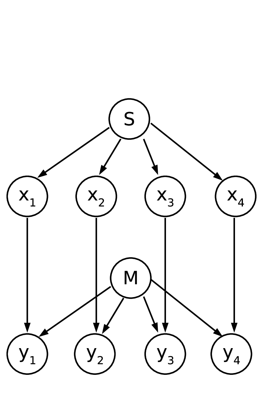
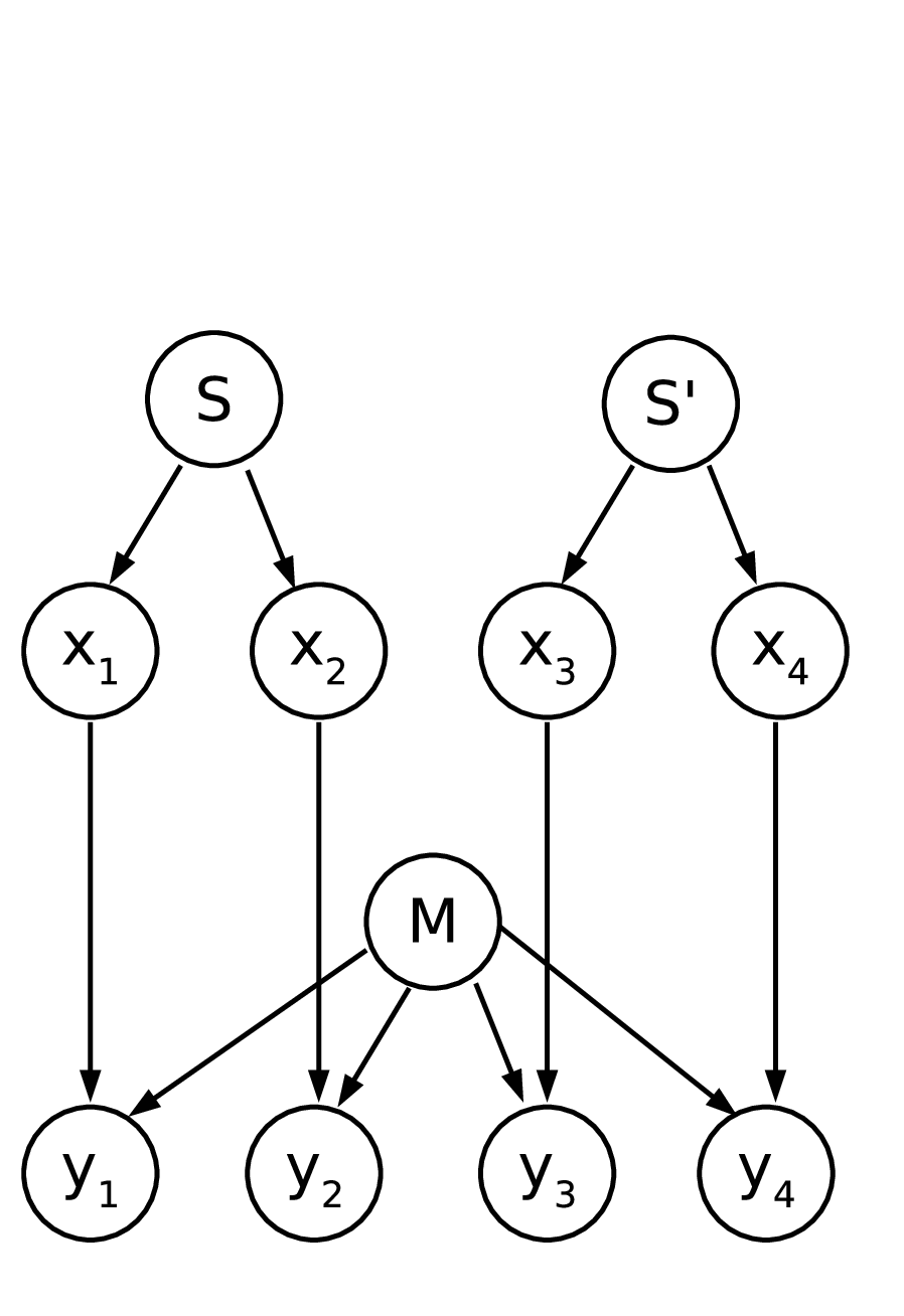
It has been pointed out [16] that the DAG in Fig. 4, left, already imposes the algorithmic independence relation

$$x_{1},\dots,x_{m}\mathchoice{\mathrel{\hbox to0.0pt{$\displaystyle\perp$\hss}\mkern 2.0mu{\displaystyle\perp}}}{\mathrel{\hbox to0.0pt{$\textstyle\perp$\hss}\mkern 2.0mu{\textstyle\perp}}}{\mathrel{\hbox to0.0pt{$\scriptstyle\perp$\hss}\mkern 2.0mu{\scriptstyle\perp}}}{\mathrel{\hbox to0.0pt{$\scriptscriptstyle\perp$\hss}\mkern 2.0mu{\scriptscriptstyle\perp}}}y_{m+1},\dots,y_{k}\,|(x_{m+1},\dots,x_{k})^{*}\quad\quad\forall m<k\,,$$

(14)

and describes examples where this is violated after exchanging the role of $X$ and $Y$. This is an observable implication of the algorithmic independence of the unobservable objects $S$ and $M$. The relevant information about $S$ and $M$ is given by $p(x)$ and $p(y|x)$, respectively, hence condition (14) is closely linked to Lemeire’s and Dirkx’s postulate. [16] discusses toy examples for which the destinction between $X\rightarrow Y$ and $Y\rightarrow X$ is possible using condition (14).

For our purposes, it will be more convenient to work with a slightly different condition that can be seen as a finite-sample counterpart of Postulate 1. To this end, we consider Fig. 4, right. Let ${\bf x}^{1}:=x_{1},\dots,x_{m}$ be the sample of $x$-values from source $S$ (here $m=2$). ${\bf x}^{2}:=x_{m+1},\dots,x_{k}$ denote the $x$-values from source $S^{\prime}$ and ${\bf y}^{2}$ the corresponding $y$-values. The d-separation criterion yields the unconditional relation

$${\bf x}^{1}\mathchoice{\mathrel{\hbox to0.0pt{$\displaystyle\perp$\hss}\mkern 2.0mu{\displaystyle\perp}}}{\mathrel{\hbox to0.0pt{$\textstyle\perp$\hss}\mkern 2.0mu{\textstyle\perp}}}{\mathrel{\hbox to0.0pt{$\scriptstyle\perp$\hss}\mkern 2.0mu{\scriptstyle\perp}}}{\mathrel{\hbox to0.0pt{$\scriptscriptstyle\perp$\hss}\mkern 2.0mu{\scriptscriptstyle\perp}}}{\bf x}^{2},{\bf y}^{2}\,.$$

(15)

Of course, we do not assume that we have the option to really change the input distribution from $p(x)$ to $\tilde{p}(x)$ (i.e., replacing the source $S$ with $S^{\prime}$), otherwise we could directly test whether $X$ causes $Y$ by observing whether such an intervention also changes $p(y)$. Our way of reasoning will be indirect: given that the true causal structure is $X\rightarrow Y$, we could simulate the effect of the intervention by choosing a subsample of $x$-values that is distributed according to $\tilde{p}(x)$ and know that the corresponding pairs $(x,y)$ are distributed according to $p(y|x)\tilde{p}(x)$.

We now describe the violation of condition (15) for the example in Fig. 2. The true model $Y\rightarrow X$ involves the parameters $\nu$, $\sigma$, and $\beta$ (mean and standard deviation of the Gaussian and threshold of $y$-values for which $x=1$). We denote the corresponding density therefore by $p_{\nu,\sigma,\beta}$. Now we consider the non-causal conditional $p_{\nu,\sigma,\beta}(y|x)$. One checks easily that different triples $(\nu,\sigma,\beta)$ indeed induce different $p(y|x)$. On the other hand, there is a unique input probability $p_{\gamma}(x=1)=\gamma$ such that the marginal

$$p_{\gamma,\nu,\sigma,\beta}(y):=\sum_{x}p_{\gamma}(x)p_{\nu,\sigma,\beta}(y|x)$$

is Gaussian:

$$\gamma=f(\nu,\sigma,\beta):=\frac{1}{\sqrt{2\pi}\sigma}\int^{\beta}_{-\infty}e^{-\frac{(y-\nu)^{2}}{2\sigma^{2}}}dy\,.$$

(16)

The fact that $f$ that does not involve any free parameters would already be in contradiction with Lemeire’s and Dirkx’s postulate if $X\rightarrow Y$ were true because $f$ only has constant description length and the parameters can be described with arbitrary accuracy. For sufficiently large accuracy, the description length of $\gamma$ thus exceeds the length of $f$ and eq. (16) provides a shorter description for $\gamma$ than its explicit binary representation.

According to our finite-sample point of view, the parameters $\gamma,\nu,\sigma,\beta$ must only be described up to an accuracy that corresponds to the error made when estimating them from a finite sample: Observing ${\bf x}^{1}$, i.e., an ensemble of $x$-values drawn from $p(x)$, we can estimate $\gamma$ up to a certain accuracy. Similarly, we estimate $\nu,\sigma,\beta$ after observing ${\bf x}^{2},{\bf y}^{2}$ up to a certain accuracy. Then, the estimator for $\mu$ and the estimator of the other parameters will approximately satisfy the functional relation (16). This shows that ${\bf x}^{1}$, on the one hand, and ${\bf x}^{2},{\bf y}^{2}$ on the other hand, share at least that amount of algorithmic information shared by the estimators because the latter have only processed the information contained in the observations.

For general second order models, the argument reads as follows. For $Y\rightarrow X$ we have parameter vectors $\alpha_{Y}$ and $\alpha_{X|Y}$ for $p(y)$ and $p(x|y)$, respectively. The joint distribution is determined by $\alpha:=(\alpha_{Y},\alpha_{X|Y})$. Factorizing $p_{\alpha}(x,y)$ into the non-causal conditionals $p(x)$ and $p(y|x)$ leads to families $p_{\theta}(x)$ and $p_{\eta}(y|x)$, where $p_{\theta}(x)p_{\eta}(y|x)$ only is an element of the family $p_{\alpha}(x,y)$ if $\theta$ and $\eta$ satisfy a certain functional relation and thus share algorithmic information. To translate this into algorithmic dependences between (real and hypothetical) observations, we feed $p_{\eta}(y|x)$ with a modified input distribution $p_{\theta^{\prime}}(x)$ and observe that the generated $(x,y)$-pairs still share algorithmic information with those $x$-values that were sampled from the original input distribution because $\eta$ can be estimated from the new $(x,y)$ pairs and $\theta$ from the original $x$-values. If the parameters $\theta^{\prime}$ and $\theta$ are algorithmically independent, the sources $S$ and $S^{\prime}$ in Fig. 4, right, are independent and the causal hypothesis $X\rightarrow Y$ implies independence of ${\bf x}^{1}$ and $({\bf x}^{2},{\bf y}^{2})$.

This way of reasoning can further be generalized as follows: assume that $p(x,y)$ can be described by $p_{\theta}(x)p_{\eta}(y|x)$ where $p_{\theta}(x)$ and $p_{\eta}(y|x)$ are some families of densities for which the map from $\theta,\eta,x,y$ to the corresponding probabilities is a computable function. Then $X\rightarrow Y$ can be rejected whenever one of the parameter is determined by the other one via a computable function $f$ provided that the Kolmogorov complexity of both parameters is infinite (which can, of course, never be proved). The accuracy of estimating $\theta,\eta$ depends on the statistical distinguishability of the (conditional) densities from those for slightly modified $\theta+\Delta\theta,\eta+\Delta\eta$. Therefore, Fisher information of parametric families plays a crucial role in the following quantitative result:

Note that the requirement of “generic” parameter values (in the sense we used the term) can be met by a model where “nature chooses” them according to some prior density. Since the statement is only an asymptotic one, the theorem holds regardless of the prior.

We construct an estimator $\hat{\eta}$ by minimizing the inverse loglikelihood

$$-\sum_{j=k+1}^{2k}\log p_{\hat{\eta}}(y_{j}|x_{j})\,.$$

Since $G_{\eta,\theta^{\prime}}$ is non-singular, $p_{\eta}(y|x)$ is a strict minimum of the expected loglikelihood. As for the unconditional distributions above, $(\hat{\eta}-\eta)/\sqrt{k}$ is asymptotically Gaussian and the probability for

$$\|\hat{\eta}-\eta\|<\frac{1}{(k\nu_{\eta})^{c}}$$

(17)

tends to $1$ if $\nu_{\eta}$ denotes the smallest eigenvalue of $G_{\eta,\theta^{\prime}}$.

Denoting the operator norm of the Jacobi matrix $Df(\theta)$ by $\|Df(\theta)\|$, we obtain

$$\|f(\hat{\theta})-f(\theta)\|\leq\|Df(\theta)\|\|\hat{\theta}-\theta\|+O(\|\hat{\theta}-\theta\|^{2})\leq(\|Df(\theta)\|+\delta)\|\hat{\theta}-\theta\|\,,$$

(18)

where the last inequality holds asymptotically almost surely for any $\delta>0$.

Due to the error bounds (18) and (17) we have

$$e:=\|f(\hat{\theta})-\hat{\eta}\|\leq\frac{\|Df(\theta)\|+\delta}{(k\lambda_{\theta})^{c}}+\frac{1}{(k\nu_{\eta})^{c}}$$

asymptotically with probability $1-\epsilon$ for any desired $\epsilon>0$. Since $\eta$ is a generic value, the amount of information required to specify it up to an accuracy $e$ grows asymptotically with $-\log_{2}e$ (up to some negligible constant). On the other hand, $\hat{\eta}$ and $f(\hat{\theta})$ share at least this amount of information because they also coincide up to an accuracy $e$. Hence,

$$I(f(\hat{\theta}):\hat{\eta})\stackrel{{\scriptstyle+}}{{\geq}}-\log_{2}e\,.$$

Asymptotically, $-\log_{2}e$ grows with $c\log k$. Hence the mutual information between $\hat{\eta}$ and $f(\hat{\theta})$ is asymptotically larger than $-cd\log_{2}k$ bits for every $c<1/2$. Hence we have

$$I(x_{1},\dots,x_{k}:x_{k+1},\dots,x_{2k},y_{k+1},\dots,y_{2k})\stackrel{{\scriptstyle+}}{{\geq}}I(f(\hat{\theta}):\hat{\eta})\geq cd\log_{2}k\,.$$

The first inequality follows because

$$I(a:b)\stackrel{{\scriptstyle+}}{{\geq}}I(\tilde{a}:\tilde{b})$$

whenever $K(\tilde{a}|a)\stackrel{{\scriptstyle+}}{{=}}K(\tilde{b}|b)\stackrel{{\scriptstyle+}}{{=}}0$ (cf. Theorem II.7 in [26]). Here

$$K(f(\hat{\theta})|x_{1},\dots,x_{k})\stackrel{{\scriptstyle+}}{{=}}0$$

because $f(\hat{\theta})$ is computed from the $k$ observed $x$-values by the above estimation procedure and the application of $f$. Likewise, $\hat{\eta}$ is derived from the observed $(x,y)$-pairs.

The case for $d<\tilde{d}$ is shown similarly. We estimate $\eta$ and $\theta$ and show that they share algorithmic information because $\theta$ is a simple function of $\eta$. $\Box$

Now we present our main theorem stating that second order models between one binary and one real-valued variables induce joint distributions whose non-causal marginals and conditionals are algorithmically dependent in the sense of Theorem 1:

The remainder of this section is devoted to the proof of Theorem 2 and a Lemma that is required for this purpose. To show that the conditions of Theorem 1 are met, we determine the parameter vectors $\theta,\eta$ of the non-causal conditionals, show that they satisfy a functional relation and that the Fisher information matrices are nonsingular. To prove the latter statement, we will use the following result:

References

- [1] P. Spirtes, C. Glymour, and R. Scheines. Causation, prediction, and search (Lecture notes in statistics). Springer-Verlag, New York, NY, 1993.
- [2] J. Pearl. Causality: Models, reasoning, and inference. Cambridge University Press, 2000.
- [3] S. Lauritzen. Graphical Models. Clarendon Press, Oxford, New York, Oxford Statistical Science Series edition, 1996.
- [4] P. Spirtes, C. Glymour, and R. Scheines. Causation, Prediction, and Search. Lecture Notes in Statistics. Springer, New York, 1993.
- [5] Y. Kano and S. Shimizu. Causal inference using nonnormality. In Proceedings of the International Symposium on Science of Modeling, the 30th Anniversary of the Information Criterion, pages 261–270, Tokyo, Japan, 2003.
- [6] S. Shimizu, A. Hyvärinen, Y. Kano, and P. O. Hoyer. Discovery of non-Gaussian linear causal models using ICA. In Proceedings of the 21st Conference on Uncertainty in Artificial Intelligence, pages 526–533, Edinburgh, UK, 2005.
- [7] R. Silva, R. Scheines, C. Glymour, and P. Spirtes. Learning the structure of linear latent variable models. Journal of Machine Learning Research, 7:191–246, 2006.
- [8] P. Hoyer, D. Janzing, J. Mooij, J. Peters, and B Schölkopf. Nonlinear causal discovery with additive noise models. In D. Koller, D. Schuurmans, Y. Bengio, and L. Bottou, editors, Proceedings of the conference Neural Information Processing Systems (NIPS) 2008, Vancouver, Canada, 2009. MIT Press. http://books.nips.cc/papers/files/nips21/NIPS2008_0266.pdf.
- [9] J. Mooij, D. Janzing, J. Peters, and B. Schölkopf. Regression by dependence minimization and its application to causal inference. In Proceedings of the International Conference on Machine Learning, Montreal, 2009. to appear.
- [10] D. Janzing, J. Peters, J. Mooij, and B. Schölkopf. Identifying latent confounders using additive noise models. In Proceedings of the Conference Uncertainty in Artificial Intelligence, Montreal, 2009.
- [11] K. Zhang and A. Hyvärinen. Distinguishing cause and effect using non-linear acyclic models. In To appear in: Proceedings of the NIPS 2008 workshop “Causality: Objectives and Assessment”, 2009. http://videolectures.net/coa08_zhang_hyvarinen_dcfeu/.
- [12] K. Zhang and A. Hyvärinen. On the identifiability of the post-nonlinear causal model. In Proceedings of the 25th Conference on Uncertainty in Artificial Intelligence, Montreal, Canada, 2009.
- [13] X. Sun, D. Janzing, and B. Schölkopf. Causal inference by choosing graphs with most plausible Markov kernels. In Proceedings of the 9th International Symposium on Artificial Intelligence and Mathematics, pages 1–11, Fort Lauderdale, FL, 2006.
- [14] J. Comley and D. Dowe. General Bayesian networks and asymmetric languages. in P. Grünwald, I. Myung, and M. Pitt (eds). Advances in Minimum description length: Theory and applications, MIT Press, 2005.
- [15] J. Lemeire and E. Dirkx. Causal models as minimal descriptions of multivariate systems. http://parallel.vub.ac.be/jan/, 2006.
- [16] D. Janzing and B. Schölkopf. Causal inference using the algorithmic Markov condition. http://arxiv.org/abs/0804.3678, 2008.
- [17] H. Federer. Geometric measure theory. Springer Verlag, New York, 1969.
- [18] M. P. Friedlander and M. R. Gupta. On minimizing distortion and relative entropy. IEEE Transactions on Information Theory, 52(1):238–245, 2006.
- [19] D. Janzing. On causally asymmetric versions of Occam’s Razor and their relation to thermodynamics. http://arxiv.org/abs/0708.3411v2, 2008.
- [20] S. Amari. Information geometry on hierarchy of probability distributions. IEEE Transactions on Information Theory, 47(5):1701–1711, 2001.
- [21] X. Sun and D. Janzing. Exploring the causal order of binary variables via exponential hierarchies of Markov kernels. In Proceedings of the European Symposium on Artificial Neural Networks 2007, pages 441–446, Bruges, Belgium, 2007.
- [22] A. Kolmogorov. Three approaches to the quantitative definition of information. Problems Inform. Transmission, 1(1):1–7, 1965.
- [23] R. Solomonoff. A preliminary report on a general theory of inductive inference. Technical report V-131, Report ZTB-138 Zator Co., 1960.
- [24] G. Chaitin. On the length of programs for computing finite binary sequences. J. Assoc. Comput. Mach., 13:547–569, 1966.
- [25] M. Li and P. Vitányi. An Introduction to Kolmogorov Complexity and its Applications. Springer, New York, 1997.
- [26] P. Gacs, J. Tromp, and P. Vitányi. Algorithmic statistics. IEEE Trans. Inf. Theory, 47(6):2443–2463, 2001.
- [27] Joris Mooij, Dominik Janzing, and Bernhard Schölkopf. Distinguishing between cause and effect (NIPS 2008 causality competition).
- [28] Deutscher Wetterdienst. Website of the German weather service. http://www.dwd.de/, 2009.
- [29] B. Janzing. Temperature data of Furtwangen, Germany. Archive, 2005.
- [30] R. Armann and I. Bülthoff. Male or female? The sex of a face is only perceived categorically when linked to its identity. in preparation, 2009.
- [31] D. Freedman. Census data. 1995. http://www.stat.berkeley.edu/census/.