On Horǎva-Lifshitz “Black Holes”
Abstract:
The most general spherically symmetric solution with zero shift is found in the non-projectable Hořava-Lifshitz class of theories with general coupling constants. It contains as special cases, spherically symmetric solutions found by other authors earlier. It is found that the generic solution has conventional (AdS, dS or flat) asymptotics with a universal tail. There are several special cases where the asymptotics differ, including the detailed balance choice of couplings. The conventional thermodynamics of this general class of solutions is established by calculating the energy, temperature and entropy. Although several of the solutions have conventional horizons, for particles with ultra-luminal dispersion relations such solutions appear to be horizonless.
1 Introduction and results
The UV completion of gravity has been a difficult road for theoretical physics of the past fifty years. The only convincing answer so far has been provided by string theory, and it works only in perturbation theory and at energies well below the Planck scale.
Recently, a different field theory model for a UV complete theory of gravity was proposed [1] (see also [2]). The theory does not have the full diffeomorphism invariance of GR but only a subset. Because of this property a different scaling symmetry is allowed in the UV and the theory accepts renormalizable couplings with up to six derivatives. It is interesting that this picture allows a theory of gravitation that is scale-invariant in the UV, and where standard general relativity with its higher symmetry could be an emerging theory in the IR.
There are several versions by now of the Hořava-Lifshitz type of theory. Two main categories were introduced originally by Hořava. The non-projectable version allows the lapse to be a general function of spacetime coordinates. In the projectable version, is a function of time only.
Furthermore in the original formulation the principle of detailed balance (DB) has been imposed. It had the advantage of reducing the possible coupling constants of the theory. In subsequent works [3, 4], it was advocated that a general action should be used that allows all couplings compatible with renormalizability. It was first argued in [5] that DB implies a correlation between the effective Planck scale and cosmological constant that left the theory very little room to agree with observation.
It was subsequently shown in [6], that the large distance gravitational field of a spherically symmetric source has a very different behavior in the HL theory with detailed balance than GR, a fact that excludes HL gravity with detailed balance as a description of low energy observable gravity. At the same time, a small breaking of the detailed balance reinstated the usual tail of gravity [6].
It is obvious that we have a family of HL-type theories with projectable or non-projectable lapse, and with or without detailed balance. In view of this, we will reiterate the philosophy advocated in [3]: the most general HL theory compatible with renormalizability should be investigated, not only in terms of its consistency but also in terms of its ability to agree with observables in gravity and cosmology.
The arena where the theory seems most promising is cosmology. It was initially pointed out that the UV structure of the theory can help in solving the horizon and flatness problems without inflation [3]. In particular, the fact that speed of light in the UV is infinite indicates there is no horizon problem, while the fact that curvature contributions to the Friedmann equation are enhanced, indicates that they must be suppressed at early times. This is similar to standard holographic cosmology [7], although the mechanism for the generation of the curvature square corrections is different.
Scale invariant perturbations can be generated naturally in the HL high-energy phase without inflation [8], [3]. Relevant terms provide power suppressed corrections to the scale invariant spectrum. It was argued in [3] that the logarithmic running of marginal couplings in the UV will provide a logarithmic tilt in the scale invariant spectrum of perturbations, although the direction of the tilt cannot be determined without a detailed calculation.
The presence of higher derivative terms in the theory provide the opportunity of a bouncing universe [9], [3], [10]. The existence of parity odd couplings at high energy provide the possibility of polarization asymmetry in the CMB data [11]. It should be noted that CP non-invariance is not a necessary condition of the formalism, but it is certainly allowed. It is present in the original Hořava proposal.
In the projectable theory, the Hamiltonian constraint is not a local constraint. It was shown in [12] that in the cosmological context the constraint allows dark matter as an integration constant in the FRW equations. Many further analyses of cosmological issues have been done since [13].
The issue of spherically symmetric solutions and black holes, as well as issues related to thermodynamics, were analyzed in several works [6], [14]-[16]. Other issues involved strong coupling problems [17]-[23], comparison with solar system data [24], issues of quantum field theory and renormalizability [25], as well as the discussion of particle geodesics [26]-[28].
An important issue is related to the reduced diffeomorphism invariance and the associated strong coupling problems. As anticipated in [3], the dynamics of the extra scalar mode that exists in the theory is particular and can lead to strong coupling problems. This was argued to be the case first in [18] and most convincingly in [20]. Moreover, generic perturbative instabilities were found in the renormalizable regime of couplings [22]. The projectable theory seems to be free of such problems, but is expected to have problems with caustics in the cosmological domain [20]. In [21] arguments against caustics formation were advanced. Recently a modified theory, where additions of spatial derivatives of the lapse were utilized, was argued to be problem-free [23].
An important issue for this class of gravity theories remains open. This is the issue of quantum UV structure and renormalizability. Although the theory is power-counting renormalizable, several of the important UV couplings are dimensionless. They will therefore have logarithmic UV running, and renormalizability requires that such couplings are asymptotically free. Although this can always be guaranteed by taking the appropriate sign for a given coupling, positivity of such couplings may not allow the appropriate choice. For example, for the phenomenological viability of the theory. The functions for the UV marginal couplings have not yet been calculated and therefore this important issue remains unresolved. In particular, the question whether is an IR fixed point remains open.
The potential asymptotic freedom of the UV couplings of the theory may have an additional impact on the cosmological constant problem. Indeed, it allows the possibility that an exponentially small vacuum energy is generated because of asymptotic freedom.
An important coupling in this theory is the speed of light. This is a relevant coupling in the UV theory and therefore its RG running will be powerlike. It is however a marginal coupling in the IR theory and therefore its IR asymptotics will have a logarithmic running. This implies that the RG behavior cannot be followed from the UV to the IR by perturbation theory.
The breaking of Lorentz invariance in the gravitational theory leads to several important and in principle observable effects. As was pointed-out first in [3] and subsequently investigated in many papers, the matter sector of the gravitational theory will have Lorentz invariance broken, either by the UV couplings or by quantum effects that communicate Lorentz invariance breaking from the gravitational sector. There are severe constraints on such Lorentz violating couplings that have been mostly derived in the last decade or so [29]-[32]. A particularly important question is to what extend the speeds of light relevant for different particles will be equal. Inequality of such speeds of light in the IR is strongly constrained. On the other hand, the RG structure of non-relativistic matter theories is very interesting [33], and may also accommodate novel effects for the SM [34].
Issues due to the broken Lorentz invariance arise also in the study of spherically symmetric solutions. Indeed, in such cases the notion of the horizon may be particle dependent if Lorentz invariance is broken. This is an issue that can be studied using the appropriate generalization of geodesic equations as in [26]-[28]. This however implies that the notion of temperature is therefore particle-dependent, if particles have dispersive geodesics. Worse, the notion of thermodynamics becomes fuzzy as the analogue of Hawking radiation depends on dispersion and ceases to be exactly thermal [35], [36]. Moreover instabilities appear through the form of perpetuum mobile [37].
It has been speculated by many, that non-relativistic gravitation theories of the Hořava-Lifshitz type may serve as duals of non-relativistic strongly coupled large - quantum field theories. We find such expectations to be remote and only for field theories that break translation invariance. Standard holography as described by standard (super-gravity) has all the ingredients to describe translationally invariant non-relativistic quantum field theories of the Lifshitz type. The reason is that such QFTs are different from Lorentz invariant ones by the choice of couplings in the Lagrangian. Indeed, by choosing non-Lorentz invariant sources breaking the symmetry between space and time, we can generate in the UV the appropriate non-relativistic QFT. In the dual (supergravity) language the equations remain the same (fully diffeomorphism invariant), only the sources change.
Another hint in the same direction is provided by the intuition that it is the translation invariance of a boundary QFT that is promoted to diffeomorphism invariance in the bulk leading to standard gravitational bulk theories. As the diffeomorphism invariance of Hořava-Lifshitz gravities is smaller, this suggests that such a gravitational theory maybe dual to a QFT with reduced translation invariance. A better understanding of the holographic role of Hořava-Lifshitz gravity remains to be found.
The purpose of this paper is to find and analyze spherically symmetric, static solutions in Hořava-Lifshitz gravity. The appropriate ansatz for the metric degrees of freedom can be written as
| (1.1) |
where is a two sphere of unit radius when , a torus of unit volume when and a pseudosphere of unit radius when . Unlike the fully diffeomorphic invariant case, we cannot set the shift to zero by a coordinate transformation.
The general action of the Hořava-Lifshitz class of theories is11 1 This general action was advocated in [3] on the basis of analyzing the phenomenology of Hořava-Lifshitz gravity. In [3], as contributions to FRW equations were studied. was introduced in [4] where a different basis of marginal terms is used.
| (1.2) |
where is the part of the action with six derivatives
| (1.3) |
We will make the simplifying assumption in this paper that . The reason is that apart from simplifying the equations, the qualitative structure of the solutions we will find is expected to be similar. Indeed, the presence of all curvature square terms takes into account curvature non-linearities.
To make the problem tractable we will also look for solutions that have . In this case we will find the most general solutions to the non-linear equations of the theory.
We find that:
It is a generic feature of the solutions found that they have regular large distance asymptotics that are asymptotically AdS/dS or flat. Moreover, generically the next correction is compatible with a standard Newton’s law.
There are exceptions to this result (in special cases). In particular, the detailed balance action first written down by Horǎva is one of these notable exceptions. As shown already first in [6], it does not reproduce the correct Newton law at large distances. This is part of a class of special cases analyzed here, occurring when
| (1.4) |
although in the second case it is not the generic solution.
For the general solution we calculate the temperature, mass and entropy, assuming Lorentz-invariant probe particles with standard dispersion relations and using the first law. In one of the two general categories of parameters ( with defined in (6.70)) where the horizon distance is permitted to shrink to zero, the entropy has a logarithmic divergence in this limit. In the other general category () the horizon distance is bounded from below.
For special values of the curvature-squared couplings , when the horizon position is allowed to go to zero, the entropy is regular in this limit.
For the same values of the curvature-squared couplings , there exists a solution with logarithmically corrected large distance asymptotics. Its “mass parameter” defined in the naive way, depends logarithmically on radial distance and becomes smaller at larger distances.
When the cosmological constant term in the action is absent, the effective cosmological constant of (A)dS curvature is also zero (for some branches).
We study geodesics of particles with finite and infinite light speeds in spherically symmetric backgrounds with traditional horizons. We parameterize the dispersion relations of particles as , with . We find that when the traditional behavior of the horizon disappears, suggesting that for such particles the black hole is effectively “naked”.
The structure of this paper is as follows.
In section 2 we review the Hořava-Lifshitz theory and its generalizations.
In section 3 we introduce the ansatz for the solutions, as well as the equations to be solved. We also include a discussion of several important conceptual issues for such solutions ranging from the notion of horizon and singularity to the notion of black-hole thermodynamics.
In section 4 we discuss black hole solutions in the standard case, where higher curvature corrections are set to zero in order to establish notation and connect to the standard cases.
In section 5 we discuss the spherically symmetric solutions in two special cases, determined by specific relations of the curvature-squared couplings. In the first case our solutions are new. In the second, our solutions generalize previous solutions found by Lu, Mei and Pope [6], Kehagias and Sfetsos [14], and Park [15].
In section 6 we discuss the most general spherically symmetric solutions, by distinguishing two main cases involving the coupling constants.
In section 7 we describe the analysis of the conventional horizons for the general solutions.
In section 8 we calculate the conventional thermodynamic properties (for regular probes) assuming the validity of the first law.
Finally, section 9 contains a summary of the results as well as open questions.
In four appendices we collect several technical calculations.
Appendix A contains a derivation of the general equations of motion.
Appendix B fills-in the details for the derivation of the special class of solutions.
Appendix C fills-in the details for the derivation of the general class of solutions.
Finally, appendix D derives “generalized geodesic equations” and solves for the radial geodesics.
2 The Hořava-Lifshitz gravity theory and generalizations
We review here the Hořava-Lifshitz gravitational theory as was formulated in [1] and as it was generalized in subsequent works [3, 4].
The dynamical variables are , with scaling dimension zero, except that has scaling dimension 2. This is similar to the ADM decomposition of the metric in standard general relativity, where the metric is written as
| (2.5) |
The scaling transformation of the coordinates is now modified to
| (2.6) |
under which and are invariant, while scales as .
The kinetic terms are given by
| (2.7) |
in terms of the extrinsic curvature
| (2.8) |
with covariant derivatives defined with respect to the spatial metric .
The most general power-counting renormalizable action is
| (2.9) |
with the standard generally covariant antisymmetric tensor. is defined to be 1, and other components are obtained by antisymmetry. Indices are raised and lowered with the metric . Therefore, . is the part of the action with six derivatives
| (2.10) |
The action with detailed balance corresponds to the following values for the coefficients above
| (2.11) |
as well as .
The action in (2.15) is invariant under a restricted class of diffeomorphisms
| (2.12) |
The transformation of the metric under infinitesimal diffeomorphisms is
| (2.13) |
| (2.14) |
This is the first version of the Hořava-Lifshitz theory we will analyze in this paper. A second version, called projectable, assumes that is a function of time only and can therefore be set to one (if non-zero) by a diffeomorphism. We will discuss spherical solutions to this second theory in a subsequent publication.
To proceed further with our solutions we will make the simplifying assumption that . The reason is that apart from simplifying the equations, the qualitative structure of the solutions we will find is expected to be similar. Therefore, the action we will consider is
| (2.15) |
where the various coefficients are assumed independent.
2.1 The IR limit around flat space
Around flat space the IR action simplifies
| (2.16) |
Defining , choosing and
| (2.17) |
the action is that of Einstein
| (2.18) |
The full space-time metric is
| (2.19) |
while the inverse metric
| (2.20) |
3 Static, spherically symmetric solutions with zero shift
The most general static and spherically symmetric metric can be written as
| (3.21) |
where is the metric of a two-dimensional maximally symmetric space. For it is a sphere of radius 1, for it is pseudo-sphere of radius one, and for it is a two-dimensional torus. We have also parameterized the lapse for further convenience.
Unlike standard general relativity, the reduced diffeomorphism invariance here is not enough to set to zero. However to simplify the equations we will consider the ansatz where . This will give as only a subset of all possible solutions. The metrics therefore we consider are
| (3.22) |
We now substitute this ansatz into the equations of motion for the (source-less) action (2.15). They were first derived in [3] and reproduced here in appendix A.
Note that since for the metrics (3.22) both and the Cotton tensor vanish, it is only the following part of the action that contributes to the non-trivial equations
| (3.23) |
Therefore, only the coefficients enter the relevant equations.
We will assume that so that we have regular GR at weak curvatures. Because of the existence of the couplings cubic in the curvatures, there are no obvious constraints on the signs of . Subtler constraints will be obtained later from the behavior of non-trivial/non-linear solutions. We will be mostly interested in solutions that have either asymptotically AdS or asymptotically flat behavior, although our results are valid also in other cases. There are cases for example where the asymptotic behavior is dS, but in such cases the natural solutions should be time dependent. The asymptotic behavior is not only governed by the “cosmological” constant but also by the curvature-squared couplings via the known phenomenon of self-acceleration.
In the sequel we will use units of time so that which via (2.17) implies .
The equation implies
| (3.24) |
The 12, 13 and 23 equations are trivially satisfied. The 11 component of the spatial equations gives
| (3.25) |
where
| (3.26) |
| (3.27) |
The 22 equation (the 33 is identical to 22 due to symmetry) is not independent but can be derived from (3.24), (3.25) by differentiation.
Using (3.24), the expression (3.27) assumes the simpler form
| (3.28) |
and equation (3.25) becomes
| (3.29) |
where
| (3.30) | |||
| (3.31) |
Therefore, we end with two equations (3.24) and (3.29) for the two unknown functions , .
In order to solve equations (3.24), (3.29), we will start with appropriate special cases in the space of parameters , and will then proceed to the general case.
3.1 Large distance asymptotics
In most of the solutions we will find, we have recognizable large distance asymptotics of the form
| (3.32) |
In all cases with such asymptotics and are the same. There are however special cases where the large distance asymptotics above are not valid. This included the case of detailed balance.
3.2 On horizons and singularities
In standard general relativity and its generalizations that keep diffeomorphism invariance intact, horizons and singularities play an important role and their presence is relatively easy to discern. Although there are various types of singularities from serious to mild ones (where all curvature invariants are regular) the tools for their detection involve geodesics and curvature.
In theories without full diffeomorphism invariance, both of the previous concepts are harder to discern. The fact that particles can have non-standard dispersion relations, and therefore no uniform maximal speed, implies that the notion of a horizon may be different, and indeed, a concept that is probe dependent. Indeed, in appendix D we analyze geodesics of particles with non-standard dispersion relations, which suggest that in ultra-luminal cases there is no horizon in the standard sense.
A different issue is to what extend “horizons” as defined by the divergence of metric components are indeed regular. In diffeomorphism invariant theories, a change of coordinates suffices to make the case. In theories with reduced diffeomorphism invariance, this may not be always the case. Indeed, several well behaved coordinate systems involve coordinate transformations that are not symmetries. Moreover, even coordinate systems (like the tortoise coordinate) that can be reached by defacto symmetries may be not well behaved coordinate systems. This implies that for particles with standard dispersion relations the horizon may be a singularity.
Finally, there is very little known about the relation of singularities with curvatures in such theories. Indeed, in HL theories in particular, both 3 and 4-dimensional curvatures can be computed, but as the previous argument suggests, there may be more sources for singularities.
It is fair to say we know little in this direction, but the problem is of fundamental importance. We will start its study in this paper although our results are so far modest.
3.3 Thermodynamics
Black-hole solutions with horizons in general relativity have a well understood thermodynamic formulation that involves the first law and the associated Bekenstein-Hawking entropy. The mass of the black hole can be computed from the asymptotic behavior of the solution. The temperature can be computed via the Gibbons-Hawking technique, by rotating to Euclidean space and asking for regularity at the horizon. Finally, the entropy can be computed from the horizon area.
In the case of general non-relativistic black holes, the notion of thermodynamics variables are not obviously well-defined. To start with, the notion of a horizon depends on the probe particles involved. For example, if the theory contains two types of particles with different relevant “speeds of light”, then each particle sees a different horizon. The upshot is that entropy, if defined in terms of the horizon area, is particle-dependent.
There are more complicated cases where particles have deformed dispersion relations and sometime no upper limit on the speed. This indeed happens for example in the UV regime of the HL gravity theories. In such a case the notion of the horizon seems not that well-defined. However, in such theories the notion of a geodesic is modified and propagation should be computed from scratch. Such issues have been discussed in several articles [32], [35], [36] and we leave them for future exploration.
Not only the entropy but the notion of temperature is also probe dependent in the absence of relativistic invariance. In [36] the Hawking radiation spectrum was computed assuming particles have modified dispersion relations and found to deviate from the thermal distribution.
Finally, there is always the question of validity of the first law of thermodynamics, but experience so far seems to indicate that it is generically valid provided all ADM data are included.
All of the above have been linked to wither strange or unacceptable behavior in non-relativistic black holes. In particular, in simple cases, it was shown that energy can be pumped out indefinitely, casting doubts on particular realizations [37].
All such issues need to be explored in depth, but we will not do this in the present paper. This is why we call the spherically symmetric solutions we found “black holes”, as it is not clear when and for whom they are black.
In the sequel, we will ‘‘define” our thermodynamics by assuming that all relevant probes have standard Lorentz-invariant dispersion relations, as this guarantees that the temperature calculated à la Gibbons-Hawking is relevant22 2 This is obviously false with gravitons, and such thermodynamics is inapplicable in their case.. Moreover, it will identify horizons as the largest root of the function . This will coincide with the largest root of the function .
We will also assume that the first law of thermodynamics is correct. This was shown for spherically symmetric cases in [38] but the general case is still open. It is important to note that the proper definition of the thermodynamic energy is given by the mass parameter in (3.32). The reason is that it scales properly under constant rescaling of the time coordinate. Knowing the mass and temperature allows us to compute the entropy up to an additive constant that we cannot fix from first principles.
Note that in higher derivative theories of gravity that are fully diffeomorphism invariant we have the Wald formula for the entropy [39]. Unfortunately, it is not at all obvious if such a formula or its modification is applicable in our case.
4 No quadratic curvature terms
. This is the simplest case, and reduces to Einstein gravity plus cosmological constant. Indeed, equation (3.24) becomes
| (4.33) |
Its solution is
| (4.34) |
with an integration constant, the mass , and have been defined in (2.17). In particular, since we use units in which , we have that
| (4.35) |
From (3.31), we obtain , therefore, the solution of equation (3.29) is a constant. Rescaling time we can set this constant to one so that
| (4.36) |
This is the standard (A)dS-Schwarzschild solution.
5 Special quadratic curvature combinations
There are two possibilities that must be analyzed separately:
5.1 , .
In this case, equation (3.24) becomes
| (5.37) |
We define a new function and a new coordinate
| (5.38) |
Equation (5.37) becomes
| (5.39) |
where a dot is a derivative with respect to .
The general solution of equation (5.39) is given by the implicit expression
| (5.40) |
where and is an integration constant (positive or negative). The modified lapse is
| (5.41) |
where we have fixed the multiplicative integration constant appropriately. The details of the derivation are given in appendix B.
We will now study the large distance, behavior of the solutions above.
- •
For large distances , the branch of (5.40) can be approximated as , and therefore
(5.42) For an asymptotically AdS or flat solution we must therefore impose .
For the modified lapse we obtain
(5.43) This implies that here .
- •
In the case with , the large distance limit is achieved when . We find to leading order that (for )
(5.44) from which we obtain
(5.45) Expanding the lapse at large distance we obtain
(5.46) with
(5.47) In this case there are logarithmic corrections to the effective cosmological constant as well as the Newtonian mass. They may be interpreted as the mass running logarithmically, and becoming smaller at large distances. We will not consider this solution further as its interpretation is not clear.
In the above analysis we have assumed the coupling of the Einstein term . If we evaluate the solution for couplings relevant for detailed balance as in (2.11) with , we obtain
| (5.48) |
Then, equation (5.37) has the solution , while (3.29) leaves unconstrained, which is one of the solutions of [6].
5.1.1 Associated Thermodynamics
We abide to the assumptions of section 3.3 to study the thermodynamics of the solution above. The relevant solution is the one with with appropriate asymptotic behavior. The black hole horizon is defined as the largest root of the equation , and therefore satisfies
| (5.49) |
The Hawking temperature is computed by the Gibbons-Hawking relation
| (5.50) |
as
| (5.51) |
We may rewrite the mass as a function of the position of the horizon as
| (5.52) |
We may now use the first law of thermodynamics to calculate the entropy by integrating , or . is an additive constant to the entropy that we cannot fix from first principles.
It is interesting to note that the entropies we will find below, whenever they accept the limit (i.e. for ), in this limit the entropies are finite. This is in contrast to various cases studied in the recent literature where the entropy diverges in this limit. For example, this is the behavior found in [16], that studied the entropy in the detailed balance and deformed detailed balance cases. We will therefore choose the additive constant below so that .
For (where we must impose for the existence of the solution), integration gives directly
| (5.53) |
For we have to distinguish the following cases
- •
(5.54) - •
(where we must have )
(5.55) - •
(where we must have )
(5.56)
5.2 , .
Having dealt with the case , we may henceforth assume that , and we will define the function as
| (5.57) |
Equation (3.24) becomes
| (5.58) |
The coefficients of equations (3.30) and (3.31) simplify to
| (5.59) |
We now consider the next special case: , .
In this case, the non-linear term in (5.58) vanishes and the solution is easily found to be
| (5.60) |
where is an integration constant. From (5.59), we obtain , and therefore . A special case of this solution was found recently in [15], while more special cases for this class of solutions were found in [14].
In order for the large distance limit to exist, we must have
| (5.61) |
Expanding for , using (5.57), we obtain two asymptotic branches characterized by the sign
| (5.62) |
from which we obtain the mass as
| (5.63) |
The solution with () is defined for any , while the one with () is bounded from below. In order for the solution to be asymptotically AdS when , we must have , and . In the opposite case , we have , or and .
When , one of the two solutions is asymptotically flat (which one depends on the sign of ). We obtain
| (5.64) |
and matches the one found in [14].
For detailed-balance with , we obtain
| (5.65) |
therefore the solution (5.57) reduces to
| (5.66) |
which is one of the solutions of [6].
A slight deviation from detailed-balance was defined in [6] by
| (5.67) |
where , while keep their detailed-balance values. In this case, for , we still have , and indeed
| (5.68) |
therefore, this slight deviation is a special case of the solution above.
5.2.1 Associated Thermodynamics
The thermodynamics of the solution above has been studied in detail in several works [16]. We will therefore move forward to the generic case.
6 The generic case
Having disposed with the previous two special cases we may now consider the generic case in which
| (6.69) |
We define the following combinations of the relevant parameters,
| (6.70) |
We define the function as before
| (6.71) |
The differential equation (5.58) now becomes
| (6.72) |
In appendix C we describe in detail the derivation of the most general solution of (6.72) as well as the one for the function . To describe the solutions we must distinguish two main cases and a few subcases.
6.1
In this case, it is and . Note that corresponds to the case examined already in section 5.1.
The general solution to equation (6.72) in our case is given in implicit form as
| (6.73) |
where is a sign and is the integration constant. The modified lapse function is
| (6.74) |
where we have chosen the multiplicative integration constant so that the function asymptotes to one at infinity distance. (6.73) in particular implies that .
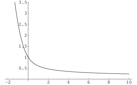
The plot of against for the branch of (6.73) is shown in figure 1, where we fixed . Note that there are two branches. On the left hand side, starts at (where the curvature singularity lies) when , and increases till it becomes infinite at . On the right hand side , asymptotic infinity is at and the radius decreases until a finite value at . For spherical or toroidal symmetry, , and , the left-hand branch has a conventional horizon at which vanishes, for a range of couplings although the right-hand one does not. When it is the right-hand branch that has a conventional horizon for a range of couplings, while the left-hand branch has .

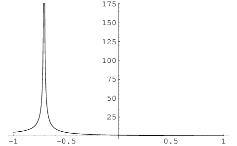
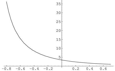
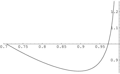
The branch of (6.73) is shown in figure 2 for the same values of the parameters. It is just the mirror image of the branch. For both signs of , although the solutions start at a minimum , the curvature is singular there ().
In figure 3 we plot as a function of for the solutions above. At the curvature singularity it is .
For large distances (which makes sense for ), the leading behavior of (6.73) for the solutions with positive mass is
| (6.75) |
with
| (6.76) |
Moreover we have
| (6.77) |
This implies that .
6.2
In this case, can have either sign and or .
The general solution for in this case is given implicitly as
| (6.78) |
where is a sign and is the integration constant. The modified lapse function is
| (6.79) |
where we have chosen the multiplicative integration constant so that the function asymptotes to one at infinite distance.
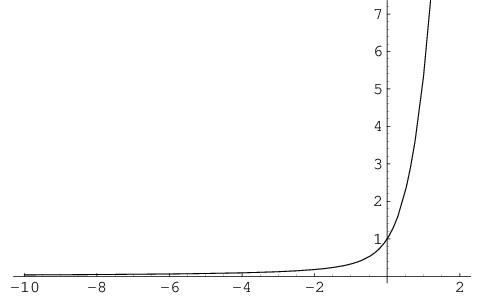
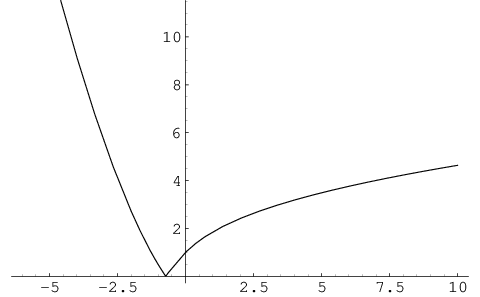
Plots of the solutions above for different values and signs of and are portrayed in figures 4 and 5. In this case, ranges from to infinity. There is also here a curvature singularity at .

For large distances , which for makes sense for , , while for , , , the leading behavior is achieved with the vanishing of the first factor in (6.78) and we obtain for the solutions with positive mass
| (6.80) |
| (6.81) |
| (6.82) |
Note that
to obtain the result (6.82) one has to consider in the
expansion of (6.80) also the exact term.
This implies that also here .
For , there is another way to make something vanish on the left-hand side of (6.78) and this is to have . This gives a different asymptotic behavior at large
| (6.83) |
Note than in this case the exponent is negative and spans all real negative values as . This is a case where the long distance behavior in the function is stronger than the generic AdS behavior.
6.3
The value is a special one for equation (6.72) with corresponding solution
| (6.84) |
where and are integration constants. Note that is allowed for the solution (6.78) but not for the solution (6.73).
Detailed-balance with arbitrary has
| (6.85) |
and therefore corresponds to this last case. Substituting these values for in (6.84) we obtain
| (6.86) |
which is the first solution found in [6] with generic .
When we choose further for the integration constant in (6.84) we find , and then, for detailed-balance with arbitrary , the lapse remains undetermined, which is the second solution found in [6] with generic .
We end by noting that in the generic case with the exception of , there are always solutions with the standard asymptotic behavior exemplified in (6.75), (6.77) (or the same (6.80), (6.82)). The solutions are generically asymptotically AdS/dS, with a standard tale that defines the mass of the solution. In all such cases the solutions come in a pair with different asymptotic effective cosmological constants
| (6.87) |
Not only the bare cosmological constant is responsible for but also the curvature square couplings . This is special example of what is known in cosmology as self-acceleration: the generation of acceleration (background curvature) by gravity alone.
The effective cosmological constant can become zero and the solution asymptotically flat when . In this case, the solution is asymptotically flat, while the solution has
| (6.88) |
7 The horizons in the generic case
We define again the exterior horizon position as the largest root of equation . This implies that
| (7.89) |
where we defined the variable that will be useful later on.
7.1
From (6.73) we obtain an equation for
| (7.90) |
The existence of the square root implies an upper bound on
| (7.91) |
For a flat horizon , the inequality constraints the couplings
| (7.92) |
7.2
From (6.78) we obtain an equation for
| (7.93) |
8 Thermodynamics in the generic case
We now investigate the relevant thermodynamics in the generic case following the remarks and assumptions of section 3.3.
8.1
As showed before, there are solutions with the standard asymptotic behavior (6.75),(6.77). For simplicity we assume that , so that .
We calculate the entropy by assuming the first law , from which
| (8.96) |
For , integration gives
| (8.97) |
where we have set so that .
For (where the inequality (7.91) is relevant)
| (8.98) |
where
| (8.99) |
while , h are used for , respectively.
8.2
Also here, there are solutions with the standard asymptotic behavior (6.80),(6.82). We will study the case with and for simplicity we assume that , so that .
The Hawking temperature in this case is computed to be
| (8.100) |
while the mass is
Using the first law, we calculate the entropy by integration as before. For , this integration gives again (8.97).
For , we obtain
where
| (8.102) |
We note that the expression () has a logarithmic divergence when for both branches , due to the first factor inside the logarithm.
9 Discussion and further directions
We have found the most general spherically symmetric solution to Hořava-Lifshitz type of gravity theories with zero shift. The action used was general except at the level cubic in curvatures where the Cotton2 combination was used. We do not expect new qualitatively different effects if we allow also the most general (curvature)3 couplings.
It is a generic feature of the solutions found that they have regular large distance asymptotics that are asymptotically AdS/dS or flat. Moreover, generically the next correction is compatible with a standard Newton’s law.
There are exceptions to this results that are special. In particular, the detailed balance action first written down by Horǎva is one of these notable exceptions. As shown already first in [6] it does not reproduce the correct Newton law at large distances. This is part of a class of special cases analyzed here, occurring when
| (9.103) |
although in the second case it is not the generic solution.
In one of the two general categories of parameters () where the horizon distance is permitted to shrink to zero, the entropy has a logarithmic divergence in this limit. In the other general category () the horizon distance is bounded from below.
For special values of the curvature-squared couplings , when the horizon position is allowed to go to zero the entropy is regular in this limit.
For the same values of the curvature-squared couplings , , there exists a solution with logarithmically corrected large distance asymptotics. Its “mass parameter” defined in the naive way, depends logarithmically on radial distance and becoming smaller at larger distances.
When the cosmological constant term in the action is absent, the effective cosmological constant of curvature is also zero (for some branches).
We have studied geodesics of particles with finite and infinite light speeds in spherically symmetric backgrounds with traditional horizons. We parameterize the dispersion relations of particles as , with . We find that when the traditional behavior of the horizon disappears suggesting that for such particles that black hole is effectively “naked”.
There are several interesting questions remaining open.
- •
The meaning of the notion of a black-hole and that of horizon in a theory with particles that have modified dispersion relations must be investigated. In particular, apparent puzzles/instabilities that seem to exist in such cases must be resolved or such theories will be physically discredited. A key element that may turn out to be important is a strong downgrading of energy in cases of modified dispersion relations that together with low energy Lorentz invariance may be a way to resolve puzzles.
- •
Finer properties of the black hole found should be studied as well as extremal limit in search for stronger constraints on the physical acceptability of such solutions
- •
Spherically symmetric solutions in the projectable theory need to be studied as no non-trivial one is known so far.
- •
The study of the non-linear structure of spherically symmetric solutions in the modified non-projectable theory of [23] must be studied in order to evaluate the stability claims of such solutions at the non-linear level.
We plan to return to these question in the near future.
Acknowledgements
We are grateful to C. Charmousis, R. Parentani and H. B. Zhang for valuable discussions.
This work was partially supported by a European Union grant FP7-REGPOT-2008-1-CreteHEP Cosmo-228644, and a CNRS PICS grant # 4172.
APPENDIX
Appendix A The classical equations of motion
We now add the action of matter
| (A.104) |
to the gravitational action (2.15) and we will vary with respect to the gravitational fields to obtain the equations of motion.
The equation obtained by varying N is
| (A.105) |
with
| (A.106) |
The equation obtained by varying is
| (A.107) |
Finally, the equation of motion obtained by varying is more voluminous
| (A.108) |
where was defined below equation (2.9), ; stands for covariant differentiation with respect to the metric , and
| (A.109) |
Appendix B Derivation of solution when , .
In this case, equation (3.24) becomes
| (B.110) |
We define a new function and a new coordinate
| (B.111) |
Equation (B.110) becomes
| (B.112) |
where a dot is a derivative with respect to .
The general solution of equation (B.112) must have , and has two branches with . It is given by the implicit expression
| (B.113) |
where is integration constant (positive or negative).
We proceed with the integration of equation (3.29) and define
| (B.114) |
where in the last equality we used equation (B.113).
Moreover, using (B.112), we obtain , and therefore
| (B.115) |
Equation (3.29) now becomes
| (B.116) |
Equation (B.116) can be integrated to
| (B.117) |
with integration constant. In terms of the variable it becomes,
| (B.118) |
where we fixed the integration constant .
Equation (B.118), together with (B.113) provide the general solution when . This solution can be given alternatively in terms of the variable as
| (B.119) |
| (B.120) |
Above, the branch with corresponds to , while corresponds to .
We will now study the large distance, behavior of the solutions above.
- •
For large distances , the branch of (B.113) can be approximated as , and therefore
(B.121) For an asymptotically AdS or flat solution we must therefore impose .
For the modified lapse and the lapse we obtain
(B.122) - •
In the case with , the large distance limit is achieved when . We find to leading order that
(B.123) Therefore, such terms logarithmically dominate the cosmological constant in the large distance limit.
Appendix C The general solution
In this appendix we describe first the general solution of equation (5.58) that we reproduce here for convenience.
| (C.128) |
We change variables as
| (C.129) |
with dot being the derivative with respect to . We also introduce
| (C.130) |
so that equation (C.128) is
| (C.131) |
From (C.132) we observe that . If satisfies the first order differential equation
| (C.133) |
then, is given as
| (C.134) |
This is the general solution for . This is shown by defining
| (C.135) |
and showing that equation (C.132) implies that satisfies equation (C.133), and is given by (C.134).
Since (C.134) gives , only will be determined from the solution, and therefore, two branches will always arise for each solution . From (C.134), we must have .
Equation (C.133) leads to a quadrature
| (C.136) |
where are integration constants. The integrant can be broken as
| (C.137) |
The integration of the first two terms in (C.137) gives
| (C.138) |
The integration of the third term depends on the sign of . There are two cases, one for and another for .
Before we proceed to consider the two cases, we should also consider the second equation, namely (3.29) that in terms of the current variables, its coefficients translate as
| (C.139) |
Therefore, equation (3.29) is rewritten as
| (C.140) |
We now consider the two cases separately.
C.1
Equation (C.130) implies that and a solution exists only for . The solution for is
| (C.141) |
and for we have the implicit equation
| (C.142) |
with taking both positive and negative values and .
Using , we may rewrite the solution (C.142) as an implicit equation for as
| (C.143) |
Integration of equation (C.140) gives
| (C.144) |
and using (C.141) we obtain
| (C.145) |
and in terms of
| (C.146) |
Finally, we choose for convenience the constant of integration as
| (C.147) |
so that the final solution becomes
| (C.148) |
For large distance (which makes sense for ), the leading behavior of (C.143) for the solutions with positive mass is
| (C.149) |
We therefore obtain
| (C.150) |
with
| (C.151) |
Moreover we have
| (C.152) |
To obtain the entropy expression (8.98) for it is helpful to convert to ,
| (C.153) |
where we can find
| (C.154) |
| (C.155) |
so finally,
| (C.156) |
This integration can be done explicitly in terms of defining and replacing in terms of .
C.2
In this case we have or . The solution from (C.136) is
| (C.157) |
and in terms of
| (C.158) |
where , is the integration constant, and
.
Finally, the solution (C.158) is written in terms of
as
| (C.159) |
where is allowed to take both positive and negative values.
Integration of equation (C.140) gives
| (C.160) |
and using (C.157) we obtain
| (C.161) |
which can be rewritten in terms of as
| (C.162) |
Choosing , we obtain
| (C.163) |
For large distance (for , or , ) the leading behavior of (C.159) for the solutions with positive mass is
| (C.164) |
We therefore obtain
| (C.165) |
Moreover we have
| (C.166) |
To obtain the entropy expression () for it is helpful to convert to ,
| (C.167) |
where we can find
| (C.168) |
| (C.169) |
so finally,
| (C.170) |
This integration can be done explicitly in terms of defining and replacing in terms of .
Appendix D Dispersive geodesics
Particles with non-standard dispersion relations, and in particular non-Lorentz invariant ones, do not follow the usual geodesics in the gravitational field. This has been discussed in several very recent works [26], [27], [28]. We will follow a slightly different approach here to study dispersive geodesics. We will eventually investigate the fate of the horizon for such particles and find that it seems to disappear, as intuition suggests.
To proceed, we write the metric in the ADM form
| (D.171) |
as well as the inverse metric
| (D.172) |
where indices of are raised with the spatial metric .
We will also consider a scalar mode which in the standard relativistic case has a coupling to gravity in ADM notation given by
| (D.173) |
For the non-relativistic case we write a general non-relativistic quadratic action in the Lifshitz spirit as
| (D.174) |
with equations of motion
| (D.175) |
where in the spatial part we neglected derivatives acting on as they will be irrelevant in the derivation of the geodesic (geometric optics) equations.
To pass to point-like trajectories, we replace , , and neglect metric derivatives to obtain the equivalent Hamiltonian (“zero energy”) constraint
| (D.176) |
This is implemented with a Lagrange multiplier , to obtain the world-line action as
| (D.177) |
where is the affine time of the path and dot stands for . is a one-dimensional einbein. The action (D.177) is invariant under general reparametrization of the affine time
| (D.178) |
Using such reparametrizations the einbein can be set to a constant .
The classical path equations come from varying , , and . The variation of by definition gives (D.176) while the momentum variations give
| (D.179) |
| (D.180) |
Finally the variations over the coordinates give
| (D.181) |
Equation (D.180) gives
| (D.182) |
This is a non-linear equation in general, and we can pick a solution . Then we can express
| (D.183) |
We also obtain by substitution
| (D.184) |
where in the last equation we used (D.182). We also have
| (D.185) |
and finally the on-shell action is
| (D.186) |
where should be thought as a function of the metric, , and the einbein as given from (D.182). Indeed varying using the constraint (2.5)gives that appropriate geodesic equations and the zero energy constraint. This action reduces to the standard relativistic action for .
We now consider a particle with a non-standard dispersion relation (corresponds to a dispersion relation ) a radial geodesic and a spherical symmetric BH metric to obtain
| (D.187) |
| (D.188) |
where is a constant of integration (energy).
From (D.172) we also obtain
| (D.189) |
For any the geodesic is regular at the zeros of .
If at has an a-th order zero and a b-th order zero, then the geodesic is singular if
| (D.190) |
We have always . In the case of HL we expect generically that , therefore the condition is . For a single zero of , and then that is unlikely. Generically .
For a double zero of , then we always have a singularity. This suggests that only extremal BH have a horizon in support of the intuitive notion that if a particle has a dispersion relation with an infinite speed of propagation, then it feels no horizon in the background of BH solutions.
References
- [1]
P. Hořava,
“Quantum Criticality and Yang-Mills Gauge Theory,”
[ArXiv:0811.2217][hep-th];
“Membranes at Quantum Criticality,” JHEP 0903 (2009) 020 [ArXiv:0812.4287][hep-th];
“Quantum Gravity at a Lifshitz Point,” [ArXiv:0901.3775][hep-th];
“Spectral Dimension of the Universe in Quantum Gravity at a Lifshitz Point,” [ArXiv:0902.3657][hep-th]. - [2] J. Kluson, “Branes at Quantum Criticality,” [ArXiv:0904.1343][hep-th].
- [3] E. Kiritsis and G. Kofinas, “Hořava-Lifshitz Cosmology,”, Nucl. Phys. B821 (2009) 467-480, [ArXiv:0904.1334][hep-th].
- [4]
T. P. Sotiriou, M. Visser and S. Weinfurtner,
“Phenomenologically viable Lorentz-violating quantum gravity,”
Phys. Rev. Lett. 102 (2009) 251601
[ArXiv:0904.4464][hep-th];
“Quantum gravity without Lorentz invariance,” [ArXiv:0905.2798][hep-th]. - [5] H. Nastase, “On IR solutions in Horava gravity theories,” [ArXiv:0904.3604][hep-th].
- [6] H. Lu, J. Mei and C. N. Pope, “Solutions to Horava Gravity,” [ArXiv:0904.1595][hep-th].
- [7] E. Kiritsis, “Holography and brane-bulk energy exchange,” JCAP 0510 (2005) 014 [ArXiv:hep-th/0504219].
- [8] S. Mukohyama, “Scale-invariant cosmological perturbations from Horava-Lifshitz gravity without inflation,” JCAP 0906 (2009) 001 [ArXiv:0904.2190][hep-th].
- [9] G. Calcagni, “Cosmology of the Lifshitz universe,” [ArXiv:0904.0829][hep-th].
- [10] R. Brandenberger, “Matter Bounce in Horava-Lifshitz Cosmology,” [ArXiv:0904.2835][hep-th].
- [11] T. Takahashi and J. Soda, “Chiral Primordial Gravitational Waves from a Lifshitz Point,” Phys. Rev. Lett. 102, 231301 (2009) [ArXiv:0904.0554][hep-th].
- [12] S. Mukohyama, “Dark matter as integration constant in Horava-Lifshitz gravity,” [ArXiv:0905.3563][hep-th].
- [13]
Y. S. Piao,
“Primordial Perturbation in Horava-Lifshitz Cosmology,”
[ArXiv:0904.4117][hep-th];
X. Gao, “Cosmological Perturbations and Non-Gaussianities in Hořava-Lifshitz Gravity,” [ArXiv:0904.4187][hep-th];
S. Mukohyama, K. Nakayama, F. Takahashi and S. Yokoyama, “Phenomenological Aspects of Horava-Lifshitz Cosmology,” [ArXiv:0905.0055][hep-th];
T. Ha, Y. Huang, Q. Ma, K. D. Pechan, T. J. Renner, Z. Wu and A. Wang, “Classification of the FRW universe with a cosmological constant and a perfect fluid of the equation of state ,” [ArXiv:0905.0396][physics.pop-ph];
B. Chen, S. Pi and J. Z. Tang, “Scale Invariant Power Spectrum in Hořava-Lifshitz Cosmology without Matter,” [ArXiv:0905.2300][hep-th];
E. N. Saridakis, “Horava-Lifshitz Dark Energy,” [ArXiv:0905.3532][hep-th];
X. Gao, Y. Wang, R. Brandenberger and A. Riotto, “Cosmological Perturbations in Hořava-Lifshitz Gravity,” [ArXiv:0905.3821][hep-th];
A. Wang and Y. Wu, “Thermodynamics and classification of cosmological models in the Horava-Lifshitz theory of gravity,” JCAP 0907 (2009) 012 [ArXiv:0905.4117][hep-th];
S. Nojiri and S. D. Odintsov, “Covariant Horava-like renormalizable gravity and its FRW cosmology,” [ArXiv:0905.4213][hep-th];
Y. F. Cai and E. N. Saridakis, “Non-singular cosmology in a model of non-relativistic gravity,” [ArXiv:0906.1789][hep-th];
Y. F. Cai and X. Zhang, “Primordial perturbation with a modified dispersion relation,” [ArXiv:0906.3341][astro-ph.CO];
K. Yamamoto, T. Kobayashi and G. Nakamura, “Breaking the scale invariance of the primordial power spectrum in Horava-Lifshitz Cosmology,” [ArXiv:0907.1549][astro-ph.CO];
A. Wang and R. Maartens, “Linear perturbations of cosmological models in the Horava-Lifshitz theory of gravity without detailed balance,” [ArXiv:0907.1748][hep-th];
M. R. Setare, “Interacting Dark Energy in Hořava-Lifshitz Cosmology,” [ArXiv:0909.0456][hep-th];
T. Kobayashi, Y. Urakawa and M. Yamaguchi, “Large scale evolution of the curvature perturbation in Horava-Lifshitz cosmology,” [ArXiv:0908.1005][astro-ph.CO];
S. Maeda, S. Mukohyama and T. Shiromizu, “Primordial magnetic field from non-inflationary cosmic expansion in Horava-Lifshitz gravity,” [ArXiv:0909.2149][astro-ph.CO];
S. Carloni, E. Elizalde and P. J. Silva, “An analysis of the phase space of Horava-Lifshitz cosmologies,” [ArXiv:0909.2219][hep-th];
G. Leon and E. N. Saridakis, “Phase-space analysis of Horava-Lifshitz cosmology,” [ArXiv:0909.3571][Unknown];
A. Wang, D. Wands and R. Maartens, “Scalar field perturbations in Horava-Lifshitz cosmology,” [ArXiv:0909.5167][Unknown]. - [14] A. Kehagias and K. Sfetsos, “The black hole and FRW geometries of non-relativistic gravity,” Phys. Lett. B 678 (2009) 123 [ArXiv:0905.0477][hep-th].
- [15] M. I. Park, “The Black Hole and Cosmological Solutions in IR modified Horava Gravity,” [ArXiv:0905.4480][hep-th].
- [16]
R. G. Cai, L. M. Cao and N. Ohta,
“Topological Black Holes in Horava-Lifshitz Gravity,”
[ArXiv:0904.3670][hep-th]; Y. S. Myung and Y. W. Kim,
“Thermodynamics of Hořava-Lifshitz black holes,”
[ArXiv:0905.0179][hep-th];
R. G. Cai, L. M. Cao and N. Ohta, “Thermodynamics of Black Holes in Horava-Lifshitz Gravity,” [ArXiv:0905.0751][hep-th];
A. Ghodsi, “Toroidal solutions in Horava Gravity,” [ArXiv:0905.0836][hep-th];
Y. S. Myung, “Thermodynamics of black holes in the deformed Hořava-Lifshitz gravity,” Phys. Lett. B 678 (2009) 127 [ArXiv:0905.0957][hep-th];
S. b. Chen and J. l. Jing, “Strong field gravitational lensing in the deformed Hǒrava-Lifshitz black hole,” [ArXiv:0905.2055][gr-qc];
A. Ghodsi and E. Hatefi, “Extremal rotating solutions in Horava Gravity,” [ArXiv:0906.1237][hep-th];
H. W. Lee, Y. W. Kim and Y. S. Myung, “Extremal black holes in the Hořava-Lifshitz gravity,” [ArXiv:0907.3568][hep-th];
Y. S. Myung, “Entropy of black holes in the deformed Hořava-Lifshitz gravity,” [ArXiv:0908.4132][hep-th]. - [17] R. G. Cai, B. Hu and H. B. Zhang, “Dynamical Scalar Degree of Freedom in Horava-Lifshitz Gravity,” [ArXiv:0905.0255][hep-th].
- [18] C. Charmousis, G. Niz, A. Padilla and P. M. Saffin, [ArXiv:0905.2579][hep-th].
- [19] Y. W. Kim, H. W. Lee and Y. S. Myung, “Nonpropagation of scalar in the deformed Hořava-Lifshitz gravity,” [ArXiv:0905.3423][hep-th].
- [20] D. Blas, O. Pujolas and S. Sibiryakov, “On the Extra Mode and Inconsistency of Horava Gravity,” [ArXiv:0906.3046][hep-th].
- [21] S. Mukohyama, “Caustic avoidance in Horava-Lifshitz gravity,” [ArXiv:0906.5069][hep-th].
- [22] C. Bogdanos and E. N. Saridakis, “Perturbative instabilities in Horava gravity,” [ArXiv:0907.1636][hep-th].
- [23] D. Blas, O. Pujolas and S. Sibiryakov, “A healthy extension of Horava gravity,” [ArXiv:0909.3525][hep-th].
- [24]
R. A. Konoplya,
“Towards constraining of the Horava-Lifshitz gravities,”
[ArXiv:0905.1523][hep-th];
T. Harko, Z. Kovacs and F. S. N. Lobo, “Testing Hořava-Lifshitz gravity using thin accretion disk properties,” [ArXiv:0907.1449][gr-qc];
S. S. Kim, T. Kim and Y. Kim, “Surplus Solid Angle: Toward Astrophysical Test of Horava-Lifshitz Gravity,” [ArXiv:0907.3093][hep-th];
T. Harko, Z. Kovacs and F. S. N. Lobo, “Solar system tests of Hořava-Lifshitz gravity,” [ArXiv:0908.2874][gr-qc]. - [25]
B. Chen and Q. G. Huang,
“Field Theory at a Lifshitz Point,”
[ArXiv:0904.4565][hep-th];
D. Orlando and S. Reffert, “On the Renormalizability of Horava-Lifshitz-type Gravities,” Class. Quant. Grav. 26 (2009) 155021 [ArXiv:0905.0301][hep-th];
J. Kluson, “Horava-Lifshitz f(R) Gravity,” [ArXiv:0907.3566][hep-th];
S. K. Chakrabarti, E. N. Saridakis and A. A. Sen, “A new approach to modified-gravity models,” [ArXiv:0908.0293][astro-ph.CO];
- [26] D. Capasso and A. P. Polychronakos, “Particle Kinematics in Horava-Lifshitz Gravity,” [ArXiv:0909.5405][Unknown].
- [27] T. Suyama, “Notes on Matter in Horava-Lifshitz Gravity,” [ArXiv:0909.4833][Unknown].
- [28] S. K. Rama, “Particle Motion with Hořava – Lifshitz type Dispersion Relations,” [ArXiv:0910.0411][hep-th].
- [29] D. Mattingly, “Modern tests of Lorentz invariance,” Living Rev. Rel. 8 (2005) 5 [ArXiv:gr-qc/0502097].
- [30] V. A. Kostelecky and N. Russell, “Data Tables for Lorentz and CPT Violation,” [ArXiv:0801.0287][hep-ph].
- [31]
M. Galaverni and G. Sigl,
“Lorentz Violation and Ultrahigh-Energy Photons,”
Phys. Rev. D 78 (2008) 063003
[ArXiv:0807.1210][astro-ph];
J. W. Elliott, G. D. Moore and H. Stoica, “Constraining the new aether: Gravitational Cherenkov radiation,” JHEP 0508 (2005) 066 [ArXiv:hep-ph/0505211]. - [32] S. Liberati and L. Maccione, “Lorentz Violation: Motivation and new constraints,” [ArXiv:0906.0681][astro-ph.HE].
- [33]
D. Anselmi and M. Halat,
“Renormalization of Lorentz violating theories,”
Phys. Rev. D 76 (2007) 125011
[ArXiv:0707.2480][hep-th];
“Weighted power counting and Lorentz violating gauge theories. I: General properties,” Annals Phys. 324 (2009) 874 [ArXiv:0808.3470][hep-th];
“Weighted power counting and Lorentz violating gauge theories. II: Classification,” Annals Phys. 324 (2009) 1058 [ArXiv:0808.3474][hep-th]. - [34] “Standard Model Without Elementary Scalars And High Energy Lorentz Violation,” [ArXiv:0904.1849][hep-ph].
- [35]
S. Corley and T. Jacobson,
“Hawking Spectrum and High Frequency Dispersion,”
Phys. Rev. D 54 (1996) 1568
[ArXiv:hep-th/9601073];
“Black hole lasers,” Phys. Rev. D 59 (1999) 124011 [ArXiv:hep-th/9806203]. - [36] J. Macher and R. Parentani, “Black/White hole radiation from dispersive theories,” Phys. Rev. D 79 (2009) 124008 [ArXiv:0903.2224][hep-th].
- [37]
S. L. Dubovsky and S. M. Sibiryakov,
“Spontaneous breaking of Lorentz invariance, black holes and perpetuum
mobile of the 2nd kind,”
Phys. Lett. B 638 (2006) 509
[ArXiv:hep-th/0603158];
C. Eling, B. Z. Foster, T. Jacobson and A. C. Wall, “Lorentz violation and perpetual motion,” Phys. Rev. D 75 (2007) 101502 [ArXiv:hep-th/0702124];
E. Kant, F. R. Klinkhamer and M. Schreck, “Lorentz violation and black-hole thermodynamics: Compton scattering process,” [ArXiv:0909.0160][hep-th]. - [38] R. G. Cai and N. Ohta, “Horizon Thermodynamics and Gravitational Field Equations in Horava-Lifshitz Gravity,” [ArXiv:0910.2307][hep-th].
- [39] R. M. Wald, “Black hole entropy is the Noether charge,” Phys. Rev. D 48 (1993) 3427 [ArXiv:gr-qc/9307038].