Smoothness of Gaussian conditional independence modelsThanks: This material is based upon work supported by the National Science Foundation under Grant No. DMS-0746265. Mathias Drton was also supported by an Alfred P. Sloan Fellowship.

Mathias Drton Address: Department of Statistics, 5734 S. University Ave, Chicago, IL 60637 Email address: drton@uchicago.edu and Han Xiao Address: Department of Statistics, 5734 S. University Ave, Chicago, IL 60637 Email address: xiao@galton.uchicago.edu

Abstract.

Conditional independence in a multivariate normal (or Gaussian) distribution is characterized by the vanishing of subdeterminants of the distribution’s covariance matrix. Gaussian conditional independence models thus correspond to algebraic subsets of the cone of positive definite matrices. For statistical inference in such models it is important to know whether or not the model contains singularities. We study this issue in models involving up to four random variables. In particular, we give examples of conditional independence relations which, despite being probabilistically representable, yield models that non-trivially decompose into a finite union of several smooth submodels.

2000 Mathematics Subject Classification

Primary 62H05

1. Introduction

Conditional independence (CI) is one of the most important notions of multivariate statistical modelling. Many popular statistical models can be thought of as being defined in terms of CI constraints. For instance, the popular graphical models are obtained by identifying a considered set of random variables with the nodes of a graph and converting separation relations in the graph into CI statements [Lau96]. Despite the use of different graphs and separation criteria, graphical models present only a small subset of the models that can be defined using conditional independence [Stu05]. It is thus of interest to explore to which extent more general collections of CI constraints may furnish other well-behaved statistical models. In this paper we pursue this problem under the assumption that the considered random vector is Gaussian, that is, it has a joint multivariate normal distribution. A precise formulation of the problem is given in Question 1.1 below.

Let $X=(X_{1},\dots,X_{m})$ be a Gaussian random vector with mean vector $\mu$ and covariance matrix $\Sigma$ , in symbols, $X\sim\mathcal{N}_{m}(\mu,\Sigma)$ . All covariance matrices appearing in this paper are tacitly assumed positive definite, in which case $X$ is also referred to as regular Gaussian. We denote the subvector given by an index set $A\subseteq[m]:=\{1,\dots,m\}$ by $X_{A}$ . For three pairwise disjoint index sets $A,B,C\subseteq[m]$ , we write $A\mbox{$\perp\kern-5.5pt\perp$}B\,|\,C$ to abbreviate the conditional independence of $X_{A}$ and $X_{B}$ given $X_{C}$ . We use concatenation of symbols to denote unions of index sets, that is, $AB=A\cup B$ , and make no distinction between indices and singleton index sets such that $i=\{i\}$ and $ij=\{i,j\}$ . A general introduction to conditional independence can be found in [Stu05], but since this paper is solely concerned with the Gaussian case the reader may also simply treat the following proposition as a definition. It states that conditional independence in a Gaussian random vector is an algebraic constraint on its covariance matrix. For a proof see for example [DSS09, §3.1].

Proposition 1.1.

Let $X\sim\mathcal{N}_{m}(\mu,\Sigma)$ be a (regular) Gaussian random vector and $A,B,C\subset[m]$ pairwise disjoint index sets. Then $A\mbox{$\perp\kern-5.5pt\perp$}B\,|\,C$ if and only if the submatrix $\Sigma_{AC,BC}$ has rank equal to the cardinality of $C$ . Moreover, $A\mbox{$\perp\kern-5.5pt\perp$}B\,|\,C$ if and only if $i\mbox{$\perp\kern-5.5pt\perp$}j\,|\,C$ for all $i\in A$ and $j\in B$ .

The proposition clarifies in particular that one may restrict attention to pairwise statements $i\mbox{$\perp\kern-5.5pt\perp$}j\,|\,C$ . We remark that this is also true for arbitrary (non-Gaussian) random vectors as it can still be shown that $A\mbox{$\perp\kern-5.5pt\perp$}B\,|\,C$ if and only if

i\mbox{$\perp\kern-5.5pt\perp$}j\,|\,D\quad\text{for all}\quad i\in A,\>j\in B,\>C\subseteq D\subseteq ABC\setminus ij;

see [Mat92, Lemma 3]. Since $i\mbox{$\perp\kern-5.5pt\perp$}j\,|\,C$ if and only if $j\mbox{$\perp\kern-5.5pt\perp$}i\,|\,C$ , pairwise statements can also be represented using an index set couple $ij|C$ that groups a two-element set $ij\subseteq[m]$ and a conditioning set $C\subseteq[m]\setminus ij$ . Following [LM07] we refer to these couples as conditional independence couples.

A conditional independence relation is a set of CI couples. We write $\mathcal{R}(m)$ for the maximal relation comprising all $\binom{m}{2}\cdot 2^{m-2}$ CI couples over the set $[m]$ . A CI relation $\mathcal{L}\subseteq\mathcal{R}(m)$ determines a Gaussian conditional independence model, namely, the family of all multivariate normal distributions for which $i\mbox{$\perp\kern-5.5pt\perp$}j\,|\,C$ whenever $ij|C\in\mathcal{L}$ . Since conditional independence constrains only the covariance matrix of a Gaussian random vector, the Gaussian model given by $\mathcal{L}$ corresponds to the algebraic subset

(1.1)

V_{\mathit{pd}}(\mathcal{L})=\big\{\,\Sigma\in\mathit{PD}_{m}\>:\>\det(\Sigma_{iC,jC})=0\;\text{for all}\;ij|C\in\mathcal{L}\,\big\}

of the cone of positive definite $m\times m$ -matrices, here denoted by $\mathit{PD}_{m}$ .

Standard large-sample asymptotic methodology can be applied for statistical inference in a Gaussian CI model if $V_{\mathit{pd}}(\mathcal{L})$ is a smooth manifold. However, such techniques may fail under the presence of singularities [Drt09], which leads to the following natural question:

Question 1.1.

For which conditional independence relations $\mathcal{L}\subseteq\mathcal{R}(m)$ is the associated set $V_{\mathit{pd}}(\mathcal{L})$ a smooth manifold?

If $m=2$ the question is trivial because the set $V_{\mathit{pd}}(\mathcal{L})$ is either the positive definite cone or the set of diagonal $2\times 2$ -matrices. For $m=3$ , smoothness can fail in precisely one well-known way; compare (2.11) and Proposition 4.2 below.

Proposition 1.2.

For $m=3$ , the sets $V_{\mathit{pd}}(\mathcal{L})$ are smooth manifolds unless the conditional independence relation $\mathcal{L}$ is equal to $\{ij,\,ij|k\}$ for distinct indices $i,j,k$ .

In this paper we will answer the question for $m=4$ . Note that there are $2^{24}=16,777,216$ relations on $[m]=[4]$ . However, two relations may induce the same Gaussian model. For instance, $V_{\mathit{pd}}(\mathcal{L})=V_{\mathit{pd}}(\mathcal{K})$ for $\mathcal{L}=\{12,13|2\}$ and $\mathcal{K}=\{12,13,12|3,13|2\}$ . Therefore, we begin our study of Question 1.1, by finding all Gaussian CI models for a random vector of length $m=4$ . In this work we build heavily on the work [LM07] that determines the CI relations that are representable in Gaussian random vector of length $m\leq 4$ ; see also [Šim06a, Šim06b].

Definition 1.1.

A relation $\mathcal{L}$ is representable if there exists a covariance matrix $\Sigma\in\mathit{PD}_{m}$ for which $\det(\Sigma_{iC,jC})=0$ if and only if $ij|C\in\mathcal{L}$ .

The remainder of this paper is structured as follows. All Gaussian CI models for $m=4$ random variables are found in Section 2. Correlation matrices and helpful methods from computational algebra are introduced in Section 3 and used to answer Question 1.1 for $m=4$ in Section 4. The findings are discussed in Section 5. Appendix A lists all Gaussian CI models and implications for $m=4$ .

2. Gaussian conditional independence models

As mentioned in the introduction, there is a many-to-one relationship between the relations $\mathcal{L}$ and the sets of covariance matrices $V_{\mathit{pd}}(\mathcal{L})$ . In this section we explore this relationship and determine all Gaussian CI models on four variables.

2.1. Complete relations and representable decomposition

Given a set of covariance matrices $W\subset\mathit{PD}_{m}$ , we can define a relation as

\mathcal{L}(W)=\big\{\,ij|C\in\mathcal{R}(m)\>:\>\det(\Sigma_{iC,jC})=0\;\text{for all}\;\Sigma\in W\,\big\}.

The operator $\mathcal{L}(\cdot)$ and the operator $V_{\mathit{pd}}(\cdot)$ , defined in Section 1, are both inclusion-reversing. In other words, if two relations satisfy $\mathcal{L}\subseteq\mathcal{K}$ then $V_{\mathit{pd}}(\mathcal{L})\supseteq V_{\mathit{pd}}(\mathcal{K})$ , and if two sets are ordered by inclusion as $V\subseteq W$ then $\mathcal{L}(V)\supseteq\mathcal{L}(W)$ . For any relation $\mathcal{L}$ , it holds that $\mathcal{L}\subseteq\mathcal{L}(V_{\mathit{pd}}(\mathcal{L}))$ .

Definition 2.1.

A relation $\mathcal{L}$ is complete if $\mathcal{L}=\mathcal{L}(V_{\mathit{pd}}(\mathcal{L}))$ , that is, if for every couple $ij|C\not\in\mathcal{L}$ there exists a covariance matrix $\Sigma\in V_{\mathit{pd}}(\mathcal{L})$ with $\det(\Sigma_{iC,jC})\not=0$ .

Clearly, there is a 1:1 correspondence between models and complete relations. The following result provides a useful decomposition into representable pieces.

Theorem 2.1.

Every conditional independence model $V_{\mathit{pd}}(\mathcal{L})$ has a representable decomposition, that is, it can be decomposed as

V_{\mathit{pd}}(\mathcal{L})=V_{\mathit{pd}}(\mathcal{L}_{1})\cup\dots\cup V_{\mathit{pd}}(\mathcal{L}_{k}),

where $\mathcal{L}_{1},\dots,\mathcal{L}_{k}$ are representable relations. The decomposition can be chosen minimal (i.e., $\mathcal{L}_{i}\not\subseteq\mathcal{L}_{j}$ for all $i\not=j$ ), in which case the relations $\mathcal{L}_{1},\dots,\mathcal{L}_{k}$ are unique up to reordering.

Proof.

Suppose not all models have a representable decomposition. Choose $V_{\mathit{pd}}(\mathcal{L})$ to be a model that is inclusion-minimal among those without a representable decomposition. Enlarging the relation if necessary, we may assume that $\mathcal{L}$ is complete. Since $\mathcal{L}$ cannot be representable, every matrix $\Sigma\in V_{\mathit{pd}}(\mathcal{L})$ is in $V_{\mathit{pd}}(\mathcal{L}\cup\{ij|C\})$ for some CI couple $ij|C\not\in\mathcal{L}$ . Therefore, there exist complete relations $\mathcal{K}_{1},\dots,\mathcal{K}_{l}$ , all proper supersets of $\mathcal{L}$ , such that

V_{\mathit{pd}}(\mathcal{L})=V_{\mathit{pd}}(\mathcal{K}_{1})\cup\dots\cup V_{\mathit{pd}}(\mathcal{K}_{l}).

The relation $\mathcal{L}$ being complete, each $V_{\mathit{pd}}(\mathcal{K}_{j})$ is a proper subset of $V_{\mathit{pd}}(\mathcal{L})$ . By the inclusion-minimal choice of $V_{\mathit{pd}}(\mathcal{L})$ , each $V_{\mathit{pd}}(\mathcal{K}_{j})$ has a representable decomposition. This, however, yields a contradiction as combining the decompositions of the $V_{\mathit{pd}}(\mathcal{K}_{j})$ provides a representable decomposition of $V_{\mathit{pd}}(\mathcal{L})$ .

A representable decomposition can be chosen to be minimal by removing unnecessary components. To show uniqueness, suppose that there are two distinct minimal representable decompositions

(2.1)	$\displaystyle V_{\mathit{pd}}(\mathcal{L})$	$\displaystyle=V_{\mathit{pd}}(\mathcal{L}_{1})\cup\dots\cup V_{\mathit{pd}}(\mathcal{L}_{k})$
and
(2.2)	$\displaystyle V_{\mathit{pd}}(\mathcal{L})$	$\displaystyle=V_{\mathit{pd}}(\mathcal{K}_{1})\cup\dots\cup V_{\mathit{pd}}(\mathcal{K}_{l}).$

Then, for each $i\in[k]$ , we have

V_{\mathit{pd}}(\mathcal{L}_{i})\;=\;V_{\mathit{pd}}(\mathcal{L}_{i})\cap V_{\mathit{pd}}(\mathcal{L})\;=\;\bigcup_{j=1}^{l}\left[\,V_{\mathit{pd}}(\mathcal{L}_{i})\cap V_{\mathit{pd}}(\mathcal{K}_{j})\,\right].

Since $V_{\mathit{pd}}(\mathcal{L}_{i})\cap V_{\mathit{pd}}(\mathcal{K}_{j})=V_{\mathit{pd}}(\mathcal{L}_{i}\cup\mathcal{K}_{j})$ and $\mathcal{L}_{i}$ is representable, it follows that $\mathcal{L}_{i}=\mathcal{L}_{i}\cup\mathcal{K}_{j}$ for some $j$ , which implies that $\mathcal{K}_{j}\subseteq\mathcal{L}_{i}$ . Applying the same argument with the role of the two decompositions reversed, we obtain that $\mathcal{L}_{s}\subseteq\mathcal{K}_{j}\subseteq\mathcal{L}_{i}$ . By minimality, $s=i$ , and thus, $\mathcal{L}_{i}=\mathcal{K}_{j}$ . Hence, every $\mathcal{L}_{i}$ appears in (2.2). It follows that $k\leq l$ . Reversing again the role of the decomposition, we find that $k=l$ and the $\mathcal{K}_{j}$ are just a permutation of the $\mathcal{L}_{i}$ . ∎

Theorem 2.2.

A relation $\mathcal{L}$ is complete if and only if it is an intersection of representable relations. The representable relations can be chosen to yield a representable decomposition of the model $V_{\mathit{pd}}(\mathcal{L})$ .

Proof.

Suppose a relation $\mathcal{L}$ is the intersection of representable relations $\mathcal{L}_{1},\dots,\mathcal{L}_{k}$ . Consider a CI couple $ij|C\in\mathcal{L}(V_{\mathit{pd}}(\mathcal{L}))$ , that is, $ij|C$ holds for all covariance matrices in $V_{\mathit{pd}}(\mathcal{L})$ . By assumption, $\mathcal{L}\subseteq\mathcal{L}_{i}$ for all $i\in[k]$ . Hence, $V_{\mathit{pd}}(\mathcal{L}_{i})\subseteq V_{\mathit{pd}}(\mathcal{L})$ and thus $ij|C\in\mathcal{L}(V_{\mathit{pd}}(\mathcal{L}_{i}))$ for all $i\in[k]$ . But $\mathcal{L}(V_{\mathit{pd}}(\mathcal{L}_{i}))=\mathcal{L}_{i}$ because the representable relations $\mathcal{L}_{i}$ are in particular complete. It follows that $ij|C$ is in each relation $\mathcal{L}_{1},\dots,\mathcal{L}_{k}$ and thus also in $\mathcal{L}$ .

Conversely, let $\mathcal{L}$ be a complete relation. Let $\mathcal{L}_{1},\dots,\mathcal{L}_{k}$ be representable relations that yield a representable decomposition of $V_{\mathit{pd}}(\mathcal{L})$ as in Theorem 2.1. Since $V_{\mathit{pd}}(\mathcal{L}_{i})\subseteq V_{\mathit{pd}}(\mathcal{L})$ for each $i\in[k]$ , we have that

\mathcal{L}\;=\;\mathcal{L}(V_{\mathit{pd}}(\mathcal{L}))\;\subseteq\;\mathcal{L}(V_{\mathit{pd}}(\mathcal{L}_{i}))\;=\;\mathcal{L}_{i}.

Hence, $\mathcal{L}$ is a subset of the intersection of $\mathcal{L}_{1},\dots,\mathcal{L}_{k}$ . Since we may deduce from

V_{\mathit{pd}}(\mathcal{L})\;=\;\bigcup_{i=1}^{k}V_{\mathit{pd}}(\mathcal{L}_{i})\;\subseteq\;V_{\mathit{pd}}\left(\bigcap_{i=1}^{k}\mathcal{L}_{i}\right)

that

\bigcap_{i=1}^{k}\mathcal{L}_{i}\;\subseteq\;\mathcal{L}\left(V_{\mathit{pd}}\left(\bigcap_{i=1}^{k}\mathcal{L}_{i}\right)\right)\;\subseteq\;\mathcal{L}(V_{\mathit{pd}}(\mathcal{L}))\;=\;\mathcal{L},

we have shown that $\mathcal{L}$ is the intersection of $\mathcal{L}_{1},\dots,\mathcal{L}_{k}$ . ∎

Example 2.1.

The following relations are derived from the marginal independence statements $1\mbox{$\perp\kern-5.5pt\perp$}23$ , $2\mbox{$\perp\kern-5.5pt\perp$}13$ and $1\mbox{$\perp\kern-5.5pt\perp$}234$ , respectively:

	$\displaystyle\mathcal{L}_{1}$	$\displaystyle=\{12,13,12\|3,13\|2\},$
	$\displaystyle\mathcal{L}_{2}$	$\displaystyle=\{12,23,12\|3,23\|1\},$
	$\displaystyle\mathcal{L}_{3}$	$\displaystyle=\{12,13,14,12\|3,12\|4,13\|2,13\|4,14\|2,14\|3,12\|34,13\|24,14\|23\}.$

All three are representable. Since $\mathcal{L}_{2}\cap\mathcal{L}_{3}$ is equal to $\mathcal{L}=\{12,12|3\}$ , the latter is a complete relation. However, $\mathcal{L}_{2}$ and $\mathcal{L}_{3}$ do not yield a representable decomposition of $V_{\mathit{pd}}(\mathcal{L})$ because

V_{\mathit{pd}}(\mathcal{L}_{2})\cup V_{\mathit{pd}}(\mathcal{L}_{3})\;\subsetneq\;V_{\mathit{pd}}(\mathcal{L}).

The minimal representable decomposition of $V_{\mathit{pd}}(\mathcal{L})$ is instead given by $\mathcal{L}_{1}$ and $\mathcal{L}_{2}$ .

Remark 2.1.

The graphical modelling literature also discusses strong completeness; see e.g. [LPM01]. A representable relation $\mathcal{L}$ is strongly complete if the covariance matrices $\Sigma\in V_{\mathit{pd}}(\mathcal{L})$ with $\mathcal{L}\not=\mathcal{L}(\{\Sigma\})$ form a lower-dimensional subset of $V_{\mathit{pd}}(\mathcal{L})$ . For the CI relations appearing in graphical modelling, the set $V_{\mathit{pd}}(\mathcal{L})$ typically possesses a polynomial parametrization. It follows that $V_{\mathit{pd}}(\mathcal{L})$ is the intersection of an irreducible algebraic variety and the cone $\mathit{PD}_{m}$ . Completeness then implies strong completeness by general results from algebraic geometry [CLO07].

2.2. All models on four variables

Call two relations $\mathcal{L}_{1}$ and $\mathcal{L}_{2}$ equivalent, if there exists a permutation of the indices in the ground set $[m]$ that turns $\mathcal{L}_{1}$ into $\mathcal{L}_{2}$ . In [LM07] it is shown that for $m=4$ , there are 53 equivalence classes of representable relations. In this section, we find all Gaussian conditional independence models for $m=4$ random variables by constructing all complete relations. The work in this section will lead to the proof of the following result:

Theorem 2.3.

There are 101 equivalence classes of complete relations on the set $[m]=[4]$ .

In the introduction, we stated the equality $V_{\mathit{pd}}(\mathcal{L})=V_{\mathit{pd}}(\mathcal{K})$ for the relations $\mathcal{L}=\{12,13|2\}$ and $\mathcal{K}=\{12,13,12|3,13|2\}$ as an example of two relations inducing the same model. Alternatively, we may view this as $\{12,13|2\}$ implying $\{12|3,13\}$ .

Definition 2.2.

A (Gaussian) conditional independence implication is an ordered pair of disjoint CI relations $(\mathcal{L}_{1},\mathcal{L}_{2})$ such that $V_{\mathit{pd}}(\mathcal{L}_{1})=V_{\mathit{pd}}(\mathcal{L}_{1}\cup\mathcal{L}_{2})$ . We denote the implication as $\mathcal{L}_{1}\Rightarrow\mathcal{L}_{2}$ and say that a relation $\mathcal{L}$ satisfies $\mathcal{L}_{1}\Rightarrow\mathcal{L}_{2}$ , if $\mathcal{L}_{1}\subseteq\mathcal{L}$ implies that $\mathcal{L}_{2}\subseteq\mathcal{L}$ .

Example 2.2.

Let $i,j,k\in[m]$ be distinct indices and $C\subset[m]\setminus ijk$ . Then the following are Gaussian CI implications:

(2.3)	$\displaystyle\{ij\|C,ik\|C\}$	$\displaystyle\Longrightarrow$	$\displaystyle\{ij\|kC,ik\|jC\}$
(2.4)	$\displaystyle\{ij\|C,ik\|jC\}$	$\displaystyle\Longrightarrow$	$\displaystyle\{ik\|C,ij\|kC\}$
(2.5)	$\displaystyle\{ij\|kC,ik\|jC\}$	$\displaystyle\Longrightarrow$	$\displaystyle\{ij\|C,ik\|C\}.$

Implication (2.3) follows from the last assertion in Proposition 1.1 and an implication known as weak union that holds for all probability distributions. Implication (2.4) is referred to as contraction and also holds for all probability distributions. The last implication, (2.5), is known as intersection and holds for many but not all non-Gaussian distributions. See for instance [DSS09, §3.1] for more background.

We now describe how to construct all complete relations by adapting the approach taken in the construction of all representable relations in [LM07]. A key concept is the following notion of duality.

Definition 2.3.

The dual of a couple $ij|C\in\mathcal{R}(m)$ is the couple $ij|\bar{C}$ where $\bar{C}=[m]\setminus ijC$ . The dual of a relation $\mathcal{L}$ on $[m]$ is the relation

\mathcal{L}^{d}=\{ij|\bar{C}\;:\;ij|C\in\mathcal{L}\}

made up of the dual couples of the elements of $\mathcal{L}$ .

Lemma 2.1.

For a positive definite matrix $\Sigma$ and two relations $\mathcal{L}$ and $\mathcal{K}$ :

(i)

$\mathcal{L}(\{\Sigma\})^{d}=\mathcal{L}(\{\Sigma^{-1}\})$ ;
(ii)

$\mathcal{L}\Rightarrow\mathcal{K}$ if and only if $\mathcal{L}^{d}\Rightarrow\mathcal{K}^{d}$ ;
(iii)

$\mathcal{L}$ is complete if and only if $\mathcal{L}^{d}$ has this property.

Proof.

(ii) and (iii) follow readily from (i), which holds since a subdeterminant in an invertible matrix is zero if and only if the complementary subdeterminant in the matrix inverse is zero; see for instance [LM07, Lemma 1]. ∎

Any complete relation is in particular a semigaussoid, where a semigaussoid is defined to be a relation $\mathcal{L}\subseteq\mathcal{R}(m)$ that satisfies the CI implications (2.3), (2.4), and (2.5) for all distinct $i,j,k\in[m]$ and $C\subset[m]\setminus ijk$ . The separation graphoid associated with a simple undirected graph $G$ with the vertex set $[m]$ is the relation

\mbox{$\langle\kern-2.5pt\langle$}G\mbox{$\rangle\kern-2.5pt\rangle$}=\{\,ij|C\in\mathcal{R}(m)\>:\>\hbox{$C$ separates $i$ and $j$ in $G$}\,\}.

It is a semigaussoid since it is ascending and transitive, that is,

	$\displaystyle ij\|C\in\mbox{$\langle\kern-2.5pt\langle$}G\mbox{$\rangle\kern-2.5pt\rangle$}$	$\displaystyle\Longrightarrow$	$\displaystyle ij\|kC\in\mbox{$\langle\kern-2.5pt\langle$}G\mbox{$\rangle\kern-2.5pt\rangle$}$
	$\displaystyle ij\|C\in\mbox{$\langle\kern-2.5pt\langle$}G\mbox{$\rangle\kern-2.5pt\rangle$}$	$\displaystyle\Longrightarrow$	$\displaystyle ik\|C\in\mbox{$\langle\kern-2.5pt\langle$}G\mbox{$\rangle\kern-2.5pt\rangle$}\;\hbox{ or }\;jk\|C\in\mbox{$\langle\kern-2.5pt\langle$}G\mbox{$\rangle\kern-2.5pt\rangle$}$

for any three distinct indices $i,j,k$ and $C\subset[m]\setminus ijk$ . The next two lemmas can be shown by slightly modifying the proofs of Lemma 2 and Lemma 3 in [LM07].

Lemma 2.2.

The duals of semigaussoids are semigaussoids.

Lemma 2.3.

For a relation $\mathcal{L}\subset\mathcal{R}(m)$ , define $G$ to be the graph on $[m]$ with $i$ and $j$ adjacent if and only if $\mathcal{L}$ does not contain the couple $ij|[m]\setminus ij$ . If $\mathcal{L}$ is a semigaussoid then $\mbox{$\langle\kern-2.5pt\langle$}G\mbox{$\rangle\kern-2.5pt\rangle$}\subseteq\mathcal{L}$ .

Call $ij|C$ a $t$ -couple if the cardinality of $C$ is $t$ . In order to find all semigaussoids it suffices, by Lemma 2.2, to consider only relations with more 2-couples than 0-couples. There are 11 unlabelled undirected graphs on 4 nodes. In light of Lemma 2.3, we may obtain all semigaussoids by using the following search strategy (based on an analogous strategy in [LM07]):

Step 1.

Starting from each of the 11 separation graphoids, add all the possible 0-couples and 1-couples while keeping the number of 0-couples smaller than the number of 2-couples.
Step 2.

For each relation obtained in this way check whether it is a semigaussoid, and whether it is equivalent to a previously discovered semigaussoid.
Step 3.

Find the duals of the semigaussoids discovered in Steps 1 and 2. Check which new semigaussoids are equivalent to earlier found semigaussoids.

Steps 1 and 2 produce 109 semigaussoids. Figure 2.1 shows how many of these 109 semigaussoids are associated with each of the separation graphoids. The saturated relation $\mathcal{R}(m)$ , given by the empty graph, is omitted from the figure. In step 3 of our search we obtain an additional 48 semigaussoids. Hence, there are $109+48=157$ equivalence classes of semigaussoids.

Figure 2.1. Counts of semigaussoids on the 4-element set by associated separation graphoid. The graphoids

\mathcal{L}_{i}

are labelled in reference to Table A.1 in Appendix A.

The search for semigaussoids greatly reduces the number of relations. Among the 157 semigaussoids found above are the 53 representable relations determined in [LM07], but not all the remaining 104 semigaussoids are complete. For instance, 10 semigaussoids fail to satisfy the following CI implications:

Lemma 2.4.

Any complete relation on $[m]$ satisfies

(2.6)	$\displaystyle\{ij\|C,kl\|C,ik\|jlC,jl\|ikC\}$	$\displaystyle\Longrightarrow$	$\displaystyle\{ik\|C\}$
(2.7)	$\displaystyle\{ij\|C,kl\|iC,kl\|jC,ij\|klC\}$	$\displaystyle\Longrightarrow$	$\displaystyle\{kl\|C\}$
(2.8)	$\displaystyle\{ij\|C,jl\|kC,kl\|iC,ik\|jlC\}$	$\displaystyle\Longrightarrow$	$\displaystyle\{ik\|C\}$
(2.9)	$\displaystyle\{ij\|kC,ik\|lC,il\|jC\}$	$\displaystyle\Longrightarrow$	$\displaystyle\{ij\|C\}$
(2.10)	$\displaystyle\{ij\|kC,jk\|lC,kl\|iC,il\|jC\}$	$\displaystyle\Longrightarrow$	$\displaystyle\{ij\|C\}$

for all distinct indices $i,j,k,l$ and $C\subset[m]\setminus ijkl$ .

Proof.

These implications are proved in [LM07, Lemma 10]. In Section 3.3, we provide an alternative computer-aided proof. ∎

Proof of Theorem 2.3.

There are 629 representable relations on $[m]=[4]$ , when treating equivalent but unequal relations as different. For each relation $\mathcal{L}$ among the remaining 94 non-representable semigaussoids find all of the 629 representable relations that contain it. By Theorem 2.2, $\mathcal{L}$ is complete if and only if it is equal to the intersection of these representable relations. We obtain 48 complete relations in addition to the representable ones. This yields the claimed 101 Gaussian CI models (counting up to equivalence). ∎

All complete relations on $[m]=[4]$ and their representable decompositions are listed in the appendix. One reason for complete relations to be non-representable is a property known as weak transitivity: For any matrix $\Sigma\in\mathit{PD}_{m}$ it holds that

(2.11)

\{ij|C,ij|kC\}\subseteq\mathcal{L}(\{\Sigma\})\quad\Longrightarrow\\ \{ik|C,ik|jC\}\subseteq\mathcal{L}(\{\Sigma\})\;\hbox{ or }\;\{jk|C,jk|iC\}\subseteq\mathcal{L}(\{\Sigma\});

see for instance [DSS09, Ex. 3.1.5]. By (2.11), a representable relation $\mathcal{L}$ satisfies

(2.12)

\{ij|C,ij|kC\}\subseteq\mathcal{L}\quad\Longrightarrow\quad\{ik|C,ik|jC\}\subseteq\mathcal{L}\;\hbox{ or }\;\{jk|C,jk|iC\}\subseteq\mathcal{L}.

Due to the disjunctive conclusion (2.12) is not a CI implication according to our Definition 2.2. The following theorem summarizes results about representable relations established in [LM07].

Theorem 2.4.

A relation on $[m]=[4]$ is representable if and only if it is a semigaussoid that satisfies implications (2.6)-(2.10) and weak transitivity (2.12).

To facilitate comparison, we remark that in [LM07] a relation obeying the requirements of a semigaussoid as well as the weak transitivity property was termed a ‘gaussoid’. This motivated choosing the terminology ‘semigaussoid’ here.

3. Algebraic techniques

The conditional independence model associated with a relation $\mathcal{L}\subseteq\mathcal{R}(m)$ corresponds to the algebraic set of covariance matrices $V_{\mathit{pd}}(\mathcal{L})$ defined by the vanishing of certain ‘almost-principal’ determinants; recall (1.1). It is thus natural to begin a study of the geometry of $V_{\mathit{pd}}(\mathcal{L})$ by studying associated ideals of polynomials; see [CLO07] for some background. Before turning to algebraic notions however, we introduce correlation matrices as a means of reducing later computational effort.

3.1. Correlation matrices

The correlation matrix $R=(r_{ij})$ of a (positive definite) covariance matrix $\Sigma=(\sigma_{ij})$ is the matrix with entries

r_{ij}=\frac{\sigma_{ij}}{\sqrt{\sigma_{ii}\sigma_{jj}}}.

The matrix $R$ is again positive definite, and in particular, $|r_{ij}|<1$ for all $i\not=j$ .

Lemma 3.1.

Let $R$ be the correlation matrix of $\Sigma\in\mathit{PD}_{m}$ , and $A,B,C\subset[m]$ pairwise disjoint index sets. Then the conditional independence $A\mbox{$\perp\kern-5.5pt\perp$}B\,|\,C$ holds in $X\sim\mathcal{N}_{m}(\mu,\Sigma)$ if and only if it holds in $Y\sim\mathcal{N}_{m}(0,R)$ .

Proof.

Given a CI couple $ij|C$ , we have that

\displaystyle\det(R_{iC,jC})=\frac{1}{\prod_{c\in C}\sigma_{rr}}\cdot\frac{1}{\sqrt{\sigma_{ii}\sigma_{jj}}}\cdot\det(\Sigma_{iC,jC}),

and thus the claim follows from Proposition 1.1. ∎

Example 3.1.

Suppose $m\geq 3$ and let $\mathcal{L}$ be the relation given by the following pairwise CI statements that each involve three consecutive indices (modulo $m$ ):

12|3,\,23|4,\dots,(m-1)m|1,\,1m|2.

When stated in terms of the correlation matrix $R=(r_{ij})$ , the couple $ij|k$ makes the requirement that

\det(R_{ik,jk})=r_{ij}-r_{ik}r_{jk}=0.

Under the relation $\mathcal{L}$ , we thus have $r_{i,i+1}=r_{i,i+2}r_{i+1,i+2}$ for all $i\in[m]$ , where we take the indices modulo $m$ . This implies that

r_{12}=r_{13}r_{23}=r_{13}r_{24}r_{34}=r_{13}r_{24}r_{35}r_{45}=\cdots=\left(\prod_{i=1}^{m}r_{i,i+2}\right)r_{12}.

Since $|r_{i,i+2}|<1$ for all $i\in[m]$ , we must have $r_{12}=0$ . We have thus proved the CI implication $\mathcal{L}\Rightarrow\{12\}$ , which generalizes the implication (2.9).

No proper subset $\mathcal{K}\subsetneq\mathcal{L}$ implies $\{12\}$ if $m\geq 4$ . This is shown in [Sul09] by a suitable counterexample. We remark that the implication $\mathcal{L}\Rightarrow\{12\}$ is also proven in [Sul09] using results on the primary decomposition of binomial ideals. This also sheds light on how the implication may fail for singular covariance matrices.

An important feature of this example is that it furnishes an infinite family of CI implications that cannot be deduced from other implications. It thus establishes that there does not exist a finite set of CI implications, from which all other implications can be deduced; compare [Sul09, Stu92].

Correlation matrices can also be used to address the smoothness problem posed in Question 1.1. Let $\mathit{PD}_{m,1}\subset\mathit{PD}_{m}$ be the set of positive definite matrices with ones along the diagonal. Given a relation $\mathcal{L}$ , we can define the set

V_{\mathit{cor}}(\mathcal{L})=\big\{\,R\in\mathit{PD}_{m,1}\>:\>\det(R_{iC,jC})=0\;\text{for all}\;ij|C\in\mathcal{L}\,\big\}.

Lemma 3.2.

The model $V_{\mathit{pd}}(\mathcal{L})$ is a smooth manifold if and only if $V_{\mathit{cor}}(\mathcal{L})$ is a smooth manifold.

Proof.

The map that takes a positive definite matrix $\Sigma=(\sigma_{ii})$ as argument and returns the vector of diagonal entries $(\sigma_{11},\dots,\sigma_{mm})$ and the correlation matrix of $\Sigma$ is a diffeomorphism $\mathit{PD}_{m}\to(0,\infty)^{m}\times\mathit{PD}_{m,1}$ . ∎

According to the next fact, we may pass to dual relations when studying the geometry of $V_{\mathit{cor}}(\mathcal{L})$ .

Lemma 3.3.

If $\mathcal{L}$ and $\mathcal{L}^{d}$ are dual relations of each other, then $V_{\mathit{cor}}(\mathcal{L})$ is diffeomorphic to $V_{\mathit{cor}}(\mathcal{L}^{d})$ .

Proof.

Let $g$ be the map given by matrix inversion and $h$ the map from a positive definite matrix to its correlation matrix. By concatenation, we obtain the smooth map $h\circ g:\mathit{PD}_{m,1}\to\mathit{PD}_{m,1}$ . This map is its own inverse and, thus, $h\circ g:\mathit{PD}_{m,1}\to\mathit{PD}_{m,1}$ is a diffeomorphism.

By Lemma 2.1, if $R\in V_{\mathit{cor}}(\mathcal{L})$ then $g(R)=R^{-1}\in V_{\mathit{pd}}(\mathcal{L}^{d})$ , and the correlation matrix $h(R^{-1})$ is in $V_{\mathit{cor}}(\mathcal{L}^{d})$ according to Lemma 3.1. Since $(\mathcal{L}^{d})^{d}=\mathcal{L}$ , the diffeomorphism $h\circ g$ is a bijection between $V_{\mathit{cor}}(\mathcal{L})$ and $V_{\mathit{cor}}(\mathcal{L}^{d})$ . ∎

3.2. Conditional independence ideals

Let $\mathbb{R}[\mathbf{r}]=\mathbb{R}[r_{ij}\>:\>1\leq i<j\leq m]$ be the real polynomial ring associated with the entries $r_{ij}$ of a correlation matrix $R$ . The algebraic geometry of the set $V_{\mathit{cor}}(\mathcal{L})$ is captured by the vanishing ideal

\mathcal{I}(V_{\mathit{cor}}(\mathcal{L}))\;=\;\big\{f\in\mathbb{R}[\mathbf{r}]\>:\>f(R)=0\;\text{for all}\;R\in V_{\mathit{cor}}(\mathcal{L})\big\}.

However, it is generally difficult to compute this ideal, where computing refers to determining a finite generating set. Instead we start algebraic computations with the (pairwise) conditional independence ideal

I_{\mathcal{L}}\;=\;\langle\,\det(R_{iC,jC})\>:\>ij|C\in\mathcal{L}\rangle\;\subseteq\;\mathcal{I}(V_{\mathit{cor}}(\mathcal{L})).

Example 3.2.

If $\mathcal{L}=\{12|3,13|2\}$ then $I_{\mathcal{L}}=\langle r_{12}-r_{13}r_{23},r_{13}-r_{12}r_{23}\rangle$ . By a simple calculation using that $r_{23}^{2}\not=1$ for correlation matrices, or by appealing to the general intersection property (2.5), we obtain that $r_{12}=r_{13}=0$ for all $R\in V_{\mathit{cor}}(\mathcal{L})$ . In fact, $V_{\mathit{cor}}(\mathcal{L})$ is the set of block-diagonal positive definite matrices with $r_{12}=r_{13}=0$ . It follows that $\mathcal{I}(V_{\mathit{cor}}(\mathcal{L}))=\langle r_{12},r_{13}\rangle\not=I_{\mathcal{L}}$ .

Proposition 3.1.

Let $\mathcal{L}$ be a relation on $[m]=[4]$ . If $\mathcal{L}$ is representable, then $I_{\mathcal{L}}$ is a radical ideal. The ideal $I_{\mathcal{L}}$ need not be radical even if $\mathcal{L}$ is complete.

Proof.

We verified the assertion about representable relations by computation of all 53 cases with the software package Singular [GPS09]. The relation $\mathcal{L}=\{12,14|3,14|23,23|14\}$ is an example of a complete relation with $I_{\mathcal{L}}$ not radical. ∎

Algebraic calculations with an ideal $I\subset\mathbb{R}[\mathbf{r}]$ directly reveal geometric structure of the associated complex algebraic variety

V_{\mathbb{C}}(I)=\big\{\,R\in\mathbb{S}_{m,1}(\mathbb{C})\>:\>f(R)=0\;\text{for all}\;f\in I\,\big\}.

Here, $\mathbb{S}_{m,1}(\mathbb{C})$ is the space of complex symmetric $m\times m$ matrices with ones on the diagonal. Studying the complex variety will provide insight into the geometry of the corresponding set of correlation matrices $V_{cor}(I)$ but, as we will see later, care must be taken when making this transfer.

For an ideal $I$ and a polynomial $h$ , define the saturation ideal:

(I:h^{\infty})=\{\,f\in\mathbb{R}[\mathbf{r}]:\;fh^{n}\in I\;\hbox{for some }n\in\mathbb{N}\,\}.

The variety $V_{\mathbb{C}}(I:h^{\infty})$ is the smallest variety containing the set difference $V_{\mathbb{C}}(I)\setminus V_{\mathbb{C}}(\langle h\rangle)$ . When dealing with positive definite matrices that have all principal minors positive it holds that

I_{\mathcal{L}}\;\subseteq\;(I_{\mathcal{L}}:D^{\infty})\;\subseteq\;\mathcal{I}(V_{\mathit{cor}}(\mathcal{L})),

where $D\in\mathbb{R}[\mathbf{r}]$ is the product of all the principal minors of $R$ . Although we have that $(I_{\mathcal{L}}:(1-r_{23}^{2})^{\infty})=\mathcal{I}(V_{\mathit{cor}}(\mathcal{L}))$ in Example 3.2, saturation with respect to principal minors need not yield the vanishing ideal $\mathcal{I}(V_{\mathit{cor}}(\mathcal{L}))$ in general. This occurs for the relations on the left hand side of the implications in Lemma 2.4; saturation with respect to the principal minors does not change the ideals $I_{\mathcal{L}}$ considered in the proof of this lemma in Section 3.3.

If $A=(a_{ij})$ and $B=(b_{ij})$ are matrices in $\mathit{PD}_{m}$ , then the Hadamard product $A*B=(a_{ij}b_{ij})$ is a principal submatrix of the Kronecker product $A\otimes B$ . Hence, $A*B$ is also positive definite. As pointed out in [Mat05], it can be useful to consider Hadamard products of $R$ and $R_{\pi}=(r_{\pi(i)\pi(j)})$ for permutations $\pi$ on $[m]$ in order to further enlarge the ideal $I_{\mathcal{L}}$ by saturation on principal minors.

Example 3.3.

If $\mathcal{L}$ is the relation from Example 3.1, then $r_{12}$ is seen to be in $I_{\mathcal{L}}:(1-\prod_{i=1}^{m}r_{i,i+2})^{\infty}$ and thus in the vanishing ideal $\mathcal{I}(V_{\mathit{cor}}(\mathcal{L}))$ . The polynomial $1-\prod_{i=1}^{m}r_{i,i+2}$ is a $2\times 2$ minor of a Hadamard product, but of course it is also clearly non-zero over $V_{\mathit{cor}}(\mathcal{L})$ because each $r_{ij}\in(-1,1)$ .

However, saturation with respect to ‘Hadamard product minors’ does not seem to provide the vanishing ideal $\mathcal{I}(V_{\mathit{cor}}(\mathcal{L}))$ in general; compare [Mat05].

3.3. Primary decomposition

A variety $V_{\mathbb{C}}(I)$ is irreducible if it cannot be written as a union of two proper subvarieties of $\mathbb{S}_{m,1}(\mathbb{C})$ . Every variety has an irreducible decomposition,

(3.1)

V_{\mathbb{C}}(I)=V_{\mathbb{C}}(Q_{1})\cup\dots\cup V_{\mathbb{C}}(Q_{r}),

where the components $V_{\mathbb{C}}(Q_{i})$ are irreducible varieties. The decomposition is unique up to order when it is minimal, that is, no component is contained in another; see [CLO07]. In that case, the $V_{\mathbb{C}}(Q_{i})$ are referred to as the irreducible components of $V_{\mathbb{C}}(I)$ . An irreducible decomposition can be computed by calculating a primary decomposition of the ideal $I$ , which writes the ideal as an intersection of so-called primary ideals, $I=\cap_{i=1}^{r}Q_{i}$ . If $I$ is radical then $I$ has an up to order unique minimal decomposition as an intersection of prime ideals $Q_{i}$ . Minimality means again that $Q_{i}\not\subseteq Q_{j}$ for $i\not=j$ . See again [CLO07] for the involved algebraic notions.

The computation of primary decompositions of the CI ideals $I_{\mathcal{L}}$ is in particular useful for investigating CI implications. We now show how to use this technique by giving a computer-aided proof of Lemma 2.4.

Proof of Lemma 2.4.

By considering the conditional covariance matrix (or Schur complement) for $ijkl$ given $C$ , it suffices to prove the implications for the case $C=\emptyset$ . We may assume $m=4$ and set $i=1$ , $j=2$ , $k=3$ and $l=4$ . We proceed in reverse order, which roughly corresponds to the difficulty of the implications.

Implication (2.10): Let $\mathcal{L}=\{12|3,23|4,34|1,14|2\}$ . We need to show that the vanishing ideal $\mathcal{I}(V_{\mathit{cor}}(\mathcal{L}))$ contains $r_{12}$ . A primary decomposition of the CI ideal $I_{\mathcal{L}}$ , which is radical, is given by $I_{\mathcal{L}}=\cap_{i=1}^{3}Q_{i}$ with the three components:

\displaystyle Q_{1}

\displaystyle=\langle r_{24}r_{13}-1,\ldots\rangle,

\displaystyle Q_{2}

\displaystyle=\langle r_{24}r_{13}+1,\ldots\rangle,

\displaystyle Q_{3}

\displaystyle=\langle r_{12},r_{14},r_{23},r_{34}\rangle.

The claim follows as only the variety of $Q_{3}$ intersects $\mathit{PD}_{4,1}$ ; recall Example 3.1.

Implication (2.9): For the relation $\mathcal{L}=\{12|3,13|4,14|2\}$ , the ideal $I_{\mathcal{L}}$ is radical and has a primary decomposition with the two components:

\displaystyle Q_{1}

\displaystyle=\langle r_{23}r_{24}r_{34}-1,\ldots\rangle,

\displaystyle Q_{2}

\displaystyle=\langle r_{12},r_{13},r_{14}\rangle.

Since $r_{24}r_{34}r_{23}-1<0$ over $\mathit{PD}_{4,1}$ , the variety $V_{\mathbb{C}}(Q_{1})$ does not intersect $\mathit{PD}_{4,1}$ . Therefore, every matrix $R=(r_{ij})$ in $V_{\mathit{cor}}(\mathcal{L})$ has $r_{12}=0$ .

Implication (2.8): For the relation $\mathcal{L}=\{12,24|3,34|1,13|24\}$ , the ideal $I_{\mathcal{L}}$ is radical and has a primary decomposition with the two components:

	$\displaystyle Q_{1}$	$\displaystyle=$	$\displaystyle\langle r_{14}^{2}r_{23}^{2}-r_{14}^{2}-r_{24}^{2}+1,r_{23}r_{34}-r_{24},r_{13}r_{14}-r_{34},\ldots\rangle,$
	$\displaystyle Q_{2}$	$\displaystyle=$	$\displaystyle\langle r_{12},r_{13},r_{24},r_{34}\rangle.$

Since the polynomial

r_{14}^{2}r_{23}^{2}-r_{14}^{2}-r_{23}^{2}r_{13}^{2}r_{14}^{2}+1=(1-r_{14}^{2})+r_{14}^{2}r_{23}^{2}(1-r_{13}^{2})

is in $Q_{1}$ but positive on $\mathit{PD}_{4,1}$ , the variety $V_{\mathbb{C}}(Q_{1})$ does not intersect $\mathit{PD}_{4,1}$ .

Implication (2.7): For the relation $\mathcal{L}=\{12,34|1,34|2,12|34\}$ , the ideal $I_{\mathcal{L}}$ is radical and has a primary decomposition with the components:

$\displaystyle Q_{1}$	$\displaystyle=$	$\displaystyle\langle r_{13}^{2}r_{24}^{2}-r_{13}^{2}-r_{24}^{2}+r_{34}^{2},r_{23}r_{24}-r_{34},\ldots\rangle,$
$\displaystyle Q_{2}$	$\displaystyle=$	$\displaystyle\langle r_{12},r_{14},r_{23},r_{34}\rangle,$
$\displaystyle Q_{3}$	$\displaystyle=$	$\displaystyle\langle r_{12},r_{13},r_{24},r_{34}\rangle.$

Only $Q_{1}$ does not already contain $r_{34}$ . Let $R=(r_{ij})$ be a positive definite matrix in $V_{\mathbb{C}}(Q_{1})$ . Since

r_{13}^{2}r_{24}^{2}-r_{13}^{2}-r_{24}^{2}+r_{23}^{2}r_{24}^{2}=r_{13}^{2}(r_{24}^{2}-1)+r_{24}^{2}(r_{23}^{2}-1)\in Q_{1},

the matrix entries satisfy $r_{13}=r_{24}=0$ and, thus, $r_{34}=r_{23}r_{24}=0$ .

Implication (2.6): If $\mathcal{L}=\{12,34,13|24,24|13\}$ , then $I_{\mathcal{L}}$ is radical and has a primary decomposition with the three components:

$\displaystyle Q_{1}$	$\displaystyle=$	$\displaystyle\langle r_{13}^{2}-r_{14}r_{23}-1,r_{24}-r_{13},r_{12},r_{34}\rangle,$
$\displaystyle Q_{2}$	$\displaystyle=$	$\displaystyle\langle r_{13}^{2}+r_{14}r_{23}-1,r_{24}+r_{13},r_{12},r_{34}\rangle,$
$\displaystyle Q_{3}$	$\displaystyle=$	$\displaystyle\langle r_{12},r_{13},r_{24},r_{34}\rangle.$

The varieties of $Q_{1}$ and $Q_{2}$ do not intersect $\mathit{PD}_{4,1}$ , which implies $r_{13}=0$ for the matrices in $V_{\mathit{cor}}(\mathcal{L})$ . To see this, note that for a symmetric matrix $R=(r_{ij})$ with ones on the diagonal, it holds that $\det(R_{123,123})+(r_{14}+r_{23})^{2}\in Q_{1}$ and $\det(R_{123,123})+(r_{14}-r_{23})^{2}\in Q_{2}$ . Hence, if $R=(r_{ij})$ is a real matrix in $V_{\mathbb{C}}(Q_{1})$ or $V_{\mathbb{C}}(Q_{2})$ then it is not positive definite as $\det(R_{123,123})=-(r_{14}\pm r_{23})^{2}\leq 0$ . ∎

4. Singular loci of representable models

We now return to the problem of Question 1.1 for $m=4$ , that is, identify the relations $\mathcal{L}$ on the index set $[m]=[4]$ for which the set $V_{\mathit{pd}}(\mathcal{L})$ is a smooth manifold. According to Theorem 2.1 every conditional independence model is a union of representable models. Moreover, by Lemma 3.2, we may equivalently consider the set of correlation matrices $V_{\mathit{cor}}(\mathcal{L})$ . The focus of this section is thus the geometry of $V_{\mathit{cor}}(\mathcal{L})$ when $\mathcal{L}$ is a representable relation on $[m]=[4]$ .

4.1. Irreducible decomposition

The set $V_{\mathit{cor}}(\mathcal{L})$ associated with a representable relation $\mathcal{L}$ cannot be further decomposed when only considering sets defined by CI constraints. However, there is no reason why $V_{\mathit{cor}}(\mathcal{L})$ should not further decompose in an irreducible decomposition; recall (3.1). Indeed, computing primary decompositions in Singular we observe the following (We note that $I_{\mathcal{L}}=I_{\mathcal{L}}:D^{\infty}$ for all representable relations $\mathcal{L}$ on $[m]=[4]$ ):

Proposition 4.1.

If $\mathcal{L}$ is a representable relation on $[m]=[4]$ , then the conditional independence ideal $I_{\mathcal{L}}$ is a prime ideal except when $\mathcal{L}$ is equivalent to one of the relations $\mathcal{L}_{15}$ , $\mathcal{L}_{24}$ , $\mathcal{L}_{28}$ and $\mathcal{L}_{37}$ listed in Table A.1 in Appendix A.

We now describe the primary decompositions of the four exceptional representable relations.

Example 4.1.

For the representable relation $\mathcal{L}_{15}=\{14,14|23,23,23|14\}$ , the ideal $I_{\mathcal{L}_{15}}$ has 4 prime components:

	$\displaystyle Q_{1}$	$\displaystyle=\langle r_{12},r_{14},r_{23},r_{34}\rangle,$	$\displaystyle Q_{2}$	$\displaystyle=\langle r_{13},r_{14},r_{23},r_{24}\rangle,$
	$\displaystyle Q_{3}$	$\displaystyle=\langle r_{14},r_{23},r_{12}+r_{34},r_{13}-r_{24}\rangle,$	$\displaystyle Q_{4}$	$\displaystyle=\langle r_{14},r_{23},r_{12}-r_{34},r_{13}+r_{24}\rangle.$

Hence, the model $V_{\mathit{cor}}(\mathcal{L}_{15})$ is the union of four two-dimensional linear spaces intersected with the set of correlation matrices $\mathit{PD}_{4,1}$ . Only matrices $R$ in $V_{\mathit{cor}}(Q_{3})$ and $V_{\mathit{cor}}(Q_{4})$ can represent $\mathcal{L}_{15}$ in the sense of $\mathcal{L}(\{R\})=\mathcal{L}_{15}$ .

Example 4.2.

For $\mathcal{L}_{37}=\{12|3,12|4,34|1,34|2\}$ , the ideal $I_{\mathcal{L}_{37}}$ has 4 two-dimensional prime components:

	$\displaystyle Q_{1}$	$\displaystyle=\langle r_{12},r_{13},r_{24},r_{34}\rangle,$	$\displaystyle Q_{2}$	$\displaystyle=\langle r_{12}-r_{34},r_{13}-r_{24},r_{14}-r_{23},r_{23}r_{24}-r_{34}\rangle,$
	$\displaystyle Q_{3}$	$\displaystyle=\langle r_{12},r_{14},r_{23},r_{34}\rangle,$	$\displaystyle Q_{4}$	$\displaystyle=\langle r_{12}+r_{34},r_{13}+r_{24},r_{14}+r_{23},r_{23}r_{24}-r_{34}\rangle.$

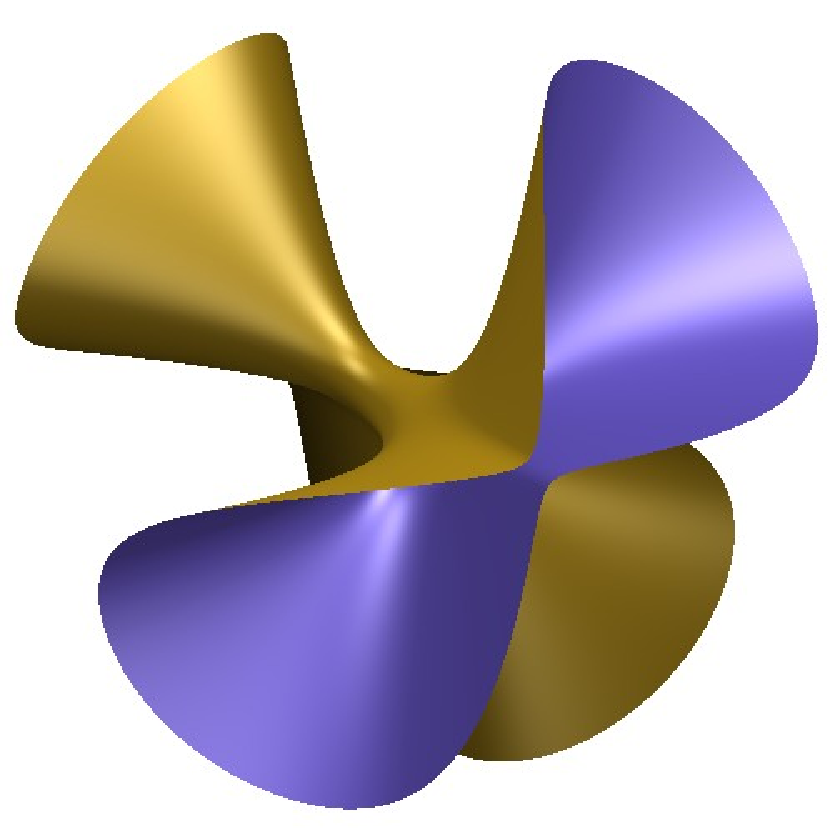
As in Example 4.1, only two components, namely, $V_{\mathit{cor}}(Q_{2})$ and $V_{\mathit{cor}}(Q_{4})$ , contain matrices that represent $\mathcal{L}_{37}$ . The points of $V_{\mathit{cor}}(Q_{2})$ and $V_{\mathit{cor}}(Q_{4})$ have the form $(x,x)$ and $(x,-x)$ , respectively, where $x$ is on the conditional independence surface depicted in Figure 4.1(a).

Example 4.3.

For $\mathcal{L}_{24}=\{12,23|14,24|3\}$ , the ideal $I_{\mathcal{L}_{24}}$ has two prime components:

\displaystyle Q_{1}

\displaystyle=\langle r_{12},r_{23}r_{34}-r_{24},r_{13}r_{14}r_{34}-r_{14}^{2}-r_{34}^{2}+1\rangle,

\displaystyle Q_{2}

\displaystyle=\langle r_{12},r_{23},r_{24}\rangle.

Both of the 3-dimensional components intersect the set of correlation matrices $\mathit{PD}_{4,1}$ , and they intersect each other. Only $V_{\mathit{cor}}(Q_{1})$ contains representing matrices. Note that $V_{\mathit{cor}}(Q_{1})$ is the image of the surface in $(r_{13},r_{14},r_{34})$ -space given by $r_{13}r_{14}r_{34}-r_{14}^{2}-r_{34}^{2}+1=0$ under the transformation setting $r_{24}=r_{23}r_{34}$ and leaving all other coordinates fixed. Figure 4.1(b) displays this surface.

Example 4.4.

For $\mathcal{L}_{28}=\{13|2,14,23|14,24|3\}$ , the ideal $I_{\mathcal{L}_{28}}$ has two 2-dimensional prime components:

\displaystyle Q_{1}

\displaystyle=\langle r_{14},\,r_{12}r_{23}-r_{13},\,r_{23}r_{34}-r_{24},\,r_{12}^{2}+r_{34}^{2}-1\rangle,

\displaystyle Q_{2}

\displaystyle=\langle r_{13},r_{14},r_{23},r_{24}\rangle.

The components intersect $\mathit{PD}_{4,1}$ and each other. The representing set $V_{\mathit{cor}}(Q_{1})$ is the image of a cylinder in $(r_{12},r_{23},r_{34})$ -space under the transformation setting $r_{13}=r_{12}r_{23}$ and $r_{24}=r_{23}r_{34}$ and leaving the other coordinates fixed.

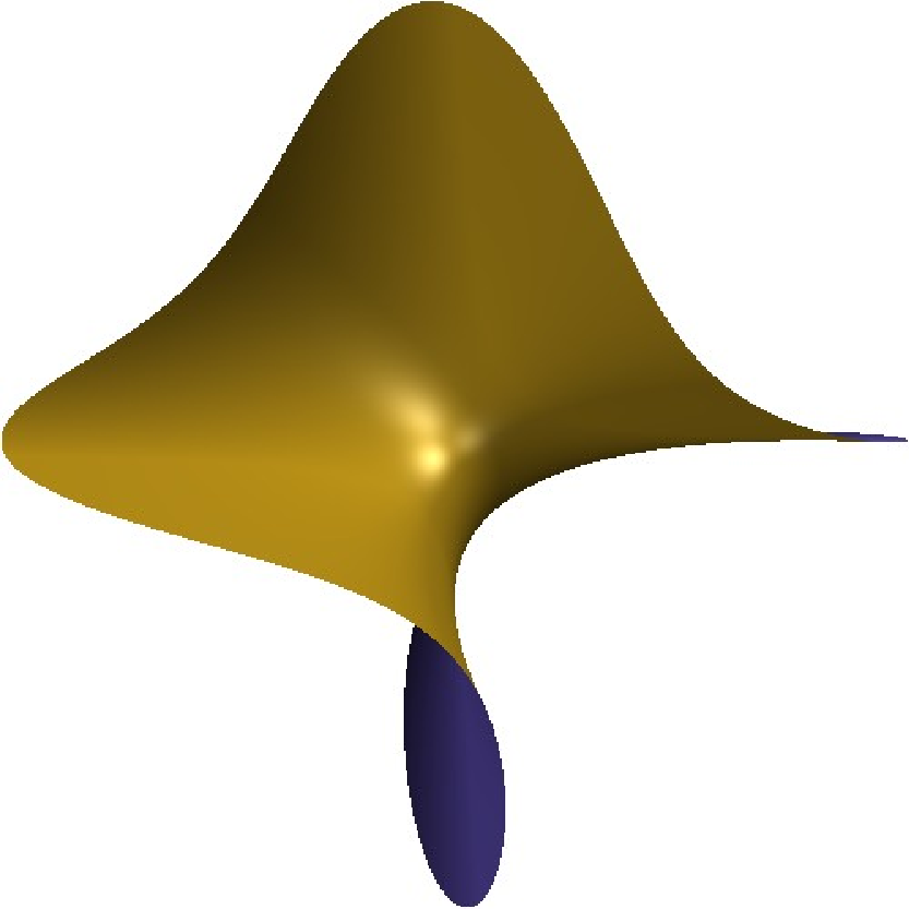
Refer to caption — Figure 4.1. (a) Surface given by $1\mbox{$\perp\kern-5.5pt\perp$}2|3$ , that is, $r_{12}r_{13}-r_{23}=0$ . (b) Surface defined by $r_{13}r_{14}r_{34}-r_{14}^{2}-r_{34}^{2}+1=0$ . It arises for a component of $V_{\mathit{cor}}(\mathcal{L}_{24})=V_{\mathit{cor}}(\{12,23|14,24|3\})$ .

4.2. Singular points

Suppose $V$ is an algebraic variety in the space $\mathbb{S}_{m,1}(\mathbb{C})$ of complex symmetric $m\times m$ matrices with ones on the diagonal. Let $\mathcal{I}(V)$ be the ideal of polynomials vanishing on $V$ . Choose $\{f_{1},f_{2},\ldots,f_{\ell}\}\subset\mathbb{R}[\mathbf{r}]$ to be a finite generating set of $\mathcal{I}(V)$ , and define $J(\mathbf{r})$ to be the $\ell\times\binom{m}{2}$ Jacobian matrix with $(k,ij)$ entry equal to $\partial f_{k}(\mathbf{r})/\partial r_{ij}$ . It can be shown that the maximum rank the Jacobian matrix achieves over $V$ is equal to $\codim(V)=\binom{m}{2}-\dim(V)$ and, in particular, independent of the choice of the generating set $\{f_{1},f_{2},\ldots,f_{\ell}\}$ . See for instance [BR90, §3] for a proof of this fact as we as Lemma 4.1, below.

Definition 4.1.

If the variety $V\subseteq\mathbb{S}_{m,1}(\mathbb{C})$ is irreducible then a matrix $R=(r_{ij})\in V$ is a singular point if the rank of $J(R)$ is smaller than $\codim(V)$ . If $V$ is not irreducible, then the singular points are the singular points of the irreducible components of $V$ together with the points in the intersection of any two irreducible components.

When presented with a set of correlation matrices $V_{\mathit{cor}}(\mathcal{L})$ arising from a CI relation $\mathcal{L}$ , it is useful to study the singularities of the variety $V_{\mathbb{C}}(I_{\mathcal{L}})$ .

Lemma 4.1.

The set of all points in $V_{\mathit{cor}}(\mathcal{L})$ that are non-singular points of $V_{\mathbb{C}}(I_{\mathcal{L}})$ is a smooth manifold.

A computational approach to the smoothness problem is thus to calculate the locus of singular points of $V_{\mathbb{C}}(I_{\mathcal{L}})$ , using for instance the available routines in Singular. To determine irrelevant components that do not intersect the set of correlation matrices $\mathit{PD}_{m,1}$ , we saturate the ideal $S_{\mathcal{L}}$ describing this singular locus on the product of principal minors $D$ and then compute a primary decomposition of $(S_{\mathcal{L}}:D^{\infty})$ . If the singular locus is seen not to intersect $\mathit{PD}_{m,1}$ then the computation proves that $V_{\mathit{cor}}(\mathcal{L})$ is a smooth manifold. If, however, there are correlation matrices that are singular points of $V_{\mathbb{C}}(I_{\mathcal{L}})$ , then we may not yet conclude that $V_{\mathit{cor}}(\mathcal{L})$ is non-smooth around these points. An algebraic obstacle is the fact that $I_{\mathcal{L}}$ might differ from the vanishing ideal $\mathcal{I}(V_{\mathit{cor}}(\mathcal{L}))$ . However, even if $I_{\mathcal{L}}=\mathcal{I}(V_{\mathit{cor}}(\mathcal{L})$ , then algebraic singularity of a point as specified in Definition 4.1 need not imply that the positive definite set $V_{\mathit{cor}}(\mathcal{L})$ fails to be a smooth manifold in a neighborhood of this point. For a classical example of a real algebraic curve with this feature; see [BCR98, Example 3.3.12(b)].

On the three-element set $[m]=[3]$ , and up to equivalence, $\mathcal{L}=\{12,12|3\}$ is the only relation for which $V_{\mathit{cor}}(\mathcal{L})$ is not a smooth manifold. The following proposition explains the drop in rank of the Jacobian in a generalized scenario.

Proposition 4.2.

Let $f_{1}=\det(R_{iC_{1},jC_{1}}),f_{2}=\det(R_{iC_{2},jC_{2}})\in\mathbb{R}[\mathbf{r}]$ be the two determinants encoding the relation $\mathcal{L}=\{ij|C_{1},ij|C_{2}\}$ on $[m]$ . Let $J(R)$ be the $2\times\binom{m}{2}$ Jacobian matrix for $f_{1},f_{2}$ evaluated at a correlation matrix $R$ . Then the maximal rank of $J(R)$ over $V_{\mathit{cor}}(\mathcal{L})$ is two but this rank drops to one exactly when $R$ satisfies the two conditional independence constraints

(4.1)

i\mbox{$\perp\kern-5.5pt\perp$}j(C_{1}\bigtriangleup C_{2})|(C_{1}\cap C_{2})\quad\text{and}\quad j\mbox{$\perp\kern-5.5pt\perp$}i(C_{1}\bigtriangleup C_{2})|(C_{1}\cap C_{2}).

Here, $C_{1}\bigtriangleup C_{2}=(C_{1}\setminus C_{2})\cup(C_{2}\setminus C_{1})$ is the symmetric difference.

Proof.

Let $F=C_{1}\cap C_{2}$ , $C=C_{1}\setminus C_{2}$ and $D=C_{2}\setminus C_{1}$ . Then $C$ , $D$ and $F$ are pairwise disjoint, and $f_{1}=\det(R_{iCF,jCF})$ and $f_{2}=\det(R_{iDF,jDF})$ .

Before turning to the study of the Jacobian $J(R)$ , we note that, by Proposition 1.1, the condition (4.1) is equivalent to the vanishing of five Schur complements:

(4.2)	$\displaystyle r_{ij}-R_{i,F}R_{F,F}^{-1}R_{F,j}$	$\displaystyle=0,$
(4.3)	$\displaystyle R_{C,i}-R_{C,F}R_{F,F}^{-1}R_{F,i}$	$\displaystyle=0,$	$\displaystyle R_{C,j}-R_{C,F}R_{F,F}^{-1}R_{F,j}$	$\displaystyle=0,$
(4.4)	$\displaystyle R_{D,i}-R_{D,F}R_{F,F}^{-1}R_{F,i}$	$\displaystyle=0,$	$\displaystyle R_{D,j}-R_{D,F}R_{F,F}^{-1}R_{F,j}$	$\displaystyle=0.$

Below we sometimes use the following shorthand for such Schur complements:

R_{A,B|F}:=R_{A,B}-R_{A,F}R_{F,F}^{-1}R_{F,B}.

Depending on whether or not $r_{kl}$ is a ‘symmetric’ entry of the matrix defining $f_{h}$ , the partial derivative $\partial f_{h}/\partial r_{kl}$ is equal to the $(k,l)$ cofactor or the sum of the $(k,l)$ and $(l,k)$ cofactors. When discussing these derivatives we always suppress the signs that appear when calculating a cofactor or switching two columns in a determinant. It is easy to check that these signs do not affect the proof. When writing out cofactors we use the notation $|\cdot|=\det(\cdot)$ .

The column of $J(R)$ associated with $r_{ij}$ contains two non-zero entries because

(4.5)

\displaystyle\frac{\partial f_{1}}{\partial r_{ij}}

\displaystyle=|R_{CF,CF}|,

\displaystyle\frac{\partial f_{2}}{\partial r_{ij}}

\displaystyle=|R_{DF,DF}|,

are two principal minors of $R$ . Hence, $J(R)$ has rank either one or two.

Necessity of (4.1): The correlations $r_{ic}$ with $c\in C$ do not appear in $f_{2}$ . Therefore, for the rank of $J(R)$ to drop to one, it is necessary that $\partial f_{1}/\partial r_{ic}=0$ for all $c\in C$ . This derivative is equal to

(4.6)

\frac{\partial f_{1}}{\partial r_{ic}}=\begin{vmatrix}R_{C,j}&R_{C,C\setminus c}&R_{C,F}\\ R_{F,j}&R_{F,C\setminus c}&R_{FF}\end{vmatrix}=\left|R_{FF}\right|\left|R_{C,jC\setminus c}-R_{C,F}R_{F,F}^{-1}R_{F,jC\setminus c}\right|.

(Note that, due to our convention of not distinguishing indices and singleton index set, $jC\setminus c=(C\cup\{j\})\setminus\{c\}$ .) The matrix $R_{C,jC\setminus c}-R_{C,F}R_{F,F}^{-1}R_{F,jC\setminus c}$ is obtained by replacing the $c$ -th column of $R_{C,C|F}$ by $R_{C,j}-R_{C,F}R_{F,F}^{-1}R_{F,j}$ . Since $R_{C,C|F}$ is positive definite, and the last determinant in (4.6) is zero for all $c\in C$ , it follows that $R_{C,j}-R_{C,F}R_{F,F}^{-1}R_{F,j}=0$ . In other words, the second equation in (4.3) holds.

Similarly, the rank of $J(R)$ can only be one if $\partial f_{1}/\partial r_{jc}=0$ for all $c\in C$ . This implies the first equation in (4.3). Treating $f_{2}$ analogously, (4.4) also needs to hold.

The remaining condition, (4.2), is a consequence of the matrix $R$ being in $V_{\mathit{cor}}(\mathcal{L})$ . In the current amended notation, the first defining CI couple is $ij|CF$ . By iterated conditioning (iterated Schur complements), this conditional independence holds if and only if the determinant of the conditional covariance matrix

(4.7)

R_{iC,jC|F}=\begin{bmatrix}R_{i,j|F}&R_{i,C|F}\\ R_{C,j|F}&R_{C,C|F}\end{bmatrix}=\begin{bmatrix}R_{i,j|F}&0\\ 0&R_{C,C|F}\end{bmatrix}

is zero. It follows that $R_{i,j|F}=r_{ij}-R_{i,F}R_{F,F}^{-1}R_{F,j}=0$ , which is (4.2).

Sufficiency of (4.1): If (4.2)-(4.4) hold, many partial derivatives are zero. First, (4.6) implies $\partial f_{1}/\partial r_{ic}=\partial f_{1}/\partial r_{jc}=\partial f_{2}/\partial r_{id}=\partial f_{2}/\partial r_{jd}=0$ for $c\in C$ and $d\in D$ .

Second, consider two distinct indices $c,c^{\prime}\in C$ . The derivative $\partial f_{1}/\partial r_{cc^{\prime}}$ is the sum of two cofactors. The first cofactor is

\displaystyle\begin{vmatrix}R_{iC\setminus c,jC\setminus c^{\prime}}&R_{iC\setminus c,F}\\ R_{F,jC\setminus c^{\prime}}&R_{F,F}\end{vmatrix}=\left|R_{F,F}\right|\begin{vmatrix}R_{i,j|F}&R_{i,C\setminus c^{\prime}|F}\\ R_{C\setminus c,j|F}&R_{C\setminus c,C\setminus c^{\prime}|F}\end{vmatrix}=0,

because, by (4.2) and (4.3), the last determinant is that of a matrix with first row and column zero. The other cofactor is obtained by switching $c$ and $c^{\prime}$ and also zero. Hence, $\partial f_{1}/\partial r_{cc^{\prime}}=0$ . Similarly, $\partial f_{2}/\partial r_{dd^{\prime}}=0$ for two distinct indices $d,d^{\prime}\in D$ .

Third, if $c\in C$ and $f\in F$ , then $\partial f_{1}/\partial r_{cf}$ is the sum of two cofactors. Using (4.2) and (4.3), one cofactor is seen to be

\displaystyle\begin{vmatrix}R_{i,C}&R_{i,F\setminus f}&r_{ij}\\ R_{C\setminus c,C}&R_{C\setminus c,F\setminus f}&R_{C\setminus c,j}\\ R_{F,C}&R_{F,F\setminus f}&R_{F,j}\end{vmatrix}=\begin{vmatrix}R_{i,F}R_{F,F}^{-1}R_{F,C}&R_{i,F\setminus f}&R_{i,F}R_{F,F}^{-1}R_{F,j}\\ R_{C\setminus c,C}&R_{C\setminus c,F\setminus f}&R_{C\setminus c,F}R_{F,F}^{-1}R_{F,j}\\ R_{F,C}&R_{F,F\setminus f}&R_{F,F}R_{F,F}^{-1}R_{F,j}\end{vmatrix}.

Let $R_{F,F}^{-1}R_{F,j}(f)$ be the $f$ -th entry of the vector $R_{F,F}^{-1}R_{F,j}$ . The above cofactor is

\displaystyle R_{F,F}^{-1}R_{F,j}(f)\,\cdot\,\begin{vmatrix}R_{i,F}R_{F,F}^{-1}R_{F,C}&R_{i,F}R_{F,F}^{-1}R_{F,F}\\ R_{C\setminus c,C}&R_{C\setminus c,F}\\ R_{F,C}&R_{F,F}\end{vmatrix}=0

because $(R_{i,F}R_{F,F}^{-1}R_{F,C},\,R_{i,F}R_{F,F}^{-1}R_{F,F})$ is a linear combination of rows of the matrix $(R_{F,C},\,R_{F,F})$ . Similarly, the other cofactor is zero and, thus, $\partial f_{1}/\partial r_{cf}=0$ . The vanishing of $\partial f_{2}/\partial r_{df}$ for $d\in D$ is analogous.

Our calculations show that only the columns of $J(R)$ associated with $r_{ij}$ , $r_{if}$ , $r_{jf}$ and $r_{ff^{\prime}}$ for $f\neq f^{\prime}\in F$ may be non-zero. To establish that $J(R)$ has rank one we show that these columns are all multiples of the one for $r_{ij}$ given in (4.5).

Using the second equation in (4.3), we have that

\displaystyle\frac{\partial f_{1}}{\partial r_{if}}

\displaystyle=\begin{vmatrix}R_{C,C}&R_{C,F\setminus f}&R_{C,j}\\ R_{F,C}&R_{F,F\setminus f}&R_{Fj}\end{vmatrix}=\begin{vmatrix}R_{C,C}&R_{C,F\setminus f}&R_{C,F}R_{F,F}^{-1}R_{F,j}\\ R_{F,C}&R_{F,F\setminus f}&R_{F,F}R_{F,F}^{-1}R_{Fj}\end{vmatrix}.

Therefore, we obtain that

\displaystyle\frac{\partial f_{1}}{\partial r_{if}}

\displaystyle=R_{F,F}^{-1}R_{F,j}(f)\,\cdot\,\begin{vmatrix}R_{C,C}&R_{C,F}\\ R_{F,C}&R_{F,F}\end{vmatrix}=R_{F,F}^{-1}R_{F,j}(f)\,\frac{\partial f_{1}}{\partial r_{ij}}.

The derivatives $\partial f_{1}/\partial r_{jf}$ , $\partial f_{2}/\partial r_{if}$ and $\partial f_{2}/\partial r_{jf}$ are similar multiples of the corresponding derivatives with respect to $r_{ij}$ .

The two remaining cases $\partial f_{1}/\partial r_{ff^{\prime}}$ and $\partial f_{2}/\partial r_{ff^{\prime}}$ are again analogous, and we only consider the former. This derivative is the sum of two cofactors, one being

\displaystyle\begin{vmatrix}R_{i,C}&R_{i,F\setminus f^{\prime}}&r_{ij}\\ R_{C,C}&R_{C,F\setminus f^{\prime}}&R_{C,j}\\ R_{F\setminus f,C}&R_{F\setminus f,F\setminus f^{\prime}}&R_{F\setminus f,j}\end{vmatrix}=\begin{vmatrix}R_{i,C}&R_{i,F\setminus f^{\prime}}&R_{i,F}R_{F,F}^{-1}R_{F,j}\\ R_{C,C}&R_{C,F\setminus f^{\prime}}&R_{C,F}R_{F,F}^{-1}R_{F,j}\\ R_{F\setminus f,C}&R_{F\setminus f,F\setminus f^{\prime}}&R_{F\setminus f,F}R_{F,F}^{-1}R_{F,j}\end{vmatrix}

where (4.2) and the second equation in (4.3) were applied. Using the first equation in (4.3), the cofactor is seen to be equal to

	$\displaystyle R_{F,F}^{-1}R_{F,j}(f^{\prime})$	$\displaystyle\,\cdot\,\begin{vmatrix}R_{i,F}R_{F,F}^{-1}R_{F,C}&R_{F,F}R_{F,F}^{-1}R_{i,F}\\ R_{C,C}&R_{C,F}\\ R_{F\setminus f,C}&R_{F\setminus f,F}\end{vmatrix}$
		$\displaystyle=R_{F,F}^{-1}R_{F,j}(f^{\prime})\,\cdot\,R_{F,F}^{-1}R_{F,i}(f)\,\cdot\,\begin{vmatrix}R_{C,C}&R_{C,F}\\ R_{F,C}&R_{F,F}\end{vmatrix}$

The other cofactor is obtained by switching $f$ and $f^{\prime}$ and, thus,

\displaystyle\frac{\partial f_{1}}{\partial r_{ff^{\prime}}}

\displaystyle=\left[R_{F,F}^{-1}R_{F,j}(f^{\prime})\,\cdot\,R_{F,F}^{-1}R_{F,i}(f)+R_{F,F}^{-1}R_{F,j}(f)\,\cdot\,R_{F,F}^{-1}R_{F,i}(f^{\prime})\right]\,\frac{\partial f_{1}}{\partial r_{ij}}.

We have thus proven that the rank of $J(R)$ is one when (4.1) holds. ∎

4.3. Singular loci of representable models on four variables

Implementing the computational approach described in Section 4.2, we find the following result for $m=4$ random variables. Note that Proposition 4.2 applies to the representable relations with index 29 and 32.

Theorem 4.1.

If $\mathcal{L}$ is a representable relation on $[m]=[4]$ , then $V_{\mathit{cor}}(\mathcal{L})$ is a smooth manifold unless $\mathcal{L}$ is equivalent to one of 12 relations $\mathcal{L}_{i}$ with index $i\in\{14,15,20,24,28,29,30,32,36,37,46,51\}$ listed in Table A.1.

Proof.

Going through 53 possible cases, the computation identifies 41 models as smooth according to Lemma 4.1. The remaining 12 models are algebraically singular. Our analysis of tangent cones below shows that these 12 models are indeed not smooth manifolds (compare Theorem 4.2). ∎

We now give some more details on the singularities of the 12 relations listed in Theorem 4.1. They can be grouped into 3 categories:

(a) Union of smooth components: If $i\in\{24,28\}$ then $V_{\mathit{cor}}(\mathcal{L}_{i})$ is the union of two components that are both smooth manifolds; compare Examples 4.3 and 4.4. In each case the singular locus is simply the intersection of the two components, which gives the surface defined by $\langle r_{12},r_{23},r_{24},r_{13}r_{14}r_{34}-r_{14}^{2}-r_{34}^{2}+1\rangle$ and the circle defined by $\langle r_{13},r_{14},r_{23},r_{24},r_{12}^{2}+r_{34}^{2}-1\rangle.$

If $i\in\{15,37\}$ then $V_{\mathit{cor}}(\mathcal{L}_{i})$ is the union of four smooth components; compare Examples 4.1 and 4.2. The singular locus is again obtained by forming intersections of components. In each case the singular locus has 4 components that for $i=15$ are given by

		$\displaystyle\langle r_{12},r_{14},r_{23},r_{34},r_{13}-r_{24}\rangle,$	$\displaystyle\langle r_{12},r_{14},r_{23},r_{34},r_{13}+r_{24}\rangle,$
		$\displaystyle\langle r_{13},r_{14},r_{23},r_{24},r_{12}-r_{34}\rangle,$	$\displaystyle\langle r_{13},r_{14},r_{23},r_{24},r_{12}+r_{34}\rangle,$

and for $i=37$ by

		$\displaystyle\langle r_{12},r_{13},r_{24},r_{34},r_{14}-r_{23}\rangle,$	$\displaystyle\langle r_{12},r_{13},r_{24},r_{34},r_{14}+r_{23}\rangle,$
		$\displaystyle\langle r_{12},r_{14},r_{23},r_{34},r_{13}-r_{24}\rangle,$	$\displaystyle\langle r_{12},r_{14},r_{23},r_{34},r_{13}+r_{24}\rangle.$

(b) Singular at identity matrix: The six models with $i\in\{14,20,30,36,46,51\}$ , have the identity matrix as their only singular point.

(c) Singular at almost diagonal matrices: Two cases remain. If $i=29$ , the correlation matrices that are singularities have the entries other than $r_{14}$ equal to zero. For $i=32$ , the singularities have the entries other than $r_{34}$ equal to zero.

Since algebraic singularity need not imply failure of smoothness, we now study the local geometry of the sets $V_{\mathit{cor}}(\mathcal{L})$ at their algebraic singularities. This local geometry is represented by the tangent cone, which is also related to asymptotic distribution theory for statistical tests [Drt09].

Definition 4.2.

A tangent direction of $V_{\mathit{cor}}(\mathcal{L})$ at the correlation matrix $R_{0}\in\mathit{PD}_{m,1}$ is a matrix in $\mathbb{R}^{m\times m}$ that is the limit of a sequence $\alpha_{n}(R_{n}-R_{0})$ , where the $\alpha_{n}$ are positive reals and the $R_{n}\in V_{\mathit{cor}}(\mathcal{L})$ converge to $R_{0}$ . The tangent cone $\mathit{TC}_{\mathcal{L}}(R_{0})$ is the closed cone made up of all these tangent directions.

The representable relations $\mathcal{L}_{i}$ with $i\in\{15,24,28,37\}$ define unions of smooth manifolds. Their singularities lie in the intersection of two or more of the smooth components, and the tangent cone is then simply the union of the tangent spaces of the smooth components containing a considered singularity.

Our strategy to determine the tangent cones of the remaining 8 singular representable models is again algebraic. Let the correlation matrix $R_{0}\in\mathit{PD}_{m,1}$ correspond to a root of the polynomial $f\in\mathbb{R}[\mathbf{r}]$ . Write

f(R)\,=\,\sum_{h=l}^{L}f_{h}(R-R_{0})

as a sum of homogeneous polynomials $f_{h}$ in $R-R_{0}$ , where $f_{h}(t)$ has degree $h$ and $f_{l}\not=0$ . Since $f(R_{0})=0$ , the minimal degree $l$ is at least one, and we define $f_{R_{0},\min}=f_{l}$ . The algebraic tangent cone of $V_{\mathit{cor}}(\mathcal{L})$ at $R_{0}$ is the real algebraic variety defined by the tangent cone ideal

(4.8)

\left\{f_{R_{0},\min}\;:\;f\in\mathcal{I}(V_{\mathit{cor}}(\mathcal{L}))\right\}\subset\mathbb{R}[\mathbf{r}].

The algebraic tangent cone contains the tangent cone $\mathit{TC}_{\mathcal{L}}(R_{0})$ ; see e.g. [DSS09, §2.3]. In our setup we work with the ideal $I_{\mathcal{L}}\subseteq\mathcal{I}(V_{\mathit{cor}}(\mathcal{L}))$ and, thus, consider the cone $\mathit{AC}_{\mathcal{L}}(R_{0})$ given by the real algebraic variety of the ideal

(4.9)

C_{\mathcal{L}}(R_{0})=\left\{f_{R_{0},\min}\;:\;f\in I_{\mathcal{L}}\right\}\subset\mathbb{R}[\mathbf{r}].

The cone $\mathit{AC}_{\mathcal{L}}(R_{0})$ always contains the algebraic tangent cone. Therefore, we still have the inclusion $\mathit{TC}_{\mathcal{L}}(R_{0})\subseteq\mathit{AC}_{\mathcal{L}}(R_{0})$ . The ideal $C_{\mathcal{L}}(R_{0})$ in (4.9) can be computed using Gröbner basis methods that are implemented, for instance, in the tangentcone command in Singular.

Theorem 4.2.

If $\mathcal{L}_{i}$ is one of the 8 representable relations on $[m]=[4]$ with index $i\in\{14,20,29,30,32,36,46,51\}$ , then at all singularities $R_{0}$ of $V_{\mathit{cor}}(\mathcal{L}_{i})$ the tangent cone $\mathit{TC}_{\mathcal{L}}(R_{0})$ is equal to the algebraically defined cone $\mathit{AC}_{\mathcal{L}}(R_{0})$ . In particular, the models $V_{\mathit{cor}}(\mathcal{L}_{i})$ are indeed non-smooth.

Proof.

The six models with $i\in\{14,20,30,36,46,51\}$ , have the identity matrix $\mathit{Id}$ as their only singular correlation matrix. The cone ideals are

(4.10)	$\displaystyle C_{\mathcal{L}_{14}}(\mathit{Id})=C_{\mathcal{L}_{46}}(\mathit{Id})$	$\displaystyle=\langle r_{14},r_{23},r_{12}r_{24}+r_{13}r_{34}\rangle,$
(4.11)	$\displaystyle C_{\mathcal{L}_{20}}(\mathit{Id})=C_{\mathcal{L}_{51}}(\mathit{Id})$	$\displaystyle=\langle r_{14},r_{23},r_{12}r_{24}-r_{13}r_{34}\rangle,$
(4.12)	$\displaystyle C_{\mathcal{L}_{30}}(\mathit{Id})$	$\displaystyle=\langle r_{14},r_{23},r_{12}r_{13}-r_{24}r_{34}\rangle,$
(4.13)	$\displaystyle C_{\mathcal{L}_{36}}(\mathit{Id})$	$\displaystyle=\langle r_{12},r_{34},r_{13}r_{23}-r_{14}r_{24}\rangle.$

The latter three ideals are equivalent under permutation of the indices in $[m]=[4]$ .

For $\mathcal{L}_{29}$ , the singular points $R_{0}=(\rho_{ij}^{0})$ have all off-diagonal entries zero except for possibly $\rho_{14}^{0}$ which can be any number in $(-1,1)$ . The cone ideal varies continuously with $\rho_{14}^{0}$ :

(4.14)

\displaystyle C_{\mathcal{L}_{29}}(R_{0})

\displaystyle=\langle\;r_{23},\,r_{13}(r_{12}-\rho_{14}^{0}r_{24})+r_{34}(r_{24}-\rho_{14}^{0}r_{12})\;\rangle.

The algebraic cones in this family can be transformed into each other by an invertible linear transformation.

For $\mathcal{L}_{32}$ , the singular points $R_{0}=(\rho_{ij}^{0})$ have all off-diagonal entries zero except for possibly $\rho_{34}^{0}$ which can be any number in $(-1,1)$ . The cone ideal, however, does not depend on the value of $\rho_{34}^{0}$ :

(4.15)

C_{\mathcal{L}_{32}}(R_{0})=\langle r_{12},r_{13}r_{23}-r_{14}r_{24}\rangle.

In each case, it can be shown that all vectors in $\mathit{AC}_{\mathcal{L}_{i}}(R_{0})$ are indeed tangent directions for $V_{\mathit{cor}}(\mathcal{L}_{i})$ . We prove the result for $i=29$ ; the other 7 cases are similar.

Tangent cone of $V_{\mathit{cor}}(\mathcal{L}_{29})$ : The ideal

I_{\mathcal{L}_{29}}=\langle r_{23},-r_{14}^{2}r_{23}+r_{13}r_{14}r_{24}+r_{12}r_{14}r_{34}-r_{12}r_{13}-r_{24}r_{34}+r_{23}\rangle.

Let $\boldsymbol{r}_{0}=(0,0,\rho,0,0,0)$ with $|\rho|<1$ be a singular point and $R_{0}$ the corresponding correlation matrix. Both $TC_{\mathcal{L}_{29}}(R_{0})$ and $AC_{\mathcal{L}_{29}}(R_{0})$ are closed sets, and we may thus consider a generic direction $\boldsymbol{t}=(t_{12},t_{13},t_{14},t_{23},t_{24},t_{34})$ in the cone $AC_{\mathcal{L}_{29}}(R_{0})$ given by the ideal $C_{\mathcal{L}_{29}}(R_{0})$ in (4.14). We may assume $\rho t_{12}-t_{24}\neq 0$ , and obtain

(4.16)

\boldsymbol{t}=\left(t_{12},t_{13},t_{14},0,t_{24},\frac{t_{13}(t_{12}-\rho t_{24})}{\rho t_{12}-t_{24}}\right).

Let

\boldsymbol{r}_{n}=\left(\frac{t_{12}}{n},\frac{t_{13}}{n},\rho+\frac{t_{14}}{n},0,\frac{t_{24}}{n},\frac{nt_{13}(t_{12}-\rho t_{24})-t_{13}t_{14}t_{24}}{n^{2}(\rho t_{12}-t_{24})+nt_{12}t_{14}}\right).

It is easy to show that $\boldsymbol{r}_{n}\in V_{\mathit{cor}}(\mathcal{L}_{29})$ for large $n$ ; and $\boldsymbol{r}_{n}\rightarrow\boldsymbol{r}_{0}$ and $n(\boldsymbol{r}_{n}-\boldsymbol{r}_{0})\rightarrow\boldsymbol{t}$ as $n\rightarrow\infty$ . Thus, $\boldsymbol{t}\in TC_{\mathcal{L}_{29}}(R_{0})$ , and it follows that $TC_{\mathcal{L}_{29}}(R_{0})=AC_{\mathcal{L}_{29}}(R_{0})$ . ∎

5. Conclusion

We conclude by pointing out some interesting features of our computational results for $m=4$ . First, the model associated with a representable relation need not correspond to an irreducible variety. It can be a union of several distinct irreducible components that all intersect the cone of positive definite matrices; see Examples 4.3 and 4.4 in which the components all have the same dimension.

Second, Examples 4.3 and 4.4 also provide a negative answer to Question 7.11 in [DSS09]. This question asked whether Gaussian conditional independence models that are smooth locally at the identity matrix are smooth manifolds. The singular loci of these examples, however, do not contain the identity matrix. All other singular models are singular at the identity matrix, and in fact, the identity matrix is often the only singularity (recall Section 4.3).

Our final comment is based on the observation that Gaussian conditional independence models for $m=3$ variables are smooth except for the model given by $ij$ and $ij|k$ , and that singular models can arise more generally when combining two CI couples $ij|C$ and $ij|D$ (recall Proposition 4.2). This observation may lead one to guess that if a complete relation $\mathcal{L}$ does not contain two CI couples $ij|C$ and $ij|D$ that repeat the pair $ij$ , then the model $V_{\mathit{pd}}(\mathcal{L})$ is smooth. Unfortunately, this is false, again because of Examples 4.3 and 4.4.

Appendix A Lists of relations and CI implications

In this appendix we provide encyclopedic information about conditional independence of four Gaussian random variables. This comprehends the listing of all representable and complete relations, as well as all Gaussian CI implications.

A.1. Representable and complete relations

Counting up to equivalence, there are 53 representable relations on four variables. They are listed in Table A.1 below, where the symbol $\ast$ is used to denote all possible conditioning sets. With this convention, the symbol $12|\ast$ , for instance, expands to $\{12,12|3,12|4,12|34\}$ . In the table we indicate whether the model is singular and give the equivalent dual of each representable relation. We include a permutation of the indices that provides the equivalence. Using cycle notation, an empty entry stands for the identity.

The remaining $101-53=48$ equivalence classes of complete but not representable relations are listed in Table A.2. Each cell in the second column provides, row-by-row, the representable relations in the minimal representable decomposition from Theorem 2.1. Their intersection gives the considered complete relation. For each representable relation in the table cell, we also provide, in the third column, the label of its equivalent representable relation in Table A.1 and the permutation that transforms the equivalent relation to the current one.

In the introduction we mentioned that graphical models are smooth CI models. Over 4 nodes, there are 11 unlabelled undirected graphs. Figure 2.1 from Section 2.2 shows for each of the 10 non-empty graphs the corresponding representable relation from Table A.1. Up to equivalence, there are 10 additional graphical models associated with acyclic digraphs on 4 nodes. The 10 digraphs are shown in Figure A.1 together with the corresponding representable relations. We remark that the representable relations $\mathcal{L}_{35}$ , $\mathcal{L}_{40}$ , $\mathcal{L}_{44}$ , $\mathcal{L}_{48}$ and $\mathcal{L}_{49}$ determine graphical models based on mixed graphs with directed and bi-directed edges. The corresponding 5 graphs are shown in [RS03, Fig. 10]. Two further representable relations correspond to chain graphs: $\mathcal{L}_{13}$ is given by the so-called LWF interpretation of the graph in [AMP01, Fig. 1] and $\mathcal{L}_{43}$ by the AMP interpretation of the graph in [AMP01, Fig. 8(a)].

A.2. All CI implications for four variables

Although not pointed out explicitly, [LM07] have proved the following result via Theorem 2.4.

Theorem A.1.

For $m=4$ variables, all the Gaussian CI implications follow from the implications (2.3)-(2.10) and the weak transitivity property in (2.11).

Due to its disjunctive conclusion, the weak transitivity property is not a CI implication in the sense of our strict Definition 2.2. A natural problem is thus to find a set of CI implications in the sense of this definition, from which all other such CI implications can be deduced.

Recall the last step of the search of complete relations in Section 2, which treats 94 semigaussoids that satisfy (2.6)-(2.10) but are not representable. Of these, 46 are not complete and each yield new CI implications. Namely, if $\mathcal{L}$ is such a semi-gaussoid and $\bar{\mathcal{L}}$ the smallest complete relation containing $\mathcal{L}$ , then $\mathcal{L}\Rightarrow(\bar{\mathcal{L}}\setminus\mathcal{L})$ . After a careful check, we find that the following 13 CI implications together with their duals generate all of the 46 CI implications given by the non-complete semigaussoids:

(A.1)	$\displaystyle\{23\|4,23\|14,24\|1,34\|1\}$	$\displaystyle\quad\Longrightarrow\quad\{23,23\|1,24\|13,34\|12\},$
(A.2)	$\displaystyle\{23,23\|1,24\|1,34\|1\}$	$\displaystyle\quad\Longrightarrow\quad\{23\|4,23\|14,24\|13,34\|12\},$
(A.3)	$\displaystyle\{14\|2,14\|3,14\|23,23\|14\}$	$\displaystyle\quad\Longrightarrow\quad\{14\},$
(A.4)	$\displaystyle\{14,14\|2,14\|23,23\|14\}$	$\displaystyle\quad\Longrightarrow\quad\{14\|3\},$
(A.5)	$\displaystyle\{14,14\|2,14\|3,23\|14\}$	$\displaystyle\quad\Longrightarrow\quad\{14\|23\},$
(A.6)	$\displaystyle\{14,14\|23,23\|1,23\|14\}$	$\displaystyle\quad\Longrightarrow\quad\{14\|2,14\|3\},$
(A.7)	$\displaystyle\{14\|2,14\|3,23\|1,23\|14\}$	$\displaystyle\quad\Longrightarrow\quad\{14,14\|23\},$
(A.8)	$\displaystyle\{12,14\|3,14\|23,23\|14\}$	$\displaystyle\quad\Longrightarrow\quad\{12\|3,12\|4,12\|34,23\|4\},$
(A.9)	$\displaystyle\{12,14\|3,23\|4,23\|14\}$	$\displaystyle\quad\Longrightarrow\quad\{12\|3,12\|4,12\|34,14\|23\},$
(A.10)	$\displaystyle\{12\|3,14\|2,23\|4,23\|14\}$	$\displaystyle\quad\Longrightarrow\quad\{12,12\|4,12\|34,14\},$
(A.11)	$\displaystyle\{12\|3,14,14\|2,23\|14\}$	$\displaystyle\quad\Longrightarrow\quad\{12,12\|4,12\|34,23\|4\},$
(A.12)	$\displaystyle\{14\|2,23\|1,23\|4,23\|14\}$	$\displaystyle\quad\Longrightarrow\quad\{23\},$
(A.13)	$\displaystyle\{14\|2,23,23\|1,23\|14\}$	$\displaystyle\quad\Longrightarrow\quad\{23\|4\}.$

Although the CI implications (A.1)-(A.13) are written with concrete choices of indices, they should be viewed as representing an equivalence class, that is, as the class of implications that can be obtained by a permutation of the indices.

Theorem A.2.

A relation on $[m]=[4]$ is complete if and only if it satisfies the CI implications (2.3)-(2.10), (A.1)-(A.13) and the duals of (A.1)-(A.13).

Corollary A.1.

All Gaussian CI implications for 4 variables can be deduced from (2.3)-(2.10), (A.1)-(A.13) and the duals of (A.1)-(A.13).

We conclude by demonstrating how to prove some of the implications in (A.1)-(A.13) by using the weak transitivity property.

Proof of (A.1).

Suppose the CI statements in the relation on the left hand side are satisfied. By (2.3), $\{24|1,34|1\}\Rightarrow\{24|13,34|12\}$ . By (2.4), $\{24|1,23|41\}\Rightarrow\{23|1,24|13\}$ . Hence, it remains to show that $23$ is implied. By weak transitivity applied to $\{23|4,23|14\}$ , we conclude that $12|4$ or $13|4$ hold. There are two cases:

(i)

Suppose that $12|4$ holds. Then $\{12|4,24|1\}\Rightarrow\{12,24\}$ by the ‘intersection’ implication in (2.5). Applying (2.4) again, $\{12,23|1\}\Rightarrow\{23\}$ .
(ii)

By symmetry, we reach the conclusion that $23$ holds also when starting from $13|4$ instead of $12|4$ . ∎

Proof of (A.6).

In view of (A.4) (interchange 2 and 3 when necessary), we only need to show $14|2$ or $14|3$ must hold when the CI statements on the left hand side hold. From weak transitivity applied to $\{23|1,23|14\}$ , two cases arise:

(i)

If $24|1$ holds then we may apply (2.3) to obtain $\{24|1,23|1\}\Rightarrow\{24|13\}$ . By (2.5), $\{24|13,14|23\}\Rightarrow\{14|3\}$ .
(ii)

If $34|1$ holds then we may conclude, by symmetry, that $14|2$ holds. ∎

Proof of (A.9).

It suffices to show that $12|3$ and $12|4$ are implied. Applying weak transitivity to $\{23|4,23|14\}$ we can consider the two cases $12|4$ or $13|4$ :

(i)

If $13|4$ holds then by (2.5), $\{13|4,14|3\}\Rightarrow\{13,14\}$ . Using (2.3), we can conclude $\{12,13,14\}\Rightarrow\{12|3,12|4\}$ .
(ii)
If $12|4$ holds then we can apply weak transitivity to $\{12,12|4\}$ . The two subcases are:
1. (ii-a)
  
  If $24$ holds then, by (2.4), $\{24,23|4\}\Rightarrow\{23\}$ and, by (2.3), $\{12,24\}\Rightarrow\{12|4\}$ . Another application of (2.3) yields $\{12,23\}\Rightarrow\{12|3\}$ .
2. (ii-b)
  If $14$ holds then we may apply weak transitivity to $\{14,14|3\}$ and split into two further subcases:
  1. (ii-b1)
    
    If $13$ holds, then (2.3) yields $\{12,13\}\Rightarrow\{12|3\}$ .
  2. (ii-b2)
    
    If $34$ holds, then (2.4) yields $\{34,23|4\}\Rightarrow\{23\}$ . Applying (2.3) we conclude $\{12,23\}\Rightarrow\{12|3\}$ . ∎

Proof of (A.10).

Since $\{12,14|2\}\Rightarrow\{14,12|4\}$ by (2.4) and $\{12|4,23|4\}\Rightarrow\{12|34\}$ by (2.3), it suffices to show that $12$ holds under the assumed CI statements on the left hand side. Apply weak transitivity to $\{23|4,23|14\}$ to obtain two cases:

(i)

If $12|4$ holds then (2.5) yields $\{12|4,14|2\}\Rightarrow\{12\}$ .
(ii)

If $13|4$ holds then (2.9) yields $\{13|4,14|2,12|3\}\Rightarrow\{12\}$ . ∎

Table A.1. All representable relations on four variables, up to equivalence.

$i$	Elements of $\mathcal{L}_{i}$	Singular	Dual
1	$12\|\ast$ , $13\|\ast$ , $14\|\ast$ , $23\|\ast$ , $24\|\ast$ , $34\|\ast$		1
2	$13\|\ast$ , $14\|\ast$ , $23\|\ast$ , $24\|\ast$ , $34\|\ast$		2
3	$14\|\ast$ , $23\|1$ , $23\|14$ , $24\|\ast$ , $34\|\ast$		38
4	$13\|\ast$ , $14\|\ast$ , $23\|\ast$ $24\|\ast$		4
5	$14\|\ast$ , $24\|\ast$ , $34\|\ast$		5
6	$23\|1$ , $23\|14$ , $24\|1$ , $24\|13$ , $34\|1$ , $34\|12$		39
7	$14\|2$ , $14\|23$ , $23\|1$ , $23\|14$ , $34\|1$ , $34\|2$ , $34\|12$		40
8	$23\|1$ , $23\|14$ , $34\|1$ , $34\|12$		41
9	$23\|1$ , $23\|14$ , $24\|3$ , $34\|1$ , $34\|12$		42
10	$12$ , $12\|3$ , $23$ , $23\|1$ , $23\|14$ , $34\|1$ , $34\|12$		10	(14)(23)
11	$23\|1$ , $23\|14$ , $24$ , $34\|1$ , $34\|12$		43
12	$14\|23$ , $23\|14$		44
13	$12$ , $14\|23$ , $23\|14$		45
14	$14$ , $14\|23$ , $23\|14$	✓	46
15	$14$ , $14\|23$ , $23$ , $23\|14$	✓	15
16	$23\|14$		47
17	$12\|3$ , $23\|14$		48
18	$14\|2$ , $23\|14$		49
19	$12\|3$ , $14\|2$ , $23\|14$		50
20	$14\|2$ , $14\|3$ , $23\|14$	✓	51
21	$13\|2$ , $23\|14$ , $24\|3$		52
22	$12$ , $23\|14$		22	(13)
23	$12$ , $14\|3$ , $23\|14$		25	(13)
24	$12$ , $23\|14$ , $24\|3$	✓	24	(13)
25	$12$ , $23\|14$ , $34\|2$		23	(13)
26	$14$ , $23\|14$		26	(12)(34)
27	$12\|3$ , $14$ , $23\|14$		27	(12)(34)
28	$13\|2$ , $14$ , $23\|14$ , $24\|3$	✓	28	(13)(24)
29	$23$ , $23\|14$	✓	29
30	$14\|2$ , $23$ , $23\|14$	✓	30	(23)
31	$12\|3$		31	(34)
32	$12\|3$ , $12\|4$	✓	32
33	$12\|3$ , $13\|4$		33	(23)
34	$12\|3$ , $14\|2$ , $23\|4$		34	(12)(34)
35	$12\|3$ , $34\|1$		35	(12)(34)
36	$12\|3$ , $12\|4$ , $34\|1$	✓	36	(12)
37	$12\|3$ , $12\|4$ , $34\|1$ , $34\|2$	✓	37
38	$14\|\ast$ , $23$ , $23\|4$ , $24\|\ast$ , $34\|\ast$		3
39	$23$ , $23\|4$ , $24$ , $24\|3$ , $34$ , $34\|2$		6
40	$14$ , $14\|3$ , $23$ , $23\|4$ , $34$ , $34\|1$ , $34\|2$		7
41	$23$ , $23\|4$ , $34$ , $34\|2$		8
42	$23$ , $23\|4$ , $24\|1$ , $34$ , $34\|2$		9
43	$23$ , $23\|4$ , $24\|13$ , $34$ , $34\|2$		11
44	$14$ , $23$		12
45	$12\|34$ , $14$ , $23$		13
46	$14$ , $14\|23$ , $23$	✓	14
47	$23$		16
48	$12\|4$ , $23$		17
49	$14\|3$ , $23$		18
50	$12\|4$ , $14\|3$ , $23$		19
51	$14\|2$ , $14\|3$ , $23$	✓	20
52	$13\|4$ , $23$ , $24\|1$		21
53	$\emptyset$		53

Table A.2. All complete non-representable relations on four variables, up to equivalence.

$i$	Representable decomposition of $\mathcal{L}_{i}$	Equivalence class
54	$13\|\ast$ , $14\|\ast$ , $23\|\ast$ , $24\|\ast$ , $34\|\ast$	2
	$12\|\ast$ , $14\|\ast$ , $23\|\ast$ , $24\|\ast$ , $34\|\ast$	2	(234)
55	$13\|\ast$ , $23\|\ast$ , $24\|1$ , $24\|13$ , $34\|\ast$	3	(34)
	$12\|\ast$ , $23\|\ast$ , $24\|\ast$ , $34\|1$ , $34\|12$	3	(234)
56	$13\|\ast$ , $14\|\ast$ , $23\|\ast$ , $24\|\ast$ , $34\|\ast$	2
	$12\|\ast$ , $23\|\ast$ , $24\|\ast$ , $34\|1$ , $34\|12$	3	(234)
57	$13\|\ast$ , $14\|\ast$ , $23\|\ast$ , $24\|\ast$ , $34\|\ast$	2
	$12\|\ast$ , $14\|\ast$ , $23\|\ast$ , $24\|\ast$ , $34\|\ast$	2	(234)
	$12\|\ast$ , $13\|\ast$ , $23\|\ast$ , $24\|\ast$ , $34\|\ast$	2	(24)
58	$14\|\ast$ , $23\|1$ , $23\|14$ , $24\|\ast$ , $34\|\ast$	3
	$13\|\ast$ , $14\|2$ , $14\|23$ , $23\|\ast$ , $34\|\ast$	3	(1243)
	$12\|\ast$ , $14\|\ast$ , $23\|\ast$ , $34\|\ast$	4	(234)
59	$14\|\ast$ , $23\|1$ , $23\|14$ , $24\|\ast$ , $34\|\ast$	3
	$12\|\ast$ , $14\|\ast$ , $23\|\ast$ , $34\|\ast$	4	(234)
60	$13\|\ast$ , $14\|\ast$ , $23\|\ast$ , $24\|\ast$ , $34\|\ast$	2
	$12\|\ast$ , $14\|\ast$ , $23\|\ast$ , $34\|\ast$	4	(234)
61	$13\|\ast$ , $23\|\ast$ , $34\|\ast$	5	(34)
	$12\|4$ , $12\|34$ , $23\|1$ , $23\|4$ , $23\|14$ , $34\|1$ , $34\|12$	7	(24)
62	$13\|\ast$ , $23\|\ast$ , $34\|\ast$	5	(34)
	$12$ , $12\|3$ , $23$ , $23\|1$ , $23\|14$ , $34\|1$ , $34\|12$	10
63	$12\|\ast$ , $23\|\ast$ , $24\|\ast$ , $34\|1$ , $34\|12$	3	(234)
	$12\|\ast$ , $14\|\ast$ , $23\|\ast$ , $34\|\ast$	4	(234)
	$13\|\ast$ , $23\|\ast$ , $34\|\ast$	5	(34)
64	$12\|\ast$ , $23\|\ast$ , $24\|\ast$ , $34\|1$ , $34\|12$	3	(234)
	$12\|\ast$ , $14\|\ast$ , $23\|\ast$ , $34\|\ast$	4	(234)
	$12$ , $12\|3$ , $13\|\ast$ , $23\|\ast$ , $34\|\ast$	38	(143)
65	$14\|\ast$ , $23\|1$ , $23\|14$ , $24\|\ast$ , $34\|\ast$	3
	$12\|\ast$ , $23\|\ast$ , $24\|\ast$ , $34\|1$ , $34\|12$	3	(234)
	$13\|\ast$ , $23\|\ast$ , $24$ , $24\|3$ , $34\|\ast$	38	(34)
66	$12\|\ast$ , $23\|\ast$ , $24\|\ast$ , $34\|1$ , $34\|12$	3	(234)
	$13\|\ast$ , $23\|\ast$ , $24$ , $24\|3$ , $34\|\ast$	38	(34)
67	$12\|\ast$ , $14\|\ast$ , $23\|\ast$ , $34\|\ast$	4	(234)
	$13\|\ast$ , $23\|\ast$ , $34\|\ast$	5	(34)
68	$14\|2$ , $14\|23$ , $23\|1$ , $23\|14$ , $34\|1$ , $34\|2$ , $34\|12$	7
	$13\|2$ , $13\|4$ , $13\|24$ , $14\|2$ , $14\|23$ , $23\|4$ , $23\|14$	7	(1243)
69	$13\|\ast$ , $14\|\ast$ , $23\|\ast$ , $24\|\ast$	4
	$14\|2$ , $14\|23$ , $23\|1$ , $23\|14$ , $34\|1$ , $34\|2$ , $34\|12$	7
70	$14\|\ast$ , $23\|1$ , $23\|14$ , $24\|\ast$ , $34\|\ast$	3
	$12\|\ast$ , $13\|\ast$ , $14\|\ast$ , $23\|4$ , $23\|14$	3	(14)(23)
	$13\|\ast$ , $14\|\ast$ , $23\|\ast$ , $24\|\ast$	4
	$12\|\ast$ , $14\|\ast$ , $23\|\ast$ , $34\|\ast$	4	(234)
71	$14\|\ast$ , $23\|1$ , $23\|14$ , $24\|\ast$ , $34\|\ast$	3
	$13\|\ast$ , $14\|\ast$ , $23\|\ast$ , $24\|\ast$	4
	$12\|\ast$ , $14\|\ast$ , $23\|\ast$ , $34\|\ast$	4	(234)
72	$13\|\ast$ , $14\|\ast$ , $23\|\ast$ , $24\|\ast$	4
	$12\|\ast$ , $14\|\ast$ , $23\|\ast$ , $34\|\ast$	4	(234)
73	$23\|1$ , $23\|14$ , $34\|1$ , $34\|12$	8
	$23\|1$ , $23\|14$ , $24\|1$ , $24\|13$	8	(243)
74	$14\|2$ , $14\|23$ , $23\|1$ , $23\|14$ , $34\|1$ , $34\|2$ , $34\|12$	7
	$14$ , $14\|2$ , $23\|1$ , $23\|14$ , $24$ , $24\|1$ , $24\|13$	10	(243)
75	$12\|\ast$ , $23\|\ast$ , $24\|\ast$	5	(234)
	$12\|3$ , $12\|4$ , $12\|34$ , $14\|3$ , $14\|23$ , $23\|4$ , $23\|14$	7	(13)(24)
	$12\|3$ , $13\|4$ , $13\|24$ , $23\|4$ , $23\|14$	9	(142)
76	$13\|\ast$ , $23\|\ast$ , $34\|\ast$	5	(34)
	$12\|\ast$ , $23\|\ast$ , $24\|\ast$	5	(234)
	$12\|4$ , $12\|34$ , $23\|1$ , $23\|4$ , $23\|14$ , $34\|1$ , $34\|12$	7	(24)
	$13\|4$ , $13\|24$ , $23\|1$ , $23\|4$ , $23\|14$ , $24\|1$ , $24\|13$	7	(243)
77	$12\|\ast$ , $23\|\ast$ , $24\|\ast$	5	(234)
	$12$ , $12\|3$ , $23$ , $23\|1$ , $23\|14$ , $34\|1$ , $34\|12$	10
	$12$ , $12\|3$ , $13$ , $13\|2$ , $23\|14$	43	(1423)
78	$12\|\ast$ , $23\|\ast$ , $24\|\ast$	5	(234)
	$12$ , $12\|4$ , $12\|34$ , $14$ , $14\|2$ , $23\|4$ , $23\|14$	10	(1432)
	$12$ , $13\|4$ , $13\|24$ , $23\|4$ , $23\|14$	11	(142)
79	$12\|\ast$ , $13\|\ast$ , $14\|\ast$ , $23\|4$ , $23\|14$	3	(14)(23)
	$12\|\ast$ , $14\|\ast$ , $23\|\ast$ , $34\|\ast$	4	(234)
	$12\|\ast$ , $23\|\ast$ , $24\|\ast$	5	(234)
	$12$ , $12\|3$ , $13\|\ast$ , $23\|\ast$ , $34\|\ast$	38	(143)
80	$14$ , $14\|2$ , $23\|1$ , $23\|14$ , $24$ , $24\|1$ , $24\|13$	10	(243)
	$12$ , $12\|4$ , $12\|34$ , $14$ , $14\|2$ , $23\|4$ , $23\|14$	10	(1432)
81	$14$ , $14\|3$ , $23\|1$ , $23\|14$ , $34$ , $34\|1$ , $34\|12$	10	(24)
	$14$ , $14\|2$ , $23\|1$ , $23\|14$ , $24$ , $24\|1$ , $24\|13$	10	(243)
82	$12\|\ast$ , $14\|\ast$ , $23\|\ast$ , $34\|\ast$	4	(234)
	$14$ , $14\|2$ , $23\|1$ , $23\|14$ , $24$ , $24\|1$ , $24\|13$	10	(243)
83	$13\|\ast$ , $23\|\ast$ , $34\|\ast$	5	(34)
	$12\|\ast$ , $23\|\ast$ , $24\|\ast$	5	(234)
	$12$ , $12\|3$ , $23$ , $23\|1$ , $23\|14$ , $34\|1$ , $34\|12$	10
	$13$ , $13\|2$ , $23$ , $23\|1$ , $23\|14$ , $24\|1$ , $24\|13$	10	(23)
84	$13\|\ast$ , $14\|\ast$ , $23\|\ast$ , $24\|\ast$	4
	$12\|\ast$ , $14\|\ast$ , $23\|\ast$ , $34\|\ast$	4	(234)
	$13\|\ast$ , $23\|\ast$ , $34\|\ast$	5	(34)
	$12\|\ast$ , $23\|\ast$ , $24\|\ast$	5	(234)
85	$13\|\ast$ , $14\|2$ , $14\|23$ , $23\|\ast$ , $34\|\ast$	3	(1243)
	$13\|\ast$ , $14\|\ast$ , $23\|\ast$ , $24\|\ast$	4
	$12\|\ast$ , $14\|\ast$ , $23\|\ast$ , $34\|\ast$	4	(234)
	$12\|\ast$ , $14$ , $14\|2$ , $23\|\ast$ , $24\|\ast$	38	(13)(24)
86	$13\|\ast$ , $23\|\ast$ , $24$ , $24\|3$ , $34\|\ast$	38	(34)
	$12\|\ast$ , $23\|\ast$ , $24\|\ast$ , $34$ , $34\|2$	38	(234)
87	$13\|\ast$ , $14\|\ast$ , $23\|\ast$ , $24\|\ast$ , $34\|\ast$	2
	$12\|\ast$ , $23\|\ast$ , $24\|\ast$ , $34$ , $34\|2$	38	(234)
88	$12\|\ast$ , $14\|\ast$ , $23\|\ast$ , $34\|\ast$	4	(234)
	$14\|\ast$ , $23$ , $23\|4$ , $24\|\ast$ , $34\|\ast$	38
	$13\|\ast$ , $14$ , $14\|3$ , $23\|\ast$ , $34\|\ast$	38	(1243)
89	$12\|\ast$ , $14\|\ast$ , $23\|\ast$ , $34\|\ast$	4	(234)
	$14\|\ast$ , $23$ , $23\|4$ , $24\|\ast$ , $34\|\ast$	38
90	$13\|\ast$ , $23\|\ast$ , $34\|\ast$	5	(34)
	$12$ , $12\|3$ , $23$ , $23\|1$ , $23\|4$ , $34$ , $34\|2$	40	(24)
91	$13\|\ast$ , $23\|\ast$ , $34\|\ast$	5	(34)
	$12\|4$ , $12\|34$ , $23$ , $23\|4$ , $23\|14$ , $34$ , $34\|2$	10	(14)(23)
92	$12\|\ast$ , $14\|\ast$ , $23\|\ast$ , $34\|\ast$	4	(234)
	$13\|\ast$ , $23\|\ast$ , $34\|\ast$	5	(34)
	$12\|\ast$ , $23\|\ast$ , $24\|\ast$ , $34$ , $34\|2$	38	(234)
93	$13\|\ast$ , $23\|\ast$ , $24\|1$ , $24\|13$ , $34\|\ast$	3	(34)
	$14\|\ast$ , $23$ , $23\|4$ , $24\|\ast$ , $34\|\ast$	38
	$12\|\ast$ , $23\|\ast$ , $24\|\ast$ , $34$ , $34\|2$	38	(234)
94	$14$ , $14\|3$ , $23$ , $23\|4$ , $34$ , $34\|1$ , $34\|2$	40
	$13$ , $13\|2$ , $13\|4$ , $14$ , $14\|3$ , $23$ , $23\|1$	40	(1243)
95	$13\|\ast$ , $14\|\ast$ , $23\|\ast$ , $24\|\ast$	4
	$14$ , $14\|3$ , $23$ , $23\|4$ , $34$ , $34\|1$ , $34\|2$	40
96	$13\|\ast$ , $14\|\ast$ , $23\|\ast$ , $24\|\ast$	4
	$12\|\ast$ , $14\|\ast$ , $23\|\ast$ , $34\|\ast$	4	(234)
	$14\|\ast$ , $23$ , $23\|4$ , $24\|\ast$ , $34\|\ast$	38
	$12\|\ast$ , $13\|\ast$ , $14\|\ast$ , $23$ , $23\|1$	38	(14)(23)
97	$13\|\ast$ , $14\|\ast$ , $23\|\ast$ , $24\|\ast$	4
	$12\|\ast$ , $14\|\ast$ , $23\|\ast$ , $34\|\ast$	4	(234)
	$14\|\ast$ , $23$ , $23\|4$ , $24\|\ast$ , $34\|\ast$	38
98	$23$ , $23\|4$ , $34$ , $34\|2$	41
	$23$ , $23\|4$ , $24$ , $24\|3$	41	(243)
99	$14\|3$ , $14\|23$ , $23$ , $23\|4$ , $24$ , $24\|3$ , $24\|13$	10	(134)
	$14$ , $14\|3$ , $23$ , $23\|4$ , $34$ , $34\|1$ , $34\|2$	40
100	$12\|\ast$ , $23\|\ast$ , $24\|\ast$	5	(234)
	$12$ , $12\|3$ , $12\|4$ , $14$ , $14\|2$ , $23$ , $23\|1$	40	(13)(24)
	$12\|4$ , $13$ , $13\|2$ , $23$ , $23\|1$	42	(142)
101	$13\|\ast$ , $23\|\ast$ , $34\|\ast$	5	(34)
	$12\|\ast$ , $23\|\ast$ , $24\|\ast$	5	(234)
	$12$ , $12\|3$ , $23$ , $23\|1$ , $23\|4$ , $34$ , $34\|2$	40	(24)
	$13$ , $13\|2$ , $23$ , $23\|1$ , $23\|4$ , $24$ , $24\|3$	40	(243)

Figure A.1. Representable relations associated with acyclic digraphs. The relations are labelled in reference to Table A.1.

References

[AMP01] Steen A. Andersson, David Madigan, and Michael D. Perlman, Alternative Markov properties for chain graphs, Scand. J. Statist. 28 (2001), no. 1, 33–85. MR MR1844349 (2002j:62075)
[BCR98] Jacek Bochnak, Michel Coste, and Marie-Françoise Roy, Real algebraic geometry, Ergebnisse der Mathematik und ihrer Grenzgebiete (3) [Results in Mathematics and Related Areas (3)], vol. 36, Springer-Verlag, Berlin, 1998, Translated from the 1987 French original, Revised by the authors. MR MR1659509 (2000a:14067)
[BR90] Riccardo Benedetti and Jean-Jacques Risler, Real algebraic and semi-algebraic sets, Actualités Mathématiques. [Current Mathematical Topics], Hermann, Paris, 1990. MR MR1070358 (91j:14045)
[CLO07] David Cox, John Little, and Donal O’Shea, Ideals, varieties, and algorithms, third ed., Undergraduate Texts in Mathematics, Springer, New York, 2007, An introduction to computational algebraic geometry and commutative algebra. MR MR2290010 (2007h:13036)
[Drt09] Mathias Drton, Likelihood ratio tests and singularities, Ann. Statist. 37 (2009), no. 2, 979–1012.
[DSS09] Mathias Drton, Bernd Sturmfels, and Seth Sullivant, Lectures on algebraic statistics, Birkhauser Verlag, Basel, Switzerland, 2009.
[GPS09] Gert-Martin Greuel, Gerhard Pfister, and Hans Schönemann, Singular 3.1.0, A computer algebra system for polynomial computations, Centre for Computer Algebra, University of Kaiserslautern, 2009, http://www.singular.uni-kl.de.
[Lau96] Steffen L. Lauritzen, Graphical models, Oxford Statistical Science Series, vol. 17, The Clarendon Press Oxford University Press, New York, 1996, Oxford Science Publications. MR MR1419991 (98g:62001)
[LM07] Radim Lněnička and František Matúš, On Gaussian conditional independent structures, Kybernetika (Prague) 43 (2007), no. 3, 327–342. MR MR2362722 (2008j:60037)
[LPM01] Michael Levitz, Michael D. Perlman, and David Madigan, Separation and completeness properties for AMP chain graph Markov models, Ann. Statist. 29 (2001), no. 6, 1751–1784. MR MR1891745 (2003a:62104)
[Mat92] František Matúš, On equivalence of Markov properties over undirected graphs, J. Appl. Probab. 29 (1992), no. 3, 745–749. MR MR1174448 (93g:60105)
[Mat05] by same author, Conditional independence in Gaussian vectors and rings of polynomials, Proceedings of “Conditionals, Information, and Inference” - WCII2002 (Berlin) (G. Kern-Isberner, W. Rödder, and F. Kulmann, eds.), Lecture Notes in Computer Science, no. 3301, Springer, 2005, pp. 152–161.
[RS03] Thomas S. Richardson and Peter Spirtes, Causal inference via ancestral graph models, Highly structured stochastic systems, Oxford Statist. Sci. Ser., vol. 27, Oxford Univ. Press, Oxford, 2003, With part A by Milan Studený and part B by Jan T. A. Koster, pp. 83–113. MR MR2082407
[Šim06a] Petr Šimeček, Classes of Gaussian, discrete, and binary representable independence models have no finite characterization, Prague Stochastics (Marie Huskova and Martin Janzura, eds.), Matfyzpress, Charles University, Prague, 2006, pp. 622––632.
[Šim06b] by same author, Gaussian representation of independence models over four random variables, COMPSTAT 2006—Proceedings in Computational Statistics, Physica, Heidelberg, 2006, pp. 1405–1412.
[Stu92] Milan Studený, Conditional independence relations have no finite complete characterization, Information Theory, Statistical Decision Functions and Random Processes. (Dordrecht - Boston - London) (J.Á. Víšek S. Kubík, ed.), Transactions of the 11th Prague Conference, vol. B, Kluwer, 1992, (also Academia, Prague), pp. 377–396.
[Stu05] by same author, Probabilistic conditional independence structures, Information Science and Statistics, Springer-Verlag, London, 2005.
[Sul09] Seth Sullivant, Gaussian conditional independence relations have no finite complete characterization, J. Pure Appl. Algebra 213 (2009), no. 8, 1502–1506. MR MR2517987

	$\displaystyle ij\|C\in\mbox{$\langle\kern-2.5pt\langle$}G\mbox{$\rangle\kern-2.5pt\rangle$}$	$\displaystyle\Longrightarrow$	$\displaystyle ij\|kC\in\mbox{$\langle\kern-2.5pt\langle$}G\mbox{$\rangle\kern-2.5pt\rangle$}$
	$\displaystyle ij\|C\in\mbox{$\langle\kern-2.5pt\langle$}G\mbox{$\rangle\kern-2.5pt\rangle$}$	$\displaystyle\Longrightarrow$	$\displaystyle ik\|C\in\mbox{$\langle\kern-2.5pt\langle$}G\mbox{$\rangle\kern-2.5pt\rangle$}\;\hbox{ or }\;jk\|C\in\mbox{$\langle\kern-2.5pt\langle$}G\mbox{$\rangle\kern-2.5pt\rangle$}$

(A.1)	$\displaystyle\{23\|4,23\|14,24\|1,34\|1\}$	$\displaystyle\quad\Longrightarrow\quad\{23,23\|1,24\|13,34\|12\},$
(A.2)	$\displaystyle\{23,23\|1,24\|1,34\|1\}$	$\displaystyle\quad\Longrightarrow\quad\{23\|4,23\|14,24\|13,34\|12\},$
(A.3)	$\displaystyle\{14\|2,14\|3,14\|23,23\|14\}$	$\displaystyle\quad\Longrightarrow\quad\{14\},$
(A.4)	$\displaystyle\{14,14\|2,14\|23,23\|14\}$	$\displaystyle\quad\Longrightarrow\quad\{14\|3\},$
(A.5)	$\displaystyle\{14,14\|2,14\|3,23\|14\}$	$\displaystyle\quad\Longrightarrow\quad\{14\|23\},$
(A.6)	$\displaystyle\{14,14\|23,23\|1,23\|14\}$	$\displaystyle\quad\Longrightarrow\quad\{14\|2,14\|3\},$
(A.7)	$\displaystyle\{14\|2,14\|3,23\|1,23\|14\}$	$\displaystyle\quad\Longrightarrow\quad\{14,14\|23\},$
(A.8)	$\displaystyle\{12,14\|3,14\|23,23\|14\}$	$\displaystyle\quad\Longrightarrow\quad\{12\|3,12\|4,12\|34,23\|4\},$
(A.9)	$\displaystyle\{12,14\|3,23\|4,23\|14\}$	$\displaystyle\quad\Longrightarrow\quad\{12\|3,12\|4,12\|34,14\|23\},$
(A.10)	$\displaystyle\{12\|3,14\|2,23\|4,23\|14\}$	$\displaystyle\quad\Longrightarrow\quad\{12,12\|4,12\|34,14\},$
(A.11)	$\displaystyle\{12\|3,14,14\|2,23\|14\}$	$\displaystyle\quad\Longrightarrow\quad\{12,12\|4,12\|34,23\|4\},$
(A.12)	$\displaystyle\{14\|2,23\|1,23\|4,23\|14\}$	$\displaystyle\quad\Longrightarrow\quad\{23\},$
(A.13)	$\displaystyle\{14\|2,23,23\|1,23\|14\}$	$\displaystyle\quad\Longrightarrow\quad\{23\|4\}.$