Fluctuation dynamo based on magnetic reconnections
Abstract
We develop a new model of the fluctuation dynamo in which the magnetic field is confined to thin flux ropes advected by a multi-scale flow which models turbulence. Magnetic dissipation occurs only via reconnections of flux ropes. The model is particularly suitable for rarefied plasma, such as the Solar corona or galactic halos. We investigate the kinetic energy release into heat, mediated by dynamo action, both in our model and by solving the induction equation with the same flow. We find that the flux rope dynamo is more than an order of magnitude more efficient at converting mechanical energy into heat. The probability density of the magnetic energy released during reconnections has a power-law form with the slope , consistent with the Solar corona heating by nanoflares. We also present a nonlinear extension of the model. This shows that a plausible saturation mechanism of the fluctuation dynamo is the suppression of turbulent magnetic diffusivity, due to suppression of random stretching at the location of the flux ropes. We confirm that the probability distribution function of the magnetic line curvature has a power-law form suggested by Schekochihin et al. [25]. We argue, however, using our results that this does not imply a persistent folded structure of magnetic field, at least in the nonlinear stage.
Keywords:
Plasma dynamos, Magnetic reconnection, FlaresI Introduction
Dynamo action, i.e., the amplification of magnetic field by the motion of an electrically conducting fluid (plasma), is the most likely explanation for the omnipresence of astrophysical magnetic fields. Ohmic dissipation, however small, is essential in order to achieve the development of the dynamo eigensolutions and to smooth out the spatial variations of the magnetic field. The evolution of the magnetic field embedded in a velocity field is governed by the following closed equation:
| (1) |
where is an operator describing the magnetic dissipation.
In rarefied astrophysical plasmas, such as the Solar corona, hot gas in spiral and elliptical galaxies, galactic and accretion disc halos, and laboratory plasmas, an important (or even dominant) mechanism for the dissipation of magnetic field is the reconnection of magnetic lines rather than magnetic diffusion [20], the latter modelled with (if ). Discussions of astrophysical dynamos often refer to magnetic reconnection, but attempts to include features specific of magnetic reconnection into dynamo models are very rare [3, see however ]. On the other hand, theories of magnetic reconnection (and the resulting estimates of the plasma heating rate) rarely, if ever, refer to the dynamo action as the widespread mechanism maintaining magnetic fields. This paper attempts to bridge the gap between the two major topics of astrophysical magnetohydrodynamics (dynamos and reconnections) by developing a dynamo model which explicitly incorporates magnetic reconnections.

The nature of the dissipation mechanism is important for the dynamo action as it affects the growth time of magnetic field, its spatial form and the rate of plasma heating by the electric currents. For example, dynamo action with hyperdiffusion, (and with a helical ) has larger growth rate and stronger steady-state magnetic fields than a similar dynamo based on normal diffusion [5]. This is not surprising, as the hyperdiffusion operator, having the Fourier dependence of , rather than the dependence of normal diffusion, has weaker magnetic dissipation at larger scales as shown in Fig. 1. This allows the magnetic field to grow unimpeded by dissipation as magnetic dissipation is confined to relatively small regions. The release of magnetic energy in smaller regions (and larger current densities) in hyperdiffusive dynamos may also lead to a higher rate of conversion of kinetic energy to heat via magnetic energy. One of the aims of this paper is to demonstrate that this statement is especially true in the case of magnetic reconnections.
Magnetic hyperdiffusion also appears in the context of continuous models of self-organised criticality in application to the heating of the Solar corona [6]. The aim of such models is to reproduce the observed frequency distribution of various flare energy diagnostics. As we show here, our model exhibits a power-law probability distribution of the magnetic energy release similar to that observed in the Solar corona.
Magnetic reconnection may correspond to an even more extreme form of the dissipation operator than the hyperdiffusion: here magnetic flux tubes dissipate their energy only when in close contact with each other, so that the Fourier transform of should be negligible at all scales exceeding a certain reconnection length (see Fig. 1). It is then natural to expect that dynamos based on reconnections (as opposed to those involving magnetic diffusion) will exhibit faster growth of magnetic field, more intermittent spatial distribution and stronger plasma heating. In this paper we consider dynamo action based on direct modelling of magnetic reconnections. For this purpose, we follow the evolution of individual closed magnetic loops in various flows (known to support dynamo action) and reconnect them directly whenever they come into a sufficiently close contact, with appropriate magnetic field directions. First results of our simulations can be found in [1].
II The flux rope model
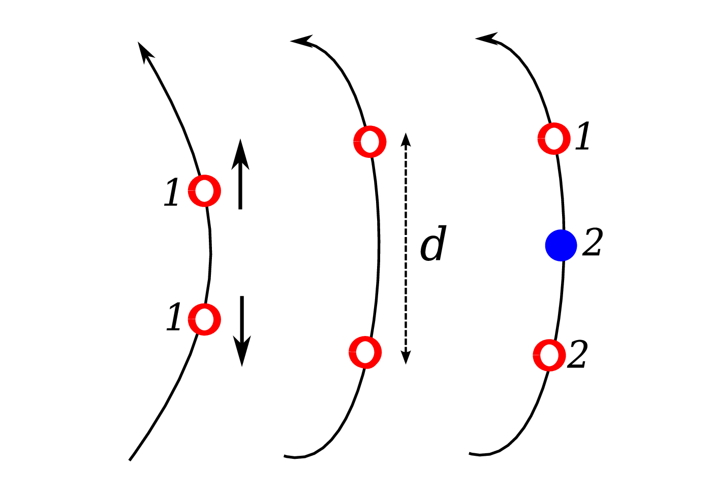
We model the magnetic field by considering the evolution of thin flux tubes, frozen into a flow, each with constant magnetic flux . We first focus on the kinematic behaviour, where the velocity field is independent of magnetic field. Later we shall introduce the Lorentz force into the system to account for the back reaction of the magnetic field on the velocity field. To ensure that , we require that our flux tubes always take the form of closed loops. Numerically, we disctretize the loops into fluid particles and track their positions and relative order (i.e., magnetic field direction) by introducing a flag , whose value increases along a given magnetic flux tube. Initially the particles are set a small distance apart, , where is a certain (small) constant length scale. If, during the evolution of the loops, the distance between two neighbouring fluid particles on a loop becomes larger than , we introduce a new particle between them, as illustrated in Fig. 2. We use linear interpolation to place the new particle halfway between the old ones. For example if inserting a new particle between particles and the position of the new particle is given by,
| (2) |
The separation between the new particles is thus greater than – a feature which will be important when we consider removing particles. The effective spatial resolution of our model is thus close to . We shall discuss later a prescription for which is more accurate than Eq. (2).
Each particle is also assigned a flag which denotes the strength of the magnetic field at that position on the loop. Assuming magnetic flux conservation and incompressibility, the magnetic field strength in the flux tube is proportional to its length. Initially the magnetic field is constant at all particles in each loop, . However, when a new particle is introduced, the magnetic field is doubled at certain particles, as shown in Fig. 2. Importantly, the field strength is increased at two out of three particles involved: this prescription emerged from our experimentation with various schemes, and allows us to reproduce the evolution of magnetic field strength in a shear flow. Conversely, when the flow reduces the separation of particles to less than , we remove a particle. The value of the magnetic field strength flag is also halved on the remaining particles in a manner consistent with the above algorithm. We have verified that this prescription reproduces accurately an exact solution of the induction equation for a simple shear flow.
Results presented below have been obtained with a typical number of trace particles of order .


II.1 Shear flow test
In order to test our model we consider a two dimensional shear flow with a Gaussian profile,
| (3) |
and a flux tube extended across the flow from to . For , Eq. (1) can easily be solved exactly to yield,
| (4) |
where is the initial field strength. Since,
| (5) |
where is the magnetic flux and is the length of the flux tube, and since is independent of , we have
| (6) |
We find excellent agreement between Eq. (6) and our numerical solution. In Fig. 3 we plot at a fixed value of versus time to compare it with Eq. (4). The comparison is quite satisfactory; the step-wise change in the numerical solution for arises because, in this simple flow with a the shear rate slowly varying in space, many new trace particles are introduced simultaneously as the flux tube is stretched, and then no particles are added for some time until the next series of particle insertions. After , we reverse the flow to observe that the particles and magnetic field return to their initial states, to demonstrate that our algorithm correctly describes the contraction of the flux tubes as well. Fig. 4 shows that the flux tube adopts the shape of the flow before the flow field is reversed, colour coding indicating the magnetic field strength.
II.2 Reconnections
Reconnections are introduced into the model in a straightforward manner. If the separation between two particles, which are not neighbours, becomes less than a certain scale , we reconnect their associated flux tubes by reassigning the flags which identify the particles ahead and behind those involved in the reconnection, as shown in Fig. 5. We found that has to be comparable to the separation of the trace particles, , in order to obtain meaningful numerical results, e.g., . Two particles are removed from the system after each reconnection event, those labelled and in Fig. 5, and their magnetic energy is lost, presumably to heat. We also monitor the cross product of the tube tangent vectors close to the reconnection point. By ensuring that the magnitude of the cross product is smaller than some tolerance and that the magnetic fields in the reconnecting loops are (almost) oppositely directed, we prevent parallel flux tubes from reconnecting. In Fig. 6 we show snapshots from a simulation before and after two simultaneous reconnection events. Since we monitor the amount of magnetic energy released in each reconnection event, we know the total magnetic energy released by the reconnections over any given time period. Finally we introduce a minimum loop size of , i.e., no magnetic loop can contain less than three particles. Any smaller loop is removed from the system, releasing its energy. We shall see later that this cutoff is important when we take derivatives along the loops to calculate magnetic tension.
II.3 Flux expulsion
We test the reconnection algorithm by considering magnetic flux expulsion from a region with closed streamlines [17]. Consider an initially uniform magnetic field , in our case a single flux tube extended over along . Differential rotation is applied to the field, with velocity given in cylindrical polar coordinates by
| (7) |
Solutions of the induction equation grow linearly in time until a maximum magnetic field is achieved,
| (8) |
where is the magnetic Reynolds number, after which magnetic diffusion destroys the field in the rotating region. We find a similar scaling of the maximum magnetic field strength, with the dimensionless quantity
| (9) |
which we identify as the effective magnetic Reynolds number. Here and are typical velocity and length scales respectively, is the reconnection length, and is the characteristic reconnection speed. In the case of the Gaussian vortex this is taken as the relative velocity of the approaching flux tube. Figure 7 shows snapshots of a typical simulation as it proceeds: the magnetic field after one winding (), in a state close to the maximum field strength (), as the reconnections start to drive the destruction of the field (), and finally the quasi-steady state (). The first plot in Fig. 8 shows the corresponding values of versus time; the linear growth before the onset of reconnections is apparent. The second plot in Fig. 8 shows the power-law relationship between and : the slope of the fit shown is , in a reasonable agreement with Eq. (8). One final test, results not presented here, was to ensure that no dynamo could be supported by driving the flux ropes with a two dimensional flow, i. e. .


III Model of a turbulent flow
Our next step is to choose the velocity field which drives the dynamo. Following previous work [28], to bypass the computational limitations of direct numerical simulations (DNS), we use the so-called Kinematic Simulation (KS) model. The KS model has primarily been used as a Lagrangian model of turbulence and results are in good agreement with DNS [9, 16, 18]. This flow is known to be a hydromagnetic dynamo [28]. The KS model prescribes the flow velocity at a position and time through the summation of Fourier modes with randomly chosen parameters (which are then kept fixed), according to [18]:
| (10) |
where , is the number of modes, and are their wave vectors and frequencies (see [28] for details). The unit vectors are chosen randomly, and where is the wave number of the ’th mode. We choose the directions of , and randomly, imposing only orthogonality with , which gives
| (11) |
and likewise for . We then select a kinetic energy spectrum and set
| (12) |
This ensures that
| (13) |
One of the main advantages of the KS model is that we have complete control of the energy spectrum, via appropriate choice of and . We also note that by construction. We adopt a modification of the von Kármán spectrum,
| (14) |
which reduces to in the inertial range, , with at the integral scale; produces the Kolmogorov spectrum, and is the cut-off scale. Figure 9 shows the energy spectrum of the KS flow, obtained numerically after fast Fourier transforming calculated from Eq. (10) on a mesh. We also show a slice, in the -plane, of the corresponding vorticity field.
The results presented below have been obtained with and , so that the smallest velocity scale is . For comparison, the reconnection scale is adopted as unless stated otherwise. With this prescription, the effective magnetic Prandtl number in our model is larger than unity.

To check if our results depend on the form of the flow, we also use an ABC flow of the form [7],
| (15) |
known as the 111 ABC flow. Dynamo action driven by ABC flows has been studied extensively [10]. This particular flow has eight stagnation points for . In the plane in which the flow converges to a particular stagnation point, the magnetic field is advected, and becomes elongated in the direction of the streamlines which diverge from the stagnation point. The resulting magnetic structures are commonly described as ‘magnetic flux cigars’ [8]. Figure 10 shows such magnetic structures produced by our numerical solution of the induction equation, along with the corresponding velocity field.
IV Diffusive and reconnection-based dynamos
Comparisons of the solution of the induction equation with those produced by the flux rope model are not straightforward because of the difference in the control parameters of the two models: the magnetic Reynolds number and the reconnection length , respectively. Following the previous section, we introduce the effective magnetic Reynolds number as , where is the characteristic reconnection speed.
We find that the dynamo based on reconnections is more efficient than the diffusion-based dynamo, in the sense that the growth rate of magnetic field of the former is significantly larger when . Therefore, in order to achieve conservative conclusions, we compare dynamos with similar growth rates of magnetic field. Thus, we have in the models which we compare.

An advantageous property of both KS and ABC flows is their analytic nature, which means that we can follow (Lagrange-like) fluid particles in the flow without using an Eularian mesh. The initial condition of our simulations is an ensemble of random closed magnetic loops; both the induction equation and the flux rope model are evolved with the same velocity field (apart from the overall normalisation to provide comparable growth rates of magnetic field). The initial condition for the induction equation is obtained by Gaussian smoothing of the magnetic field in the ropes, where we define the smoothed field , as
| (16) |
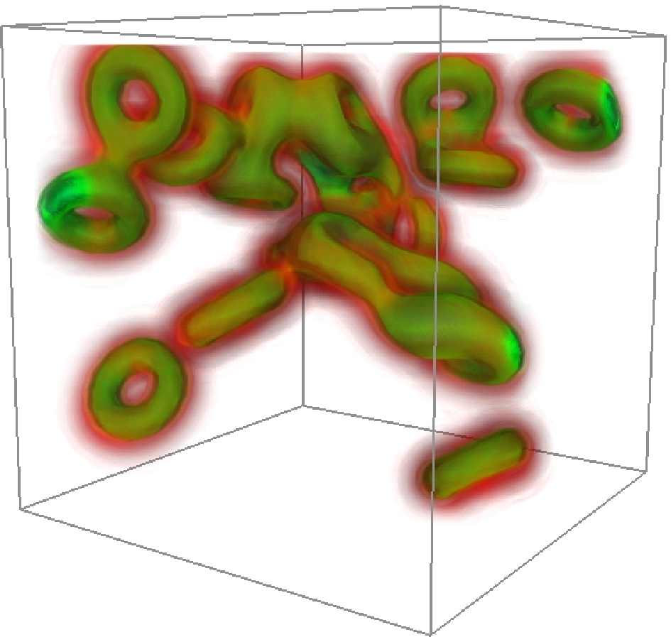
Importantly, this procedure preserves the solenoidality of the field, i. e., . Figure 11 shows the smoothed initial magnetic field used in a typical simulation, along with the corresponding flux rope setup.
The induction equation is solved using the Pencil Code [4], which implements a high-order finite-difference scheme, on a mesh with in a periodic box. Simulations with the KS velocity field had , , and ; here is based on the largest velocity scale . In a separate simulation flux ropes are advected and stretched by the same velocity field, where the positions of the trace particles are evolved using a order Runge–Kutta scheme, with a time step of . The algorithm for inserting and removing particles is applied every time step, and the reconnection algorithm, every ten time steps. We choose to be 1/4 of the smallest length scale in the flow and set , where is the reconnection length scale.


In Fig. 12 we present snapshots of the magnetic field from the flux rope simulations, driven by the KS flow, as it evolves, Fig. 13 shows the corresponding evolution in the ABC flow. In the case of the ABC flow, one notices an anticorrelation between the curvature of the flux tube and the magnetic field strength (colour coded) as suggested by Schekochihin et al. [22].
Our model is deliberately oversimplified with respect to the (incompletely understood) physics of magnetic reconnections. Nevertheless, we can argue that our model is conservative with respect to the reconnection efficiency. The reconnecting segments of magnetic lines in our model approach each other at a speed for the Kolmogorov spectrum, equal to velocity at the small scale with the energy-range scale of the flow and assumed to be close to the turbulent cut-off scale. If the magnetic field is strong enough, the Alfvén speed , which controls magnetic reconnection in more realistic models, is of order . Then and our model is likely to underestimate the efficiency of reconnections. The Sweet–Parker reconnection proceeds at a speed of order , whereas the Petschek reconnection speed is comparable to [20]. For and , the reconnection rate in our model is larger than the former but much smaller than the latter.
V Coupling with the Navier–Stokes equation and dynamo saturation
A remarkable feature of the model of reconnecting magnetic flux tubes suggested here is that is admits straightforward extension to include the back-reaction of magnetic field on the flow via the Lorentz force. Such a generalisation is presented in this section. To obtain a flow similar to the KS flow (10) as a solution of the Navier–Stokes equation, we include a driving force shown here after the viscous term:
| (17) |
where is the convective (Lagrangian) derivative, Re is the Reynolds number, is the KS velocity field (10), and is a certain relaxation time. The smaller is , the closer is to the KS flow. Since we assume that magnetic field is localised within flux ropes, magnetic pressure must be balanced by some other force, presumably by gas pressure, so we assume that , and only the magnetic tension force remains to be balanced in the Navier–Stokes equation. Neglecting viscosity, , we then obtain
| (18) |
If magnetic field is confined into thin ropes and aligned with their axes, magnetic tension involves the directional derivative of magnetic field along the rope axis alone, , where is the distance measured along the rope. Thus, it is sufficient to have magnetic field defined on magnetic loops (rather than at any position in the volume) in order to calculate magnetic tension force.
We require a solution of Eq. (18) at the changing positions of the trace particles, so we need, essentially, a Lagrangian solution of this equation. Assuming that the flow is close to the relaxed state and does not change rapidly, we put to obtain the trace particle velocities as
| (19) |
This approximation filters out rapid wave motions, e.g., Alfvén waves, which simplifies numerical simulations. We use this approximation to study the saturation of the dynamo action in Section V.1, where we consider rather long time intervals.
On the other hand, our model also allows us to include Alfvén waves and their nonlinear interactions. For this purpose we assume that and the Navier–Stokes (or rather Euler) equation reduces to
| (20) |
which, can be coupled with the equation for a frozen-in magnetic field , written in a similar form:
| (21) |
Imposing a homogeneous magnetic field and a weak perturbation, and linearising these equations leads to the wave equation describing the Alfvén waves. Since we assume that magnetic pressure is precisely balanced by gas pressure, our model does not admit compressible waves.
The nonlinearity requires that we make two changes to our numerical calculations. Firstly in our model is only defined at positions on the magnetic line (flux tube), and so the velocity field can only be evolved at those positions. The fourth-order Runge–Kutta time stepping scheme used in the kinematic regime is not suitable as it requires velocity field at positions where magnetic field is not defined. Therefore, we use the three-step Adams–Bashforth scheme instead to evolve the positions of the trace particles:
where is the size of the timestep.
The differentiation of the magnetic field along the flux tubes requires an improved accuracy for the positions of newly introduced trace particles in a stretched flux tube. A first-order prescription (2) is no longer accurate enough and we replace it by a second-order interpolation scheme. Consider a section of magnetic line traced by three particles at positions , and . If the distance between and becomes greater than , we introduce a new particle at the position given by
where is a parameter. For , the new particle is placed between and as required. In tests, in particular with Alfvén waves, we found a substantial improvement in the accuracy of the solution with this higher-order scheme. However kinematic results show no quantifiable difference between the two schemes.

The directional derivative of magnetic field has to be calculated carefully in our case since the separation of trace particles is not constant. We use the following numerical schemes to evaluate the first derivative:
| (22) |
where the notation is defined in Fig. 14, with replacing . For , we recover a commonly used finite difference scheme.
V.1 Saturated dynamos
Our starting point here is Eq. (19) for the velocity field. At each position on a flux tube, , we calculate the KS velocity field using Eq. (10), and modify it with magnetic tension force. The directional derivative of magnetic field along the tube, , is computed using Eq. (22).
The details of the simulations are similar to those in the kinematic regime. We find our timestep of to be sufficient to capture the dynamics of the motion (we found no noticeable difference between simulations with the timestep set an order of magnitude smaller than this). The relaxation time is set to be the same as the timestep, .

Figure 15 shows the r.m.s. magnetic field strength as a function of time, where the initial exponential growth is followed, at , by the saturation of the dynamo action, with fluctuating around a roughly constant level.


Snapshots of the magnetic ropes shown in Fig. 16 illustrate the spatial evolution of the magnetised region. Unlike virtually all earlier simulations of the fluctuation dynamo, most often performed in periodic boxes with volume-filling initial conditions, the initial magnetic field in our simulations is localised in space, as shown in the upper left panel of Fig. 16 (which refers to an early stage of evolution). In the kinematic stage, , magnetic field growth is accompanied by the spread of the magnetised region clearly visible in the first three snapshots. Consistently with the action of magnetic diffusion , the size of the region occupied by magnetic ropes grows at However, the spread is halted in the nonlinear, saturated stage represented in Fig. 16 by snapshots at and , which suggests that the turbulent magnetic diffusivity is suppressed in the saturated state. This appears to be a result of the suppression, by magnetic tension, of random stretching of magnetic field at the location of a flux rope. In other words, the saturation of the dynamo action is achieved via the suppression of the effective magnetic Reynolds number, , where is the effective microscopic magnetic diffusivity. This idea is fully consistent with the arguments of Subramanian [26] who considered a similar nonlinearity in the Kazantsev model of the fluctuation dynamo [13, 14, 27, see also] and also of Schekochihin et al. [23], Schekochihin et al. [24] who suggested a simple model of the effect of Lorentz force. A general feature of these models is that the small-scale dynamo saturates because of a ‘renormalization’ of the coefficients governing its evolution, and the corresponding decrease in the effective magnetic Reynolds number. This can be the result of enhanced nonlinear diffusion [26], increased diffusion together with additional hyperdiffusion [27], or reduced stretching [13, 14, 23, 24]. Our model is consistent with the saturation of the dynamo action via the suppression of the magnetic Reynolds number, now arising from a reduction of localised random stretching, or turbulent magnetic diffusivity.

To clarify further the mechanism of dynamo saturation, we monitored the average separation of trace particles in the flow. At the start of a simulation each trace particle located on a magnetic loop is assigned a neighbour, for convenience the particle next to it. As the simulation proceeds, the particles are advected by the flow, and new particles may be introduced between them, but we continue to monitor the separation between the original pair of particles. The particle separation averaged over all the original particle pairs, , is shown in Fig. 17. Indeed, the separation of the particles stops growing as soon as the dynamo enters the nonlinear stage. We stress that, at late times, not all pairs of trace particles belong to the same magnetic loop because of multiple reconnections that often split a magnetic loop into smaller ones. Thus, the fact that ceases to grow implies that not only stretching is suppressed within a single loop, but also that the magnetic loops stop spreading in space.

We performed another experiment, where the location of the test particles used to compute the dispersive properties of the flow was not restricted to the magnetic loops. To reduce technical problems, we considered two time-independent flows obtained as the snapshots of the original KS velocity field and of its form affected by magnetic tension force at a certain moment in the saturated dynamo state. The evolution of the particle separation (averaged over 500 pairs) is shown in Fig. 18, where one can distinguish the initial exponential growth of the separation, followed by the Richardson regime when , and then by the incoherent, diffusive dispersion at larger separations. However, the separation of the particles is insensitive to the effects of the Lorentz force: the two curves in Fig. 18 hardly differ from each other. Thus, the flow has not been strongly affected by the Lorentz force, except for the close vicinity of the flux tubes.
Importantly, the mean particle separation is a measure of kinetic turbulent diffusivity, as opposed to the magnetic one. The former involves the mean square of the total velocity , whereas the turbulent magnetic diffusivity is only sensitive to the velocity field components orthogonal to the magnetic field, . Incidentally, these results imply that the turbulent magnetic Prandtl number is different from unity: in isotropic flow and magnetic field, ; the difference is small but perhaps significant in some applications. We cannot exclude that this feature is an artifact of our model where a localised modification of the velocity field by magnetic tension does not spread into a broader region as it would do due to kinematic viscosity.


V.2 Alfvén waves
To demonstrate the flexibility of the flux model suggested here, we briefly present simulations of Alfvén waves propagating along an imposed magnetic field. For this purpose we solve Eqs. (20) and (21) with a single magnetic flux tube which, initially, has constant magnetic field. The tube is perturbed as shown in the upper left panel of Fig. 19. The simulation proceeds in a box periodic in the -direction, and the interaction with the ghost wave from the next periodicity cell is seen in the final snapshot at . We confirmed that the phase speed of the wave is indeed proportional to the strength of the magnetic field. Since our model admits nonlinear interactions of Alfvén waves, it can be used to study spectral energy cascades and other features of the Alfvén wave turbulence.
VI Curvature of magnetic lines
Schekochihin et al. [22] discuss the geometry of magnetic lines in the kinematic fluctuation dynamo driven by a single-scale, -correlated in time random flow with high magnetic Prandtl number. They argue that magnetic field strength and magnetic line curvature should be anticorrelated and derive a power-law probability distribution function of the magnetic line curvature. These results are used to support the picture of folded magnetic lines as a representation of magnetic field produced by the fluctuation dynamo.
The anticorrelation between the curvature of magnetic lines and the strength of the magnetic field is intuitively appealing since magnetic field strength grows due to a random stretching of magnetic lines which is necessarily accompanied by a reduction in their local curvature. However, the stretching is not the only component of the fluctuation dynamo mechanism. In the framework of the stretch-twist-fold dynamo concept, stretching must be followed by the folding of magnetic lines to ensure an exponential growth of magnetic field – and the folding will tend to increase the local magnetic line curvature. Therefore, an anticorrrelation between magnetic curvature and strength may be expected for a decaying magnetic field rather than for magnetic fields growing due to the dynamo action. In this section we explore directly the relation between the magnetic line curvature and strength using the reconnecting flux rope dynamo model.
The curvature of the flux ropes can be calculated as [11]
| (23) |
where is a parametrised space curve representing a magnetic flux rope, with the distance measured along the rope, and dash denotes derivative with respect to , with the first derivative calculated using Eqs. (22) and the second derivative, from
| (24) |
where notation is defined in Fig. 14. For , this form reduces to a standard finite difference scheme.

Figure 20 is the scatter plot of magnetic field strength at a particular position versus the field line curvature at that point, computed at the end of the simulation, illustrated in Fig. 12, where the dynamo is driven by the KS flow. Only the envelope of the curvature distribution appears to be consistent with the anticorrelation, and even that only for relatively strong fields, . Thus, the range of the curvature values is narrower at positions where the field is stronger, but for any field strength this range includes very small curvature values.
Those parts of magnetic flux tubes where magnetic field is weak have low curvature, especially those with with the initial field strength ( at the particular time of the simulation). In our model, the only way the field strength can become smaller than is through the shrinking of a flux tube caused by contracting flow. In a perfectly conducting fluid, such a contraction can make the curvature larger, e.g., when a wavy magnetic line is contracted along its wave vector. However, the situation changes entirely in the presence of reconnections (or any other magnetic dissipation mechanism): now, reconnections eventually eliminate the bends of the magnetic line thus reducing the curvature of a contracting magnetic line. Apparently, we see the evidence of this in Fig. 20. The group of points with nearly maximum curvature at the top of the frame are probably those which will undergo reconnections of this type very soon. Finally we note that the reconnection length limits the maximum value that can take.

Schekochihin et al. [22] showed, both analytically and numerically, that the probability density function of the curvature of field lines has a power-law form in the limit of large . In particular, they obtain for a three-dimensional, incompressible flow. Figure 21 shows the PDF of curvature from our simulations which shows a very good agreement with the analytical results of Schekochihin et al. [25].

Schekochihin et al. [25] argue that, because the magnetic field strength is higher where the magnetic line curvature is lower (due to the stretching by velocity shear), magnetic tension force (which is quadratic in ) is lower at positions with weak field. This conclusion relies on estimating the tension force as , and noting that this quantity decreases with , although increases. This would imply that magnetic tension is relatively unimportant in regions with strong curvature. This leads these authors to a conclusion that magnetic field is organised into folded structures which persist in the saturated state. However, what matters is not the value of itself but rather its gradient along the magnetic line, . In a stretched magnetic line, the gradient is reduced in regions with strong magnetic field (i.e., the straight segments of the folded magnetic lines) and enhanced in regions of weaker field (in the turns in the folded structures). Therefore, magnetic tension will drive the turns closer to each other along each magnetic line destroying the folded structures. Thus, the lack of any apparent domination of folded structures in Fig. 12 is consistent with the curvature PDF shown in Fig. 21. We show in Fig. 22 the time variation of the slope of the curvature PDF into the nonlinear regime (discussed in Section V): the PDF becomes steeper , so that high curvature occurs less often in the nonlinear state. This can be attributed to magnetic tension which tends to reduce magnetic line curvature.
VII Statistics of magnetic energy release
Solar corona is one of the astrophysical environments where magnetic reconnections are believed to play important role, particularly in heating the plasma to the high temperatures observed [20]. The reconnections are assumed to be driven by the motion of the footpoints of magnetic flux tubes anchored in the photosphere and extending into the corona [21, and references therein]. Reconnection events that release large amounts of magnetic energy are observed as solar flares. A remarkable feature of the coronal heating mechanism is that the frequency distribution of the flare energy has a power law form in a very broad energy range (eight orders of magnitude) [6, see an excellent review of]
| (25) |
If , most of the magnetic energy released into the corona is due to weak flares. This attractive option suggested by Parker [19] is known as the nanoflare model of the coronal heating. This idea is most often explored in the context of self-organised criticality models based on cellular automata, which are known to demonstrate the required power-law statistical distributions. Notably, the continuous analogies of these models involve the hyperdiffusion operator [6]. A widely recognised difficulty of this approach is the elusive connection with the physical picture and even unclear physical interpretation of the variables. Alternative models [12, e.g.,], where reconnection evens are modelled directly, also reproduce the power-law statistics, but still remain rather idealised regarding the behaviour of magnetic flux tubes.
Our model is quite different from the Solar corona settings, where the reconnections are driven by the motion of the flux rope footpoints, the plasma is believed to be magnetically dominated, and in situ dynamo action is improbable. Nevertheless, in this section we consider the statistics of the energy release in our model of the flux rope dynamo. As we show here, our reconnection dynamo model naturally develops a power-law distribution (25) with , which appears to be independent of the form of the velocity field. Our model can readily be adapted to the Solar corona conditions, and despite the differences of our model from the Solar corona models, we feel that this feature of the model can be relevant in this context.
In the case of the induction equation, the magnetic energy dissipation rate can be defined as
| (26) |
where is the total magnetic energy. A similar quantity can be obtained for the flux rope dynamo by summing the contributions of all reconnection events to the magnetic energy release:
| (27) |
where is a suitable time interval during which reconnections occur (we take to be equal to ten time steps; individual reconnection events occur in a single time step), and , and are the magnetic field strength, the cross-sectional area and length of the reconnected (and thus removed) flux tube segment associated with a trace particle number . From our assumption of frozen flux , the total magnetic energy is,
| (28) |
where is the total number of trace particles in all flux tubes. Thus,
| (29) |


In Fig. 23 we present the energy release rates in simulations where the growth rate of the magnetic field is in both simulations (with the unit time ). The dashed line shows the energy release rate from a simulation of induction equation with , which has the mean energy release rate . The solid line shows the corresponding results from the reconnection dynamo, with the mean value plotted as a thick horizontal line. The mean value of the energy release rate from the reconnecting flux rope dynamo is , an order of magnitude larger than that obtained from the induction equation. We also note the strong fluctuations in the energy release rate from the reconnection model, as opposed to the quiescent behaviour in the induction equation. It is important that an order of magnitude difference in the energy release rates occurs in solutions with similar growth rates of magnetic field. Since the reconnection based dynamo is more efficient than that based on magnetic diffusion (see section IV) kinetic energy density in the former being 10 times smaller than in the latter. With comparable kinetic energy densities, the difference between the energy release rates can be even larger.
As shown in Fig. 24, dynamos driven by the ABC flow behave similarly. With , the induction equation gives an energy release rate of about . The corresponding flux rope dynamo with the same growth rate () has energy release rate , again ten times larger.


We show in Figs. 25 and 26 the probability distributions of the magnetic energy release rate, normalised to the total magnetic energy in the domain, , with or . Here overbar denotes time averaging (at times where an eigensolution has been established) and is the standard deviation of . Since , it can easily be seen that . We obtained the probability distributions of from both the induction equation and the reconnection dynamo model, both driven by the KS flow, shown in Fig. 25, and also with both based on the 111 ABC flow, shown in Fig. 26. The power-law index obtained for the KS flow is , and that for the ABC flow is . We stress that this power-law behaviour is not related to the nature of the velocity field: solutions of the induction equation with the same velocity fields, as we show in Fig. 25, exhibit an approximately Gaussian probability distribution.
Results shown in Figs. 25 and 26 have been obtained from kinematic simulations, where the velocity field was not affected by the Lorentz force. However, the corresponding nonlinear model introduced in Section V retains this feature, with for the KS flow in the statistically steady state, as we show in Fig. 27.
It is not quite clear if the flux rope dynamo represents a physical example of self-organised criticality, but the system seems to possess at least some of the required properties. In particular, as we argue above, our model can be viewed as an extreme case of magnetic hyperdiffusivity, which also arises in the self-organised criticality models of Solar flares.
VIII Discussion and conclusions
To summarise, we have confirmed that the dynamo action is sensitive to the nature of magnetic dissipation and demonstrated that magnetic reconnections (as opposed to magnetic diffusion) can significantly enhance the dynamo action. We have explored the kinematic stage of the fluctuation dynamo in a chaotic flow that models hydrodynamic turbulence and in the ABC flow, with the only magnetic dissipation mechanism being the reconnection of magnetic lines implemented in a direct manner. In our model, where magnetic dissipation is suppressed at all scales exceeding a certain scale , the growth rate of magnetic field exceeds that of the magnetic diffusion-based fluctuation dynamo with the same velocity field. Even when the velocity field of the reconnection-based dynamo is reduced in magnitude as to achieve similar growth rates of magnetic energy density, the rate of conversion of magnetic energy into heat in the reconnection dynamo is an order of magnitude larger than in the corresponding diffusion-based dynamo. Thus, reconnections more efficiently convert the kinetic energy of the plasma flow into heat, in our case with the mediation of the dynamo action. This result, here obtained for a kinematic dynamo, can have serious implications for the heating of rarefied, hot plasmas where magnetic reconnections dominate over magnetic diffusion (such as the corona of the Sun and star, galaxies and accretion discs).
It is intriguing that reconnections play the same role [15, 2] of converting kinetic energy into heat in superfluids and Bose-Einstein condensates, fluids near absolute zero at the opposite end of the temperature spectrum.
Our model can be viewed as a numerical implementation of the elusive limiting regime of infinitely large magnetic Reynolds number, where magnetic dissipation can be safely neglected at all large scales but plays a crucial role at a certain very small scale (we are grateful to Alex Schekochihin for suggesting this idea).
In contrast to the fluctuation dynamo based on magnetic diffusion, the probability distribution function of the energy released in the flux rope dynamo has a power law form not dissimilar to that observed for the Solar flares. This is also true for the nonlinear states of the dynamo.
The reconnection-based dynamo model suggested here can be generalised to include the modification of the velocity field by the Lorentz force. More precisely, magnetic pressure is assumed to be balanced by the gas pressure, so that only magnetic tension needs to be explicitly included into the Navier–Stokes equation. Magnetic tension can readily be calculated in our model where magnetic field is defined only at discrete positions of closed magnetic loops. We suggest two approximations for the Navier–Stokes equation, one designed to model Alfvén waves and the other suitable for the studies of nonlinear dynamos. The former model can be useful in the studies of nonlinear interaction of Alfvén waves and Alfvénic turbulence.
Unlike most – if not all – other simulations of the fluctuation dynamo, our computations start with a spatially localised initial magnetic field. This has allowed us to observe that the magnetised region spreads during the kinematic dynamo stage but its size stops growing in the nonlinear stage. This can be naturally interpreted as the suppression of the turbulent magnetic diffusion in the saturated dynamo state. This is broadly equivalent to the reduction of the effective magnetic Reynolds number down to its marginal value (with respect to the dynamo action).
Our model of magnetic field evolution, based on tracing closed magnetic loops can be fruitfully applied in other numerical approaches to magnetohydrodynamics. One of well-known difficulties in the generalisation of smoothed-particle hydrodynamics to include magnetic fields is the implementation of the solenoidality of magnetic field. Quite notably, our approach satisfies the magnetic solenoidality condition perfectly since the modelled magnetic lines are closed at all times. A similar approach may be fruitful in smoothed-particle magnetohydrodynamics codes.
Acknowledgements
We thank Pat Diamond, Russell Kulsrud, Alex Schekochihin, Andrew Soward for useful discussions. This work was supported by the STFC grant ST/F003080/1. AS is grateful to IUCAA for financial support and hospitality.
References
- [1] Baggaley, A. W., Barenghi, C. F., Shukurov, A., and Subramanian, K.: 2009, ArXiv e-prints
- [2] Barenghi, C. F.: 2008, Physica D Nonlinear Phenomena 237, 2195
- [3] Blackman, E. G.: 1996, Phys. Rev. Lett. 77, 2694
- [4] Brandenburg, A.: 2002, Comp. Phys. Comm. 147, 471
- [5] Brandenburg, A. and Sarson, G. R.: 2002, Phys. Rev. Lett. 88(5), 055003
- [6] Charbonneau, P., McIntosh, S. W., Liu, H.-L., and Bogdan, T. J.: 2001, Solar Phys. 203, 321
- [7] Childress, S. and Gilbert, A.: 1995, Stretch, Twist, Fold: The Fast Dynamo, Springer, Berlin
- [8] Dorch, S. B. F.: 2000, astro-ph/0007466
- [9] Fung, J. C. H. and Vassilicos, J. C.: 1998, Phys. Rev. E 57, 1677
- [10] Galloway, D. and Frisch, U.: 1986, Geophys. Astrophys. Fluid Dyn. 36, 53
- [11] Gray, A.: 1996, Modern Differential Geometry of Curves and Surfaces with Mathematica, CRC Press, Inc., Boca Raton, FL, USA
- [12] Hughes, D., Paczuski, M., Dendy, R. O., Helander, P., and McClements, K. G.: 2003, Phys. Rev. Lett. 90(13), 131101
- [13] Kim, E.: 1999, Phys. Lett. A 259, 232
- [14] Kim, E.: 2000, Phys. Plasmas 7, 1746
- [15] Leadbeater, M., Winiecki, T., Samuels, D. C., Barenghi, C. F., and Adams, C. S.: 2001, Physical Review Letters 86, 1410
- [16] Malik, A. and Vassilicos, J.: 1999, Phys. Fluids 11, 1572
- [17] Moffatt, H. K.: 1978, Magnetic Field Generation in Electrically Conducting Fluids, Cambridge Univ. Press
- [18] Osborne, D., Vassilicos, J., Sung, K., and Haigh, J.: 2006, Phys. Rev. E 74, 036309
- [19] Parker, E. N.: 1983, Astrophys. J. 264, 642
- [20] Priest, E. and Forbes, T.: 2000, Magnetic Reconnection, Cambridge University Press
- [21] Priest, E. R., Longcope, D. W., and Titov, V. S.: 2003, Astrophys. J. 598, 667
- [22] Schekochihin, A., Cowley, S., Maron, J., and Malyshkin, L.: 2002a, Phys. Rev. E 65(1), 016305
- [23] Schekochihin, A. A., Cowley, S. C., Hammett, G. W., Maron, J. L., and McWilliams, J. C.: 2002b, New J. Phys. 4, 84
- [24] Schekochihin, A. A., Cowley, S. C., Taylor, S. F., Hammett, G. W., Maron, J. L., and McWilliams, J. C.: 2004, Phys. Rev. Lett. 92(8), 084504
- [25] Schekochihin, A. A., Maron, J. L., Cowley, S. C., and McWilliams, J. C.: 2002c, ApJ 576, 806
- [26] Subramanian, K.: 1999, Phys. Rev. Lett. 83, 2957
- [27] Subramanian, K.: 2003, Phys. Rev. Lett. 90(24), 245003
- [28] Wilkin, S. L., Barenghi, C. F., and Shukurov, A.: 2007, Phys. Rev. Lett. 99, 134501