Solvable Model of Spiral Wave Chimeras
Abstract
Spiral waves are ubiquitous in two-dimensional systems of chemical or biological oscillators coupled locally by diffusion. At the center of such spirals is a phase singularity, a topological defect where the oscillator amplitude drops to zero. But if the coupling is nonlocal, a new kind of spiral can occur, with a circular core consisting of desynchronized oscillators running at full amplitude. Here we provide the first analytical description of such a spiral wave chimera, and use perturbation theory to calculate its rotation speed and the size of its incoherent core.
Keywords:
chimera states, Kuramoto model, nonlocal coupling, spiral waves, reaction-diffusion systempacs
05.45.Xt, 05.65.+bLarge systems of coupled limit-cycle oscillators have been used to model diverse phenomena in physics, chemistry, and biology [1, 2]. Examples range from spiral waves in heart muscle [3] and brain tissue [4], to synchronization of nerve cells [5], pendulums [6], fireflies [7], and Josephson junctions [8].
Most of the early theoretical work on these systems assumed either local coupling (through nearest-neighbor or diffusive interactions) or global coupling (through infinite-range interactions, corresponding to a mean-field approximation). In the past few years, however, several researchers have begun to explore other types of connectivity. One line of research investigates what happens if the coupling is neither local nor global but somewhere in between, as occurs naturally in certain neural, chemical, and biochemical systems [9, 10, 11, 12].
Around 2002, Kuramoto and his colleagues discovered a spatiotemporal pattern that appears to be unique to such nonlocally coupled systems [10, 11]. They showed numerically that systems of identical oscillators with symmetrical coupling could self-organize into a state in which some oscillators were mutually synchronized while others remained desynchronized. An exact solution for this “chimera state” was later obtained for phase oscillators arranged on a ring [13, 14], and its dynamics and bifurcations were further clarified by studying two interacting populations of oscillators [15, 16, 17].
The most surprising result emerged from simulations of two-dimensional arrays [18, 19, 20]. Kuramoto and coworkers [20, 18, 21] showed that two-dimensional chimeras are spiral waves with a phase-randomized core of desynchronized oscillators surrounded by phase-locked oscillators in the spiral arms. Nothing like this had ever been seen before; in ordinary reaction-diffusion systems, the smoothing effects of diffusion would prevent the spatial discontinuities implied by an incoherent core.
In this Letter we present the first analytical solution for a spiral wave chimera. Our analysis predicts the existence of the incoherent core and yields a simple formula for its radius as well as for the rotation rate of the spiral arms.
The model we consider is
| (1) |
where is the phase of the oscillator at position at time , is its natural frequency, and is a phase lag. The kernel is a normalized Gaussian:
| (2) |
Note that the width of determines a length scale for the system. Varying can be thought of as choosing different first harmonics of a general coupling function [22]. In contrast, is dynamically irrelevant, and can be set to zero without loss of generality.

Figure 1(a) shows a spiral wave chimera for Eqs. (1), (2), computed numerically. Notice the phase-randomized core at its center, as highlighted in Fig. 1(b). The spatial structure of this pattern is governed by an integral equation, originally derived by Shima and Kuramoto [18] via the following self-consistency argument. Define a local mean field (a complex order parameter) by
| (3) |
so that (1) can be rewritten as
| (4) |
Now seek statistically steady solutions of Eqs. (1), (2). For this special class of solutions we can find a rotating coordinate frame (in state space, not physical space) in which the phase-locked oscillators in the spiral arms appear motionless, and the mean field becomes stationary across the entire pattern [19, 18]. To define this rotating frame, let and where is as yet unknown. Then using (3) and (4) we find
| (5) |
where the time-independent mean field is given by
| (6) |
Oscillators for which will reach a steady state, , for which in Eq. (5), whereas those for which will drift but distribute themselves with a stationary density in the variable inversely proportional to their angular velocity [18, 14]. Equation (6) can then be solved self-consistently by replacing by (for locked oscillators) and by the mean of (for drifting oscillators), where the mean is calculated using the density just mentioned. The result is the nonlinear integral equation
| (7) | |||||
where . Figures 1(c) and 1(d) show and for a typical spiral wave chimera.
Our new results concern the analytical solution of Eq. (7). The first step is to simplify it using the spiral wave ansatz of Cohen et al. [23]. Considering the appearance of the functions and in Figs. 1(c) and (d), it is natural to use the ansatz and , where are polar coordinates. Substituting this into (7) one obtains
| (8) | |||||
where
| (9) | |||||
and is the modified Bessel function of the first kind of order . This ansatz has replaced the problem of finding the functions of two variables, and , by that of finding and , both functions of a single variable.
Nevertheless, solving Eq. (8) is still a formidable task. To make progress, we use perturbation theory to analyze (8) in the limit of small . First observe that at , Eq. (1) is a gradient system in a coordinate frame rotating at speed ; hence, in this frame all the attractors for (1) must be fixed points. Back in the original frame, these fixed points correspond to phase-locked states rotating at frequency . Therefore when [14], which motivates the series expansions
| (10a) | |||||
| (10b) | |||||
| (10c) | |||||
as . Substituting (10a)-(10c) into (8) we obtain, to lowest order,
| (11) |
Hence
| (12) | |||||
and
| (13) |
Equation (12) shows that at leading order, the amplitude of the mean field increases with and satisfies and , in agreement with the behavior seen when (Fig. 1(d)). Furthermore, under the physically reasonable assumption that can be written as a power series in , one can show that is the only solution of (13); then, from the rotational invariance of the problem we can set . This result indicates that the spiral arms approach radial straight lines as , a fact we have also confirmed numerically.
At we obtain and
which, after defining , yields an inhomogeneous Fredholm equation of the second kind:
| (14) |
We have been unable to solve (14) analytically, but extensive numerical investigations suggest that to satisfy (which we know to be true, given that ), must be very close to 1. To show that this is plausible we note that for ,
| (15) |
so that if is slowly varying near , the left side of (14) is approximately zero while the right side of (14) is approximately .
Recalling that it is those oscillators with which drift, we can see that to order the radius of the incoherent core is , where . In the limit as , , and hence, using , we have
| (16) |
Thus, to order we have two testable predictions regarding the behavior of the spiral wave chimera as :
- 1.
Spiral arms rotate at angular velocity .
- 2.
Incoherent core radius is given by .
Figure 2 shows measurements of both and the radius of the incoherent core from a simulation of Eq. (1), as is varied. The data points agree very well with the above predictions, despite the use of a finite domain.


Along with testing our analytical results against simulations, we have also tested them against numerical solutions of the integral equation (8). The results for a domain are shown in Fig. 3 as is varied. Figure 3(a) compares , the only non-trivial zeroth order term in our series expansion, to the computed obtained for two different values of . Boundary effects near are clearly visible. For , is indistinguishable from for . Figure 3(b) plots for three different values of ; this choice of dependent variable is motivated by Eq. (10c), which predicts that should be proportional to , for small. Figures 3(c) and 3(d) show and as functions of , now found by solving (8) instead of simulating (1), in the same format as Fig. 2. The agreement with the data in Fig. 2 is excellent.
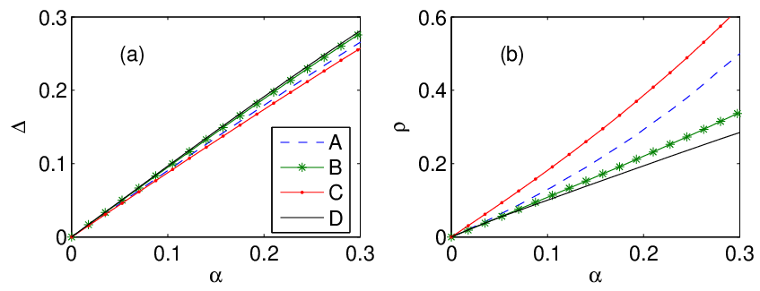
The results above were derived using the Gaussian kernel (2). In contrast, Shima and Kuramoto [18] used the modified Bessel function of the second kind, , as a kernel. This coupling function arises naturally in a class of reaction-diffusion systems where active chemical elements are indirectly coupled by passive, fast diffusive agents [18]. Using a Gaussian allowed us to explicitly perform the integral in (9) and thus make analytical progress in the subsequent perturbation analysis. For and other kernels one can evaluate the integral in (9) numerically. In Fig. 4 we show and as a function of for four different kernels, found by numerically solving (8). Interestingly, we see that while does not seem to depend on the details of the kernel, does.
Several puzzles remain about the spiral wave chimera [21]. For example, we do not understand how it bifurcates. When is increased sufficiently far from zero, the chimera becomes numerically unobservable. Perhaps, for example, it loses stability though a subcritical Hopf bifurcation, or is destroyed through a saddle-node bifurcation. Even when the chimera does exist, its core wanders erratically. This can be rationalized by observing that there is no preferred origin for the spiral in an infinite domain, so it is neutrally stable with respect to translations. The finite number of incoherent oscillators act a source of effectively random “noise” which then jiggles the spiral in these neutral directions.
A second puzzle is that the spiral wave chimera apparently exists only if is sufficiently close to 0, whereas the chimeras found in lower-dimensional systems [13, 14, 15, 16, 17] exist only if is sufficiently close to . In physical terms, two-dimensional chimeras live near the gradient system limit, whereas one- and zero-dimensional chimeras live in the opposite regime, where the dynamics have an almost reversible or conservative character. At the moment we have no explanation for this difference.
Although we have assumed identical oscillators in our analysis, this is not necessary. Spiral wave chimeras should persist in the presence of slight disorder. For example, Laing [19] studied a variant of Eq. (1) for non-identical oscillators and with a kernel which was zero for larger than a particular radius. He used the recent ansatz of Ott and Antonsen [24, 25] to derive a differential equation for a variable closely related to the order parameter. For oscillators whose intrinsic frequencies are randomly drawn from a Lorentzian distribution, the steady states of this differential equation satisfy (7), where and is the half-width-at-half-maximum of the Lorentzian distribution. The results in Fig. 2 agree qualitatively with those of Laing [19].
The possibility of observing spiral wave chimeras in physical systems naturally arises. Nonlocal coupling of the form used here occurs in some networks of neurons [9, 4], so such systems may be the best candidates. We leave the experimental observation of chimera states as a challenge to others.
Research supported in part by NSF grant CCF-0835706. We thank S. Shima for helpful advice about the simulations.
References
- [1] A. T. Winfree, The Geometry of Biological Time (Springer, New York, 1980).
- [2] A. Pikovsky, M. Rosenblum, and J. Kurths, Synchronization (Cambridge U. Press, Cambridge, U. K., 2003).
- [3] J. E. Paullet and G. B. Ermentrout, SIAM J. Appl. Math. 54, 1720 (1994).
- [4] D. Horn and I. Opher, Neural Comput. 9, 1677 (1997).
- [5] C. Chow and N. Kopell, Neural Comput. 12, 1643 (2000).
- [6] J. Pantaleone, Am. J. Phys. 70, 992 (2002).
- [7] J. Buck, Quart. Rev. Biol. 63, 265 (1988).
- [8] K. Wiesenfeld, P. Colet, and S. Strogatz, Phys. Rev. Lett. 76, 404 (1996).
- [9] C. Laing and C. Chow, Neural Comput. 13, 1473 (2001).
- [10] Y. Kuramoto and D. Battogtokh, Nonlinear Phenom. Complex Syst 5, 380 (2002).
- [11] Y. Kuramoto, in Nonlinear Dynamics and Chaos: Where do we go from here? (IOP Publishing, Bristol, UK, 2003), p. 209.
- [12] D. Tanaka and Y. Kuramoto, Phys. Rev. E 68, 026219 (2003).
- [13] D. Abrams and S. Strogatz, Phys. Rev. Lett. 93, 174102 (2004).
- [14] D. Abrams and S. Strogatz, Int. J. Bifurcat. Chaos 16, 21 (2006).
- [15] D. Abrams, R. Mirollo, S. Strogatz, and D. Wiley, Phys. Rev. Lett. 101, 084103 (2008).
- [16] A. Pikovsky and M. Rosenblum, Phys. Rev. Lett. 101, 264103 (2008).
- [17] C. R. Laing, Chaos 19, 013113 (2009a).
- [18] S. Shima and Y. Kuramoto, Phys. Rev. E 69, 036213 (2004).
- [19] C. R. Laing, Physica D 238, 1569 (2009b).
- [20] Y. Kuramoto and S. Shima, Progr. Theor. Phys. Suppl. 150, 115 (2003).
- [21] Y. Kuramoto, S. Shima, D. Battogtokh, and Y. Shiogai, Prog. Theor. Phys. Suppl. 161, 127 (2006).
- [22] T.-W. Ko and G. B. Ermentrout, Phys. Rev. E 78, 026210 (2008).
- [23] D. S. Cohen, J. C. Neu, and R. R. Rosales, SIAM J. Appl. Math. 35, 536 (1978).
- [24] E. Ott and T. M. Antonsen, Chaos 18, 037113 (2008).
- [25] E. Ott and T. M. Antonsen, Chaos 19, 023117 (2009).