zhangzz@fudan.edu.cn,sgzhou@fudan.edu.cn,jhguan@tongji.edu.cn
Average distance in a hierarchical scale-free network: an exact solution
Abstract
Various real systems simultaneously exhibit scale-free and hierarchical structure. In this paper, we study analytically average distance in a deterministic scale-free network with hierarchical organization. Using a recursive method based on the network construction, we determine explicitly the average distance, obtaining an exact expression for it, which is confirmed by extensive numerical calculations. The obtained rigorous solution shows that the average distance grows logarithmically with the network order (number of nodes in the network). We exhibit the similarity and dissimilarity in average distance between the network under consideration and some previously studied networks, including random networks and other deterministic networks. On the basis of the comparison, we argue that the logarithmic scaling of average distance with network order could be a generic feature of deterministic scale-free networks.
pacs
89.75.Hc, 89.75.Da, 02.10.Ox, 05.10.-a1 Introduction
In the last decade, a lot of authors in different scientific communities have made a concerted effort toward unveiling and understanding the generic properties of complex networked systems in nature and society [1, 2, 3, 4]. One of the most important discoveries is that despite network diversity, most real-life networks exhibit striking small-world behavior [5], that is to say, their average distance scales logarithmically with network order (number of nodes in a network), or slowly. Average distance is a fundamental measurement characterizing a complex network, which is relevant to many other structural features of the network, including degree distribution [6, 7], centrality [8], fractality [9, 10, 11], and so on. In addition, average distance has a strong effect on various dynamics running on networks, such as disease spreading [5], random walks [12], synchronization [13], amongst others. In view of its significance and usefulness, average distance has received considerable attention [14, 15, 16, 17, 18, 19, 20].
Apart from the small-world feature, a variety of real networks, particularly biological and social networks, also share two remarkable properties: scale-free behavior [21] and hierarchical structure [22, 23]. To mimic simultaneously the two prominent characteristics, Barabási, Ravasz and Vicsek proposed a deterministic model [24], hereafter called BRV model, which is the progenitor of deterministic models for complex networks and has led to an increasing number of theoretical investigations on deterministic networks that are an interesting class of networks and have been proved to be a useful tool [25, 26, 27, 28, 29, 30, 31, 32, 33, 34, 35, 36]. Many structural and dynamical properties of the BRV model have been studied in much detail, including degree distribution [24], spectra of adjacency matrix [37], random walks [38], to name but a few. However, in spite of its importance, the exact knowledge of average distance for the BRV model remains not well understood.
To fill this gap, in this paper, we study the average distance in the BRV model, the deterministic nature of which makes it possible to investigate analytically the average distance. Based on the recursive relations derived from the self-similar structure of the BRV model, we obtain the closed-form solution for the average distance. The obtained rigorous result shows that the average distance behaves logarithmically with the network order. This logarithmic scaling has also been previously reported for many other deterministic scale-free networks. We thus conjecture that the logarithmic scaling characterizes the behavior of average distance for deterministic scale-free networks.
2 The hierarchical scale-free network
Let us first introduce the BRV model, a hierarchical scale-free network that is constructed in an iterative way [24]. We denote by the BRV network model after () iterations (number of generations). Initially (), the network consists of a single root node labeled as . At the first generation (), two new nodes are added to the system and connected to the root node. Thus, we get , where node 1 is called hub node, the nodes are named bottom nodes forming a set represented as . At generation 2 (i.e., ), we generate two copies of and connect the bottom nodes of each replica to the hub of the original . The hub of the original and the four bottom nodes in the replicas become the hub and bottom nodes of , respectively. The set of the bottom nodes belonging to is denoted as . Suppose one has ; the next generation network can be obtained from by adding two copies of with their bottom nodes being linked to the hub of the original . In , its hub is the hub of the original , its bottom nodes are composed of all the bottom nodes of both copies of , and all the bottom nodes make the set . Repeat indefinitely the replication and connection steps, we obtain the hierarchical scale-free network. Figure 1 illustrates the construction process of the network for the first three iterations.
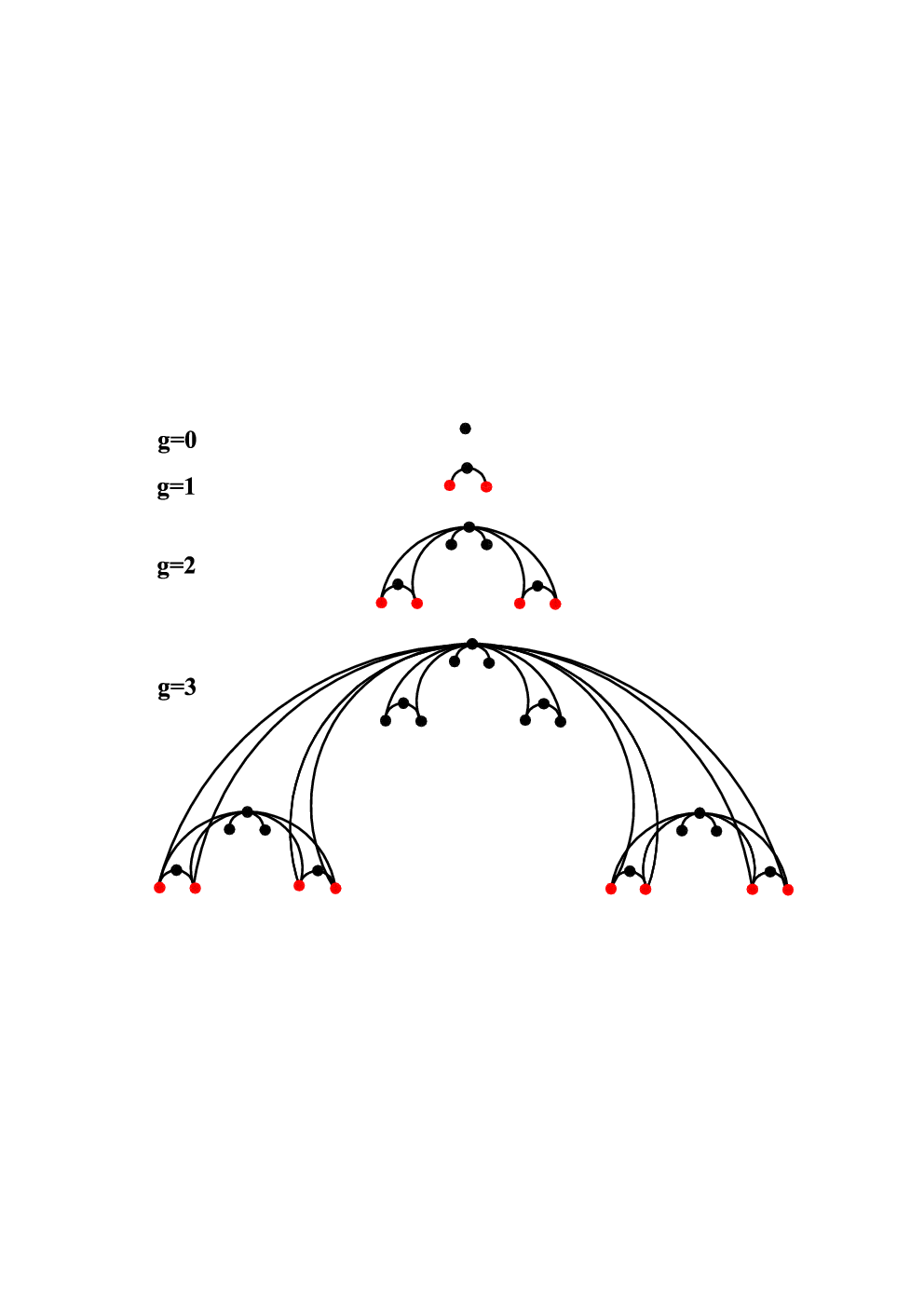
Some properties of the BRV model have been investigated in detail [37]. Let be the number of nodes in , the network of th generation. By construction, at each new iteration, the number of network nodes increases by a factor of three, which together with the initial condition leads to . In , the degree of all nodes and the number of nodes having the same degree can be determined exactly [37]. For example, the degree of the hub node is , and the degree of bottom nodes is . Again for instance, the cardinality, defined as the number of nodes in a set, of the set for the bottom nodes is . The network is a sparse one with the mean degree averaged over all nodes being which is approximately equal to in the limit of infinite .
The BRV model presents some typical properties of real-life systems [24, 37]. It is scale-free with the degree distribution exponent . In particular, the network has a crucial feature characterized by an obvious hierarchical structure that has also been observed in many real networks, e.g., metabolic networks [22, 27]. All these characteristics are not shared by other previous models. The peculiar structural characteristics make the network unique within the category of scale-free networks. It is the precursor, probably the first model for hierarchical scale-free networks. However, in spite of its importance, the rigorous knowledge of the average distance is still missing; its exact determination is the primary topic of this paper.
3 Closed-form solution to average distance
After introducing the hierarchical scale-free network, we now derive analytically the average distance. We represent all the shortest path lengths of network as a matrix in which the entry is the distance between nodes and that is the length of a shortest path joining and . A measure of the typical separation between two nodes in is given by the average distance defined as the mean of distances over all pairs of nodes:
| (1) |
where
| (2) |
denotes the sum of the distances between two nodes over all couples. Notice that in Eq. (2), for a pair of nodes and (), we only count or , not both.

We continue by exhibiting the procedure of determining the total distance and present the recurrence formula, which allows us to obtain of the generation from of the generation. The hierarchical network has a self-similar structure that allows one to calculate analytically. According to the construction, see figure 2, network is obtained by joining three copies of that are labeled as , , and . Using this self-similar property, the total distance satisfies the recursion relation
| (3) |
where is the sum over all shortest path length whose endpoints are not in the same branch. The paths that contribute to must all go through the hub node , where the three copies of are connected. Hence, to determine , all that is left is to calculate . The analytic expression for , referred to as the crossing path length, can be derived as below.
Let be the sum of the lengths of all shortest paths whose endpoints are in and , respectively. Then the total sum is given by
| (4) |
By symmetry, , so
| (5) |
Having in terms of the quantities of and , the next step is to explicitly determine the two quantities.
To calculate the crossing distance and , we give the following notation. For an arbitrary node in network , let be the smallest value of the shortest path length from to any of the bottom nodes belonging to , and the sum of for all nodes in is denoted by . Analogously, in let denote the distance from a node to the hub node , and let stand for the total distance between all nodes in and the hub node in , including itself. By definition, can be given by the sum
| (6) | |||||
and can be written recursively as
| (7) | |||||
Using , and considering and , the simultaneous equations (6) and (7) can be solved inductively to obtain:
| (8) |
and
| (9) |
With above obtained results, we can determine and , which can be expressed in terms of these explicitly determined quantities. By definition, is given by the sum
| (10) | |||||
Inserting Eqs. (8) and (9) into (10), we have
| (11) |
Proceeding similarly,
| (12) | |||||
Substituting Eqs. (11) and (12) into (5), we get
| (13) |
Substituting Eq. (13) into (3) and using the initial value , we can obtain the exact expression for the total distance
| (14) |
Then the analytic expression for average distance can be obtained as
| (15) |

We have checked our rigorous result provided by Eq. (15) against numerical calculations for different network order up to which corresponds to . In all the cases we obtain a complete agreement between our theoretical formula and the results of numerical investigation, see figure 3.
We continue to express the average distance as a function of network order , in order to obtain the scaling between these two quantities. Recalling that , we have . Hence Eq. (15) can be rewritten as
| (16) |
In the infinite network order limit, i.e.,
| (17) |
Thus, for large networks, the average distance grows logarithmically with increasing order of the network.
This logarithmic scaling is similar to that of other hierarchical scale-free networks with high clustering coefficient, which was previously obtained in a quite different way by mapping the system onto a Potts model in one-dimensional lattices [28]. Since there is no triangle in the studied network, its clustering coefficient is zero. Our result, together with earlier work, shows that clustering coefficient has no qualitative effect on the average distance of deterministic hierarchical scale-free networks, which is consistent with the phenomenon observed for random scale-free networks by using numerical simulations [39, 40].
However, the deterministic network under consideration also exhibits some different aspects from the conventional (non-hierarchical) scale-free networks. For example, it has been suggested that for stochastic scale-free networks with degree distribution exponent and network order , their average distance behaves as a double logarithmic scaling with : [7, 6], which is in sharp contrast to the logarithmic scaling obtained for the BRV model addressed here, in despite of the fact that the latter has a degree distribution exponent less than 3. Actually, this logarithmic scaling of average distance with network order has also been shown in other deterministic scale-free networks with [19, 25, 28, 36, 41, 42]. Thus, deterministic scale-free networks present an obvious difference from their stochastic scale-free counterparts in the aspect of structural property of average distance. We speculate that the logarithmic scaling for average distance can be used to establish the universality class for deterministic scale-free networks. Further studies are necessary to uncover the reasons for the similarity and dissimilarity between deterministic and random scale-free networks as regards average distance.
4 Conclusions
To conclude, scale-free behavior and hierarchical structure are ubiquitous in a variety of real-life systems. In this paper, we studied analytically the average distance of a deterministically growing scale-free hierarchical network introduced by Barabási, Ravasz and Vicsek [24], which can mimic some real-world networks to some extent. Based on the particular construction of the network, we obtained the rigorous solution to the average distance. We showed that in the infinite limit of network order , the average distance exhibits the scaling law as . We also showed that there are similarity and dissimilarity of the behaviors of average distance of deterministic and random scale-free networks. Finally, combining the obtained result and previous studies, we argued that the logarithmical scaling of average distance with network order may characterize deterministic scale-free networks.
Acknowledgment
This research was supported by the National Basic Research Program of China under grant No. 2007CB310806, the National Natural Science Foundation of China under Grant Nos. 60704044, 60873040 and 60873070, Shanghai Leading Academic Discipline Project No. B114, and the Program for New Century Excellent Talents in University of China (NCET-06-0376).
References
References
- [1] R. Albert and A.-L. Barabási, Rev. Mod. Phys. 74, 47 (2002).
- [2] S. N. Dorogovtsev and J. F. F. Mendes, Adv. Phys. 51, 1079 (2002).
- [3] M. E. J. Newman, SIAM Rev. 45, 167 (2003).
- [4] S. Boccaletti, V. Latora, Y. Moreno, M. Chavez and D.-U. Hwanga, Phys. Rep. 424, 175 (2006).
- [5] D. J. Watts and H. Strogatz, Nature (London) 393, 440 (1998).
- [6] F. Chung and L. Lu, Proc. Natl. Acad. Sci. U.S.A. 99, 15879 (2002).
- [7] R. Cohen and S. Havlin, Phys. Rev. Lett. 90, 058701 (2003).
- [8] S. N. Dorogovtsev, J. F. F. Mendes, and J. G. Oliveira, Phys. Rev. E 73, 056122 (2006).
- [9] C. Song, S. Havlin, H. A. Makse, Nature Phys. 2, 275 (2006).
- [10] Z. Z. Zhang, S. G. Zhou, and T. Zou, Eur. Phys. J. B 56, 259 (2007).
- [11] Z. Z. Zhang, S. G. Zhou, L. C. Chen, and J. H. Guan, Eur. Phys. J. B 64, 277 (2008).
- [12] S. Condamin, O. Bénichou, V. Tejedor, R. Voituriez, and J. Klafter, Nature (London) 450, 77 (2007).
- [13] T. Nishikawa, A. E. Motter, Y.-C. Lai, and F. C. Hoppensteadt, Phys. Rev. Lett. 91, 014101 (2003).
- [14] S. N. Dorogovtsev, J. F. F. Mendes, and A.N. Samukhin, Nucl. Phys. 653, 307 (2003).
- [15] W. S. Lovejoy, C. H. Loch, Soc. Netw. 25, 333 (2003).
- [16] A. Fronczak, P. Fronczak, and J. A. Hołyst, Phys. Rev. E 70, 056110 (2004).
- [17] J. A. Hołyst, J. Sienkiewicz, A. Fronczak, P. Fronczak, and K. Suchecki, Phys. Rev. E 72, 026108 (2005).
- [18] Z. Z. Zhang, S. G. Zhou, L. C. Chen, M. Yin, and J. H. Guan, J. Phys. A: Math. Theor. 41, 485102 (2008).
- [19] Z. Z. Zhang, L. C. Chen, L. J. Fang, S. G. Zhou, Y. C. Zhang, and J. H. Guan, J. Stat. Mech.: Theory Exp. (2009) P02034.
- [20] A. Fekete, G. Vattay, and M. Pósfai, Phys. Rev. E 79, 065101(R) (2009).
- [21] A.-L. Barabási and R. Albert, Science 286, 509 (1999).
- [22] E. Ravasz, A. L. Somera, D. A. Mongru. Z. N. Oltvai, and A.-L. Barabási, Science 297, 1551 (2002).
- [23] A. Clauset, C Moore, and M. E. J. Newman, Nature (London) 451, 98 (2008).
- [24] A.-L. Barabási, E. Ravasz, and T. Vicsek, Physica A 299, 559 (2001).
- [25] S. N. Dorogovtsev, A. V. Goltsev, and J. F. F. Mendes, Phys. Rev. E 65, 066122 (2002).
- [26] S. Jung, S. Kim, and B. Kahng, Phys. Rev. E 65, 056101 (2002).
- [27] E. Ravasz and A.-L. Barabási, Phys. Rev. E 67, 026112 (2003).
- [28] J. D. Noh, Phys. Rev. E 67, 045103(R) (2003).
- [29] J. D. Noh and H. Rieger, Phys. Rev. E 69, 036111 (2004).
- [30] M. Hinczewski and A. N. Berker, Phys. Rev. E 73, 066126 (2006).
- [31] H. D. Rozenfeld, S. Havlin, and D. ben-Avraham, New J. Phys. 9, 175 (2007).
- [32] M. Hinczewski, Phys. Rev. E 75, 061104 (2007).
- [33] Z. Z. Zhang, S. G. Zhou, T. Zou, L. C. Chen, and J. H. Guan, Eur. Phys. J. B 60, 259 (2007).
- [34] Z. Z. Zhang, S. G. Zhou, L. J. Fang, J. H. Guan, and Y. C. Zhang, EPL 79, 38007 (2007).
- [35] F. Comellas and A. Miralles, Physica A. 388, 2227 (2009).
- [36] Z. Z. Zhang, J. H. Guan, B. L. Ding, L. C. Chen, and S. G. Zhou, New J. Phys. 11, 083007 (2009).
- [37] K. Iguchi and H. Yamada, Phys. Rev. E 71, 036144 (2005).
- [38] E. Agliari and R. Burioni, Phys. Rev. E 80, 031125 (2009).
- [39] P. Holme and B. J. Kim, Phys. Rev. E 65, 026107 (2002).
- [40] Z. Z. Zhang, L. L. Rong, B. Wang, S. G. Zhou, and J. H. Guan, Physica A 380, 639 (2007).
- [41] Z. Z. Zhang, S. G. Zhou, and L. C. Chen, Eur. Phys. J. B 58, 337 (2007).
- [42] Z. Z. Zhang, L. C. Chen, S. G. Zhou, L. J. Fang, J. H. Guan, and T. Zou, Phys. Rev. E 77, 017102 (2008).