跳到论文正文
W Papers独立论文阅读器 arXiv:0910.5286 论文正文 计算阅读时间 · 0%
引用这篇论文根据当前论文元数据生成,正式投稿前建议核对。


License: arXiv.org perpetual non-exclusive license
arXiv:0910.5286v1 [math.NA] 28 Oct 2009

Discrete Fourier analysis with lattices on planar domainsThanks: The first authors was supported by NSFC Grants 10601056 and 10971212. The second author was supported by NSFC Grant 60970089 and National Basic Research Program Grant 2005CB321702.

Huiyuan Li Address: Institute of Software
Chinese Academy of Sciences
Beijing 100190, China
Email address: hynli@mail.rdcps.ac.cn
, Jiachang Sun Address: Institute of Software
Chinese Academy of Sciences
Beijing 100190, China
Email address: sun@mail.rdcps.ac.cn
and Yuan Xu Address:  Department of Mathematics
University of Oregon
Eugene, Oregon 97403-1222.
Email address: yuan@math.uoregon.edu
Date: August 24, 2026
Abstract.

A discrete Fourier analysis associated with translation lattices is developed recently by the authors. It permits two lattices, one determining the integral domain and the other determining the family of exponential functions. Possible choices of lattices are discussed in the case of lattices that tile ℝ2{\mathbb{R}}^{2} and several new results on cubature and interpolation by trigonometric, as well as algebraic, polynomials are obtained.

Key words and phrases: 
Discrete Fourier series, trigonometric, lattices, cubature, interpolation
1991 Mathematics Subject Classification
41A05, 41A10

1. Introduction

A framework of discrete Fourier analysis associated with translation tiling was developed recently in [7], based on the principle that if Ω\Omega is a bounded open set that tiles ℝd{\mathbb{R}}^{d} with the lattice L=A​ℤdL=A{\mathbb{Z}}^{d}, then the family of exponentials {e2​π​i​α⋅x:α∈L⟂}\{\mathrm{e}^{2\pi i\alpha\cdot x}:\alpha\in L^{\perp}\}, where L⟂=A−𝗍𝗋​ℤdL^{\perp}=A^{-{\mathsf{tr}}}{\mathbb{Z}}^{d} is the dual lattice of LL, forms an orthonormal basis in L2​(Ω)L^{2}(\Omega) ([4]). Our set up permits two lattices, one determining the integral domain and the other determining the exponentials that are orthogonal under the discrete inner product. The case that both lattices have the regular hexagon as fundamental domain was studied in [7] to illustrate the main set up, which leads to new cubature formula and Lagrange interpolation for trigonometric polynomials on hexagonal domains and equilateral triangles, as well as results for algebraic polynomials on the region bounded by Steiner’s hypocycloid. This is extended to three dimension in [9], giving results on cubature and interpolation on the rhombic dodecahedron and the tetrahedron, and further extended to ℝd{\mathbb{R}}^{d} in [10] for 𝒜d{\mathcal{A}}_{d} type lattice. In [8], the two lattices are chosen differently with fundamental domains being a square and a rhombic (rotation of the square by 90∘90^{\circ}), respectively. The choice leads to, surprisingly, one family of minimal cubature for product Chebyshev weight on [−1,1]2[-1,1]^{2}, first discovered by working with common zeros of orthogonal polynomials of two variables. An extension to three dimension gives a family of cubature formulas on the cube that have the smallest number of nodes among all known formulas, which coincides, rather surprisingly, with the cubature discovered in [11] by a totally different method.

The two lattices in [8] were chosen for the purpose of obtaining algebraic cubature formulas on the square. Its success prompts us to ask what other choices are possible. In the present paper, we try to answer this question in the case of ℝ2{\mathbb{R}}^{2}. Up to affine transforms, there are essentially two types of translation tiling in ℝ2{\mathbb{R}}^{2} with fundamental domain being either squares or regular hexagons. Their combinations in our discrete Fourier analysis, however, yield several distinct cases, including several cases not covered in our previous studies. One that is of particular interesting has one tiling sets as the regular hexagon and the other as the rotation of the regular hexagon by 90∘90^{\circ} (see Section 3.5), which leads to another set of cubature and interpolation on the equilateral triangle, different from those obtained in [7]. In order to present the main idea without being overwhelmed by notations and numerous formulas, we shall work mostly with cubature formulas, a central part but by no means all of discrete Fourier analysis, unless other results are deemed novel enough to warrant inclusion.

The paper is organized as follows. In the following section we recall the framework developed in [7] and use it to treat the classical product discrete Fourier analysis on the plane, which illustrates well what can be expected in the non-classical settings. Section 3 is divided into a number of subsections, each deals with one distinct choice of two lattices.

2. Discrete Fourier analysis with lattice

In the first subsection, we give a succinct recount of the framework of discrete Fourier analysis with tiling in [7]. We refer to [1] for lattices, tiling and various related topics, and refer to [2, 14] for some applications of discrete Fourier analysis in several variables. In the second subsection, we illustrate the general theory by using it to recover the classical product discrete Fourier analysis on the square.

2.1. Discrete Fourier analysis

A lattice LL in ℝd{\mathbb{R}}^{d} is a discrete subgroup L=LA:=A​ℤdL=L_{A}:=A{\mathbb{Z}}^{d}, where AA, called a generator matrix, is nonsingular. A bounded set Ω\Omega of ℝd{\mathbb{R}}^{d}, called the fundamental domain of LL, is said to tile ℝd{\mathbb{R}}^{d} with the lattice LL if

∑α∈LχΩ​(x+α)=1,for almost all x∈ℝd,\sum_{\alpha\in L}\chi_{\Omega}(x+\alpha)=1,\qquad\hbox{for almost all $x\in{\mathbb{R}}^{d}$},

where χΩ\chi_{\Omega} denotes the characteristic function of Ω\Omega. We write this as Ω+L=ℝd\Omega+L={\mathbb{R}}^{d}. For a given lattice LAL_{A}, the dual lattice LA⟂L_{A}^{\perp} is given by LA⟂=A−𝗍𝗋​ℤdL_{A}^{\perp}=A^{-{\mathsf{tr}}}{\mathbb{Z}}^{d}. According to a result of Fuglede [4], a bounded open set Ω\Omega tiles ℝd{\mathbb{R}}^{d} with the lattice LL if, and only, {e2​π​i​α⋅x:α∈L⟂}\{\mathrm{e}^{2\pi i\alpha\cdot x}:\alpha\in L^{\perp}\} is an orthonormal basis with respect to the inner product

(2.1) ⟨f,g⟩Ω=1mes⁡(Ω)​∫Ωf⁡(x)​g⁡(x)¯​𝑑x.\langle f,g\rangle_{\Omega}=\frac{1}{\mathrm{mes}(\Omega)}\int_{\Omega}f(x)\overline{g(x)}dx.

For L=A​ℤdL=A{\mathbb{Z}}^{d}, the measure of Ω\Omega is equal to |det(A)||\det(A)|. Since LA⟂=A−𝗍𝗋​ℤdL^{\perp}_{A}=A^{-{\mathsf{tr}}}{\mathbb{Z}}^{d}, we can write α=A−𝗍𝗋​k\alpha=A^{-{\mathsf{tr}}}k for α∈LA⟂\alpha\in L_{A}^{\perp} and k∈ℤdk\in{\mathbb{Z}}^{d}, so that e2​π​i​α⋅x=e2​π​i​k𝗍𝗋​A−1​x\mathrm{e}^{2\pi i\alpha\cdot x}=\mathrm{e}^{2\pi ik^{{\mathsf{tr}}}A^{-1}x}.

For our discrete Fourier analysis, the boundary of Ω\Omega matters. We shall fix an Ω\Omega such that 0∈Ω0\in\Omega and Ω+A​ℤd=ℝd\Omega+A{\mathbb{Z}}^{d}={\mathbb{R}}^{d} holds pointwisely and without overlapping.

Definition 2.1.

Let ΩA\Omega_{A} and ΩB\Omega_{B} be the fundamental domains of A​ℤdA{\mathbb{Z}}^{d} and B​ℤdB{\mathbb{Z}}^{d}, respectively. Assume all entries of the matrix N:=B𝗍𝗋​AN:=B^{\mathsf{tr}}A are integers. Define

ΛN:={k∈ℤd:B−𝗍𝗋​k∈ΩA}andΛN†:={k∈ℤd:A−𝗍𝗋​k∈ΩB}.\Lambda_{N}:=\{k\in{\mathbb{Z}}^{d}:B^{-{\mathsf{tr}}}k\in\Omega_{A}\}\quad\hbox{and}\quad\Lambda_{N}^{\dagger}:=\{k\in{\mathbb{Z}}^{d}:A^{-{\mathsf{tr}}}k\in\Omega_{B}\}.

Furthermore, define the finite dimensional subspace of exponential functions

ℋN:=span⁡{e2​π​i​k𝗍𝗋​A−1​x,k∈ΛN†}.{\mathcal{H}}_{N}:=\operatorname{span}\left\{\mathrm{e}^{2\pi i\,k^{\mathsf{tr}}A^{-1}x},\,k\in\Lambda_{N}^{\dagger}\right\}.

The main result in the discrete Fourier analysis is the following theorem:

Theorem 2.2.

Let A,BA,B and NN be as in Definition 2.1. Define

⟨f,g⟩N=1|det(N)|​∑j∈ΛNf⁡(B−𝗍𝗋​j)​g⁡(B−𝗍𝗋​j)¯\langle f,g\rangle_{N}=\frac{1}{|\det(N)|}\sum_{j\in\Lambda_{N}}f(B^{-{\mathsf{tr}}}j)\overline{g(B^{-{\mathsf{tr}}}j)}

for f,gf,g in C⁡(ΩA)C(\Omega_{A}), the space of continuous functions on ΩA\Omega_{A}. Then

(2.2) ⟨f,g⟩ΩA=⟨f,g⟩N,f,g∈ℋN.\langle f,g\rangle_{\Omega_{A}}=\langle f,g\rangle_{N},\qquad f,g\in{\mathcal{H}}_{N}.

It follows readily that (2.2) gives a cubature formula exact for functions in ℋN{\mathcal{H}}_{N}. Furthermore, it also implies a Lagrange interpolation by exponential functions. Let ℐN​f{\mathcal{I}}_{N}f denote the Fourier expansion of ff in ℋN{\mathcal{H}}_{N} with respect to the inner product ⟨⋅,⋅⟩N\langle\cdot,\cdot\rangle_{N}, which can be expressed as

(2.3) ℐN​f​(x)=∑k∈ΛNf⁡(B−𝗍𝗋​k)​ΨΩBA​(x−B−𝗍𝗋​k),f∈C⁡(ΩA),{\mathcal{I}}_{N}f(x)=\sum_{k\in\Lambda_{N}}f(B^{-{\mathsf{tr}}}k)\Psi_{\Omega_{B}}^{A}(x-B^{-{\mathsf{tr}}}k),\qquad f\in C(\Omega_{A}),

where

(2.4) ΨΩBA​(x)=1|det(N)|​∑j∈ΛN†e2​π​i​j𝗍𝗋​A−1​x.\Psi_{\Omega_{B}}^{A}(x)=\frac{1}{|\det(N)|}\sum_{j\in\Lambda_{N}^{{\dagger}}}\mathrm{e}^{2\pi ij^{\mathsf{tr}}A^{-1}x}.
Theorem 2.3.

Let A,BA,B and NN be as in Definition 2.1. Then ℐN{\mathcal{I}}_{N} is the unique interpolation operator on NN in ℋN{\mathcal{H}}_{N}; that is,

ℐN​f​(B−𝗍𝗋​j)=f⁡(B−𝗍𝗋​j),∀j∈ΛN.{\mathcal{I}}_{N}f(B^{-{\mathsf{tr}}}j)=f(B^{-{\mathsf{tr}}}j),\qquad\forall j\in\Lambda_{N}.

In particular, #​ΛN=#​ΛN𝗍𝗋=|det(N)|\#\Lambda_{N}=\#\Lambda_{N^{\mathsf{tr}}}=|\det(N)|. The cubature formula and the Lagrange interpolation are for functions that are periodic with respect to the lattice A​ℤdA{\mathbb{Z}}^{d}, which are functions satisfying

f⁡(x+A​k)=f⁡(x)for all k∈ℤd.f(x+Ak)=f(x)\qquad\hbox{for all $k\in{\mathbb{Z}}^{d}$}.

The function x↦e2​π​i​k𝗍𝗋​A−1​xx\mapsto\mathrm{e}^{2\pi ik^{\mathsf{tr}}A^{-1}x} is periodic with respect to the lattice A​ℤdA{\mathbb{Z}}^{d}.

2.2. Classical discrete Fourier analysis

We deduce the classical result on the plane (cf. [2, 23]) from the general theory described above. As mentioned in the introduction, we shall limit our consideration to cubature formulas. The result hints at what is possible in the non-classical cases in the rest of the paper.

For n∈ℕn\in{\mathbb{N}}, let A=IA=I, the identity matrix, and B=2​n​IB=2nI. Then N=B𝗍𝗋​A=2​n​IN=B^{\mathsf{tr}}A=2nI has all integer entries. Let ΩA=[−12,12)2\Omega_{A}=[-\frac{1}{2},\frac{1}{2})^{2}, which tiles ℝ2{\mathbb{R}}^{2} with ℤ2{\mathbb{Z}}^{2} pointwisely and without overlapping. We shall write Λn\Lambda_{n}, Λn†\Lambda_{n}^{\dagger}, ℋn{\mathcal{H}}_{n} in place of ΛN\Lambda_{N}, ΛN†\Lambda_{N}^{\dagger}, ℋN{\mathcal{H}}_{N}. Then

Λn=Λn†={k∈ℤ2:k∈[−n,n)2}andℋn=span{e2​π​i​k⋅x:k∈Λn†}.\Lambda_{n}=\Lambda_{n}^{\dagger}=\{k\in{\mathbb{Z}}^{2}:k\in[-n,n)^{2}\}\quad\hbox{and}\quad{\mathcal{H}}_{n}=\operatorname{span}\{\mathrm{e}^{2\pi ik\cdot x}:k\in\Lambda_{n}^{\dagger}\}.

It is clear that #​Λn=(2​n)2\#\Lambda_{n}=(2n)^{2}. The equation (2.2) in this setting becomes

(2.5) ∫[−12,12]2f⁡(x)​g⁡(x)¯​𝑑x=14​n2​∑k1=−nn−1∑k2=−nn−1f⁡(k12​n,k22​n)​g⁡(k12​n,k22​n)¯,f,g∈ℋn.\int_{[-\frac{1}{2},\frac{1}{2}]^{2}}f(x)\overline{g(x)}dx=\frac{1}{4n^{2}}\sum_{k_{1}=-n}^{n-1}\sum_{k_{2}=-n}^{n-1}f(\tfrac{k_{1}}{2n},\tfrac{k_{2}}{2n})\overline{g(\tfrac{k_{1}}{2n},\tfrac{k_{2}}{2n})},\quad f,g\in{\mathcal{H}}_{n}.

To illustrate what can be done on cubature, we state the results in stages.

Stage 1. It is easy to see that (2.5) yields a cubature formula

(2.6) ∫[−12,12]2f⁡(x)​𝑑x=14​n2​∑k1=−nn−1∑k2=−nn−1f⁡(k12​n,k22​n),∀f∈ℋ2​n−1∗,\displaystyle\int_{[-\frac{1}{2},\frac{1}{2}]^{2}}f(x)dx=\frac{1}{4n^{2}}\sum_{k_{1}=-n}^{n-1}\sum_{k_{2}=-n}^{n-1}f(\tfrac{k_{1}}{2n},\tfrac{k_{2}}{2n}),\qquad\forall f\in{\mathcal{H}}_{2n-1}^{*},

where ℋn∗:=span⁡{e2​π​i​k⋅x:k∈[−n,n]2∩ℤ2}{\mathcal{H}}_{n}^{*}:=\operatorname{span}\{\mathrm{e}^{2\pi ik\cdot x}:k\in[-n,n]^{2}\cap{\mathbb{Z}}^{2}\}. The set of nodes of cubature (2.6) is not symmetric on [−12,12]2[-\frac{1}{2},\frac{1}{2}]^{2}, since it has points on only part of the boundary of the square. We would like to have cubature whose nodes is symmetric on the square.

Stage 2. We construct cubature formulas for ℋ2​n−1∗{\mathcal{H}}_{2n-1}^{*} that have symmetric nodes on the square. Such a cubature is invariant under sign changes in both variables. We can in fact obtain two such formulas from (2.6). The first one is obtained upon using the periodicity of the functions in the sums in the right hand side,

(2.7) ∫[−12,12]2f⁡(x)​𝑑x=14​n2​∑k1=−nn∑k2=−nnck,n​f​(k12​n,k22​n),∀f∈ℋ2​n−1∗,\displaystyle\int_{[-\frac{1}{2},\frac{1}{2}]^{2}}f(x)dx=\frac{1}{4n^{2}}\sum_{k_{1}=-n}^{n}\sum_{k_{2}=-n}^{n}c_{k,n}f(\tfrac{k_{1}}{2n},\tfrac{k_{2}}{2n}),\qquad\forall f\in{\mathcal{H}}_{2n-1}^{*},

where ck,n=1c_{k,n}=1 if k∈(−n,n)2k\in(-n,n)^{2}, ck,n=1/2c_{k,n}=1/2 if either k1=±nk_{1}=\pm n or k2=±nk_{2}=\pm n but not both, and ck,n=1/4c_{k,n}=1/4 if k=(±n,±n)k=(\pm n,\pm n). The second one is obtained by applying (2.6) to the function f(⋅+14​n)f(\cdot+\frac{1}{4n}) and using the periodicity of ff in the integral,

(2.8) ∫[−12,12]2f⁡(x)​𝑑x=14​n2​∑k1=−nn−1∑k2=−nn−1f⁡(k1+122​n,k2+122​n),f∈ℋ2​n−1∗.\displaystyle\int_{[-\frac{1}{2},\frac{1}{2}]^{2}}f(x)dx=\frac{1}{4n^{2}}\sum_{k_{1}=-n}^{n-1}\sum_{k_{2}=-n}^{n-1}f(\tfrac{k_{1}+\frac{1}{2}}{2n},\tfrac{k_{2}+\frac{1}{2}}{2n}),\qquad f\in{\mathcal{H}}_{2n-1}^{*}.

The fact that the set of nodes in either (2.7) or (2.8) is invariant under the group ℤ22{\mathbb{Z}}_{2}^{2} (sign changes) allows us to derive cubature formulas for product cosine and produce sine functions. Let 𝒯Cn:=span{cos2πk1x1cos2πk2x2:0≤k1,k2≤n}{\mathcal{T}\!C}_{n}:=\operatorname{span}\{\cos 2\pi k_{1}x_{1}\cos 2\pi k_{2}x_{2}:0\leq k_{1},k_{2}\leq n\} and 𝒯Sn:=span{sin2πk1x1sin2πk2x2:1≤k1,k2≤n}{\mathcal{T}\!S}_{n}:=\operatorname{span}\{\sin 2\pi k_{1}x_{1}\sin 2\pi k_{2}x_{2}:1\leq k_{1},k_{2}\leq n\}, which consist of functions in ℋn∗{\mathcal{H}}_{n}^{*} that are invariant or anti-invariant under ℤ22{\mathbb{Z}}_{2}^{2}, respectively.

Stage 3. Restricting (2.8) to 𝒯​C2​n−1{\mathcal{T}\!C}_{2n-1}, we obtain a trigonometric cubature,

(2.9) ∫[0,12]2f⁡(x)​𝑑x=14​n2​∑k1=0n−1∑k2=0n−1f⁡(k1+122​n,k2+122​n),∀f∈𝒯​C2​n−1,\int_{[0,\frac{1}{2}]^{2}}f(x)dx=\frac{1}{4n^{2}}\sum_{k_{1}=0}^{n-1}\sum_{k_{2}=0}^{n-1}f(\tfrac{k_{1}+\frac{1}{2}}{2n},\tfrac{k_{2}+\frac{1}{2}}{2n}),\qquad\forall f\in{\mathcal{T}\!C}_{2n-1},

whereas restricting (2.7) to 𝒯​C2​n−1{\mathcal{T}\!C}_{2n-1} gives another trigonometric cubature for 𝒯​C2​n−1{\mathcal{T}\!C}_{2n-1}. Furthermore, restricting (2.7) or (2.8) to 𝒯​S2​n−1{\mathcal{T}\!S}_{2n-1} leads to cubature for 𝒯​S2​n−1{\mathcal{T}\!S}_{2n-1}.

The Chebyshev polynomials of the first and the second kind are defined, respectively, by Tn​(ξ)=cos⁡2​π​n​θT_{n}(\xi)=\cos 2\pi n\theta and Un​(ξ)=sin⁡2​π​(n+1)​θ/sin⁡2​π​θU_{n}(\xi)=\sin 2\pi(n+1)\theta/\sin 2\pi\theta, where ξ=cos⁡2​π​θ\xi=\cos 2\pi\theta with 0≤θ≤1/20\leq\theta\leq 1/2. These are orthogonal polynomials with respect to w0(ξ):=(1−ξ2)−1/2w_{0}(\xi):=(1-\xi^{2})^{-1/2} and w1​(ξ):=(1−ξ2)1/2w_{1}(\xi):=(1-\xi^{2})^{1/2}, respectively, on [−1,1][-1,1]. Consequently, under the change of variables

(2.10) (x1,x2)↦(y1,y2)=(cos⁡2​π​x1,cos⁡2​π​x2)∈[−1,1]2,(x_{1},x_{2})\mapsto(y_{1},y_{2})=(\cos 2\pi x_{1},\cos 2\pi x_{2})\in[-1,1]^{2},

the space 𝒯​Cn{\mathcal{T}\!C}_{n} is mapped into the product space Πn×Πn\Pi_{n}\times\Pi_{n}, where Πn\Pi_{n} denotes the space of algebraic polynomials of one variable, and 𝒯​Sn{\mathcal{T}\!S}_{n} is mapped into Πn−1×Πn−1\Pi_{n-1}\times\Pi_{n-1}.

Stage 4. Under the map x↦yx\mapsto y of (2.10), the cubature (2.9) becomes

(2.11) 1π2​∫[−1,1]2f⁡(y)​W0​(y)​𝑑y=1n2​∑k1=0n−1∑k2=0n−1f⁡(cos⁡π⁡(2​k1+1)2​n,cos⁡π⁡(2​k2+1)2​n),\frac{1}{\pi^{2}}\int_{[-1,1]^{2}}f(y)W_{0}(y)dy=\frac{1}{n^{2}}\sum_{k_{1}=0}^{n-1}\sum_{k_{2}=0}^{n-1}f(\cos\tfrac{\pi(2k_{1}+1)}{2n},\cos\tfrac{\pi(2k_{2}+1)}{2n}),

for f∈Π2​n−1×Π2​n−1f\in\Pi_{2n-1}\times\Pi_{2n-1}, where W0​(y)=w0​(y1)​w0​(y2)W_{0}(y)=w_{0}(y_{1})w_{0}(y_{2}), which is in fact the product Chebyshev-Gauss cubature of the first kind. Applying the same procedure on the cubature (2.7), we obtain the product Chebyshev-Gauss-Lobatto cubature. Furthermore, if we apply this procedure on the cubature for 𝒯​S2​n−1{\mathcal{T}\!S}_{2n-1} that were mentioned in Stage 3, we obtain the product cubature for the product Chebyshev weight W1​(y)=w1​(y1)​w1​(y2)W_{1}(y)=w_{1}(y_{1})w_{1}(y_{2}) of the second kind.

3. Discrete Fourier analysis on planer domains

We now apply the general theory in Section 2.1 on the non-classical choices of lattices. The guideline of our choices is the program that we outlined for the classical case in subsection 2.2. We list the cases according to the shapes of the fundamental domains of lattices. For example, the classical case in Section 2.2 is Square-Square. The main ones that we consider are the regular domains such as square, rhombus, and regular hexagon, which are depicted below.

Refer to caption
Refer to caption
Figure 1. Square, rhombus, regular hexagon

3.1. Square-Rhombus

In this case we choose A=IA=I with ΩA=[−12,12)2\Omega_{A}=[-\frac{1}{2},\frac{1}{2})^{2} being the square and choose B=n​RB=nR, where R​ℤ2R{\mathbb{Z}}^{2} has rhombic as its fundamental domain,

R:=[11−11]withΩB={x∈ℝ2:−n≤x1+x2<n,−n≤x2−x1<n}.R:=\left[\begin{matrix}1&1\\ -1&1\end{matrix}\right]\quad\hbox{with}\quad\Omega_{B}=\{x\in{\mathbb{R}}^{2}:-n\leq x_{1}+x_{2}<n,\,\,-n\leq x_{2}-x_{1}<n\}.

This case was studied in [8]. We shall be brief. Here ΛN=ΛN†=:Λn\Lambda_{N}=\Lambda_{N}^{\dagger}=:\Lambda_{n}, where

Λn={j∈ℤ2:−n≤j2±j1<n}andΛn∗:={j∈ℤ2:−n≤j2±j1≤n}.\Lambda_{n}=\{j\in{\mathbb{Z}}^{2}:-n\leq j_{2}\pm j_{1}<n\}\quad\hbox{and}\quad\Lambda_{n}^{*}:=\{j\in{\mathbb{Z}}^{2}:-n\leq j_{2}\pm j_{1}\leq n\}.

The set Λn\Lambda_{n} is not symmetric on [−n,n]2[-n,n]^{2} but Λn∗\Lambda_{n}^{*} is. The cardinality of Λn\Lambda_{n} is |Λn|=2​n2|\Lambda_{n}|=2n^{2}. We follow the program in Section 2.2: In Stage 1 we deduce a cubature from Theorem 2.2, which has nodes indexed by Λn\Lambda_{n}, then in Stage 2 we derive a cubature by periodicity that has nodes indexed by Λn∗\Lambda_{n}^{*}. By considering functions that are even in both variables, we deduce in Stage 3 a cubature for trigonometric polynomials, which we state as follows. Changing variables from jj to k=2​n​B−𝗍𝗋​jk=2nB^{-{\mathsf{tr}}}j, or k1=j1+j2k_{1}=j_{1}+j_{2} and k2=j2−j1k_{2}=j_{2}-j_{1}, it follows easily that j∈Λn∗j\in\Lambda_{n}^{*} is equivalent to

k∈Xn∗={2k:−n2≤k1,k2≤n2}∪{2k+1:−n+12≤k1,k2≤n−12}.k\in X_{n}^{*}=\left\{2k:-\tfrac{n}{2}\leq k_{1},k_{2}\leq\tfrac{n}{2}\}\cup\{2k+1:-\tfrac{n+1}{2}\leq k_{1},k_{2}\leq\tfrac{n-1}{2}\right\}\!.

Let Xn∘X_{n}^{\circ}, XneX_{n}^{e} and XnvX_{n}^{v} denote the set of points in Xn∗X_{n}^{*} that lie in the interior, the edges excluding corners, and the corners of [−n,n]2[-n,n]^{2}, respectively.

Throughout the rest of the paper, we will adopt the convention that X∘X^{\circ}, XeX^{e} and XvX^{v} are subsets of XX defined as above, whenever the domain to which the interior, edges and corners relate to is clear.

Theorem 3.1.

For n≥2n\geq 2, the cubature formula

(3.1) ∫[−12,12]2f⁡(x)​𝑑x=12​n2​∑k∈Xn∗ck(n)​f​(k2​n)withck(n)={1,k∈Xn∘12,k∈Xne14,k∈Xnv\int_{[-\frac{1}{2},\frac{1}{2}]^{2}}f(x)dx=\frac{1}{2n^{2}}\sum_{k\in X_{n}^{*}}c_{k}^{(n)}f(\tfrac{k}{2n})\quad\hbox{with}\quad c_{k}^{(n)}=\begin{cases}1,&k\in X_{n}^{\circ}\\ \frac{1}{2},&k\in X_{n}^{e}\\ \frac{1}{4},&k\in X_{n}^{v}\end{cases}

is exact for f∈𝒯2​n−1∗f\in{\mathcal{T}}_{2n-1}^{*}, where 𝒯m∗:=span⁡{e2​π​i​k⋅x:k∈Λm∗}.{\mathcal{T}}_{m}^{*}:=\mathrm{span}\left\{\mathrm{e}^{2\pi i\,k\cdot x}:\ k\in\Lambda_{m}^{*}\right\}.

The index set Λn∗\Lambda_{n}^{*} is most suitable for dealing with algebraic polynomials. In fact, under the change of variables x↦yx\mapsto y in (2.10), the space 𝒯​Cm∗{\mathcal{T}\!C}_{m}^{*} becomes the space Πm2\Pi_{m}^{2} of algebraic polynomial of total degree mm and the cubature (3.1) becomes a cubature for the product Chebyshev weight W0​(y)W_{0}(y) that is exact for Π2​n−12\Pi_{2n-1}^{2}. Let

Ξn:={(2k1,2k2):0≤k1,k2≤n2}∪{(2k1+1,2k2+1):0≤k1,k2≤n−12}.\Xi_{n}:=\{(2k_{1},{2k_{2}}):0\leq k_{1},k_{2}\leq\tfrac{n}{2}\}\cup\{({2k_{1}+1},{2k_{2}+1}):0\leq k_{1},k_{2}\leq\tfrac{n-1}{2}\}.

Then, in Stage 4, (3.1) becomes the following:

Theorem 3.2.

Let zk=(cos⁡k1​πn,cos⁡k2​πn)z_{k}=(\cos\frac{k_{1}\pi}{n},\cos\frac{k_{2}\pi}{n}). Then the cubature below is exact for f∈Π2​n−12f\in\Pi_{2n-1}^{2},

(3.2) 1π2​∫[−1,1]2f⁡(y)​W0​(y)​𝑑y=12​n2​∑k∈Ξnλk(n)​f​(zk),λk(n):={4,k∈Ξn∘,2,k∈Ξne,1,k∈Ξnv.\frac{1}{\pi^{2}}\int_{[-1,1]^{2}}f(y)W_{0}(y)dy=\frac{1}{2n^{2}}\sum_{k\in\Xi_{n}}\lambda_{k}^{(n)}f(z_{k}),\quad\lambda_{k}^{(n)}:=\begin{cases}4,&k\in\Xi_{n}^{\circ},\\ 2,&k\in\Xi_{n}^{e},\\ 1,&k\in\Xi_{n}^{v}.\end{cases}

The cardinality of Ξn\Xi_{n} is |Ξn|=n⁡(n+1)2+⌊n2⌋+1|\Xi_{n}|=\frac{n(n+1)}{2}+\lfloor\frac{n}{2}\rfloor+1, which is just one more than the theoretic lower bound for all such cubature ([3, 12]). The formula (3.2) first appeared in [20], where it is constructed by considering the common zeros of orthogonal polynomials of two variables; see also [13]. We can also derive similarly cubature for the product Chebyshev weight W1​(y)W_{1}(y) of the second kind.

The Lagrange interpolation polynomials based on the points in Ξn\Xi_{n} were defined and studied in [21]. The result there has also been recovered in [8], with (2.3) as the starting point, by utilizing the discrete Fourier analysis.

3.2. Rhombic-Square

In this case we choose A=RA=R with fundamental domain ΩR={x∈ℝ2:−1≤x2±x1<1}\Omega_{R}=\{x\in{\mathbb{R}}^{2}:-1\leq x_{2}\pm x_{1}<1\}, the rhombic, and B=n​IB=nI. Again write Λn\Lambda_{n} … in place of ΛN\Lambda_{N} …. It is then easy to verify that Λn=Λn†\Lambda_{n}=\Lambda_{n}^{\dagger} with

Λn={j∈ℤ2:−n≤k2±k1<n}andΛn∗:={j∈ℤ2:−n≤k2±k1≤n}.\Lambda_{n}=\{j\in{\mathbb{Z}}^{2}:-n\leq k_{2}\pm k_{1}<n\}\quad\hbox{and}\quad\Lambda_{n}^{*}:=\{j\in{\mathbb{Z}}^{2}:-n\leq k_{2}\pm k_{1}\leq n\}.

Furthermore, the space of exponential functions ℋn{\mathcal{H}}_{n} is given by

ℋn={eπ​i​((k1+k2)​x1+(k2−k1)​x2):k∈Λn}{\mathcal{H}}_{n}=\{\mathrm{e}^{\pi i((k_{1}+k_{2})x_{1}+(k_{2}-k_{1})x_{2})}:k\in\Lambda_{n}\}

and ℋn∗{\mathcal{H}}_{n}^{*} is likewise defined in terms of Λn∗\Lambda_{n}^{*}. Changing variables shows that

ℋn∗:={eπ​i​(j1​x1+j2​x2):−n≤j1,j2≤n,j1≡j2(mod2)}.{\mathcal{H}}_{n}^{*}:=\{\mathrm{e}^{\pi i(j_{1}x_{1}+j_{2}x_{2})}:-n\leq j_{1},j_{2}\leq n,\,\,j_{1}\equiv j_{2}\pmod{2}\}.

Following the program in Section 2.1, it is easy to see that the cubature in Stage 2 that has symmetric set of nodes, indexed by Λn∗\Lambda_{n}^{*}, takes the form

(3.3) 12​∫ΩRf⁡(x)​𝑑x=12​n2​∑k∈Λn∗ck,n​f​(kn),f∈ℋ2​n−1∗,ck,n={1,k∈Λn∘,12,k∈Λne,14,k∈Λnv.\frac{1}{2}\int_{\Omega_{R}}f(x)dx=\frac{1}{2n^{2}}\sum_{k\in\Lambda_{n}^{*}}c_{k,n}f(\tfrac{k}{n}),\quad f\in{\mathcal{H}}_{2n-1}^{*},\quad c_{k,n}=\begin{cases}1,&k\in\Lambda_{n}^{\circ},\\ \frac{1}{2},&k\in\Lambda_{n}^{e},\\ \frac{1}{4},&k\in\Lambda_{n}^{v}.\end{cases}

The subspace of functions in ℋn∗{\mathcal{H}}_{n}^{*} that are even in both variables becomes

(3.4) 𝒯n:=span{cosπj1x1cosπj2x2:0≤j1,j2≤n,j1≡j2(mod2)}.{\mathcal{T}}_{n}:=\operatorname{span}\{\cos\pi j_{1}x_{1}\cos\pi j_{2}x_{2}:0\leq j_{1},j_{2}\leq n,\,\,j_{1}\equiv j_{2}\pmod{2}\}.

For functions in 𝒯2​n−1{\mathcal{T}}_{2n-1}, we only need to consider the triangle TR:={x:0≤x1,x2,x1+x2≤1}T_{R}:=\{x:0\leq x_{1},x_{2},\,\ x_{1}+x_{2}\leq 1\}. Thus, in Stage 3, cubature (3.3) becomes

(3.5) 2​∫TRf⁡(x)​𝑑x=12​n2​∑k∈Ξnλk,n​f​(kn),f∈𝒯2​n−1,2\int_{T_{R}}f(x)dx=\frac{1}{2n^{2}}\sum_{k\in\Xi_{n}}\lambda_{k,n}f(\tfrac{k}{n}),\qquad f\in{\mathcal{T}}_{2n-1},

where TRT_{R} is the triangular domain Ξn={(k1,k2):0≤k1,k2,k1+k2≤n}\Xi_{n}=\{(k_{1},k_{2}):0\leq k_{1},k_{2},k_{1}+k_{2}\leq n\}, and λk,n=4\lambda_{k,n}=4 if k∈Ξn∘k\in\Xi_{n}^{\circ}, λk,n=2\lambda_{k,n}=2 if k∈Ξnek\in\Xi_{n}^{e}, λ(0,0),n=1\lambda_{(0,0),n}=1, and λ(n,0),n=λ(0,n),n=1/2\lambda_{(n,0),n}=\lambda_{(0,n),n}=1/2.

Under the mapping x↦y=(cos⁡π​x1,cos⁡π​x2)x\mapsto y=(\cos\pi x_{1},\cos\pi x_{2}), the boundary x1+x2=1x_{1}+x_{2}=1 of the triangle TRT_{R} is mapped onto y1+y2=0y_{1}+y_{2}=0, so that TRT_{R} is mapped onto the triangle TS={(y,y2):−1≤y1,y2≤1,y1+y2≥0}T_{S}=\{(y_{,}y_{2}):-1\leq y_{1},y_{2}\leq 1,y_{1}+y_{2}\geq 0\}, which is half of the square [−1,1]2[-1,1]^{2}. The cubature (3.5) in Stage 4 becomes a cubature with respect to the product Chebyshev weight W0W_{0} over TST_{S} that is exact for the subspace of polynomials Π2​n−1∗={Tk1(x1)Tk2(x2):0≤k1,k2≤2n−1,k1≡k2(mod2)}\Pi_{2n-1}^{*}=\{T_{k_{1}}(x_{1})T_{k_{2}}(x_{2}):0\leq k_{1},k_{2}\leq 2n-1,k_{1}\equiv k_{2}\pmod{2}\}, the image of 𝒯2​n−1{\mathcal{T}}_{2n-1} under the same mapping. Since Πn∗\Pi_{n}^{*} does not contain polynomials of total degree, we shall not write this cubature explicitly out. It is easy to see, however, that this cubature is in fact half of the product Chebyshev-Gaussian-Lobatto cubature, in the sense that its domain is half and it is exact for half of the polynomials of the latter cubature.

3.3. Rhombic-Rhombic

Here we choose A=RA=R and B=n​R−𝗍𝗋=n2​AB=nR^{-{\mathsf{tr}}}=\frac{n}{2}A, so that N=B𝗍𝗋​A=n​IN=B^{{\mathsf{tr}}}A=nI have integer entries. Then ΩA=ΩR\Omega_{A}=\Omega_{R} as in the previous case. Again denote ΛN\Lambda_{N}, … by Λn\Lambda_{n}, … . It is easy to see that Λn=Λn†\Lambda_{n}=\Lambda_{n}^{\dagger} with

Λn={j∈ℤ2:−n2≤−j1,j2<n2}andΛn∗:={j∈ℤ2:−n2≤j1,j2≤n2}.\Lambda_{n}=\{j\in{\mathbb{Z}}^{2}:-\tfrac{n}{2}\leq-j_{1},j_{2}<\tfrac{n}{2}\}\quad\hbox{and}\quad\Lambda_{n}^{*}:=\{j\in{\mathbb{Z}}^{2}:-\tfrac{n}{2}\leq j_{1},j_{2}\leq\tfrac{n}{2}\}.

Moreover, the space of exponential functions ℋn{\mathcal{H}}_{n} is given by, as in Section 3.2,

ℋn={eπ​i​((k1+k2)​x1+(k2−k1)​x2):k∈Λn}{\mathcal{H}}_{n}=\{\mathrm{e}^{\pi i((k_{1}+k_{2})x_{1}+(k_{2}-k_{1})x_{2})}:k\in\Lambda_{n}\}

and ℋn∗{\mathcal{H}}_{n}^{*} is likewise defined with Λn\Lambda_{n} replaced by Λn∗\Lambda_{n}^{*}. In this case, the cubature derived from Theorem 2.2, in Stage 1, takes the form

(3.6) 12​∫ΩRf⁡(x)​𝑑x=1n2​∑k∈Λnf⁡(k1+k2n,k2−k1n),∀f∈ℋ2​n−1∗.\frac{1}{2}\int_{\Omega_{R}}f(x)dx=\frac{1}{n^{2}}\sum_{k\in\Lambda_{n}}f(\tfrac{k_{1}+k_{2}}{n},\tfrac{k_{2}-k_{1}}{n}),\quad\forall f\in{\mathcal{H}}_{2n-1}^{*}.

The set of nodes of this cubature is on ΩR\Omega_{R}, and it contains no points on the boundary of ΩR\Omega_{R} when nn is an odd integer, whereas it contains points on half of the boundary of ΩR\Omega_{R} when nn is an even integer. In the latter case, we can again derive a cubature, exact for ℋ2​n−1∗{\mathcal{H}}_{2n-1}^{*}, that has notes indexed by Λn∗\Lambda_{n}^{*} as in Stage 2. Let us consider, however, only the case of nn being an odd integer below. As can be seen upon changing variables j1=k1+k2j_{1}=k_{1}+k_{2} and j2=k2−k1j_{2}=k_{2}-k_{1}, the subspace of functions in ℋn∗{\mathcal{H}}_{n}^{*} that are even in both variables is exactly 𝒯n{\mathcal{T}}_{n} in (3.4). Thus, just like in the case of Rhombic-Square, restricting (3.6) to functions in ℋ2​n−1∗{\mathcal{H}}_{2n-1}^{*} that are even in both variables, we deduce a cubature of Stage 3 on the triangle TRT_{R},

(3.7) 2​∫TRf⁡(x)​𝑑x=1n2​∑k∈Ξnλk,n​f​(k1+k2n,k2−k1n),∀f∈𝒯2​n−1,2\int_{T_{R}}f(x)dx=\frac{1}{n^{2}}\sum_{k\in\Xi_{n}}\lambda_{k,n}f(\tfrac{k_{1}+k_{2}}{n},\tfrac{k_{2}-k_{1}}{n}),\qquad\forall f\in{\mathcal{T}}_{2n-1},

where Ξn={(k1,k2):0≤k1,k2,k1+k2≤n2}\Xi_{n}=\{(k_{1},k_{2}):0\leq k_{1},k_{2},k_{1}+k_{2}\leq\frac{n}{2}\}; λk,n=4\lambda_{k,n}=4 if k∈Ξn∘k\in\Xi_{n}^{\circ}, λk,n=2\lambda_{k,n}=2 if either k1=0k_{1}=0 or k2=0k_{2}=0 or k1+k2=n2k_{1}+k_{2}=\frac{n}{2} but not both (i.e.,k∈Ξnek\in\Xi_{n}^{e}), and λ(0,0),n=1\lambda_{(0,0),n}=1, λ(0,n),n=1\lambda_{(0,n),n}=1 .

Finally, under the mapping x↦y=(cos⁡π​x1,cos⁡π​x2)x\mapsto y=(\cos\pi x_{1},\cos\pi x_{2}), the cubature (3.7) becomes a cubature with respect to the product Chebyshev weight W0W_{0} over the triangle domain TST_{S} for the polynomial subspace Π2​n−1∗\Pi_{2n-1}^{*} defined in the previous subsection. This cubature is exactly half of the algebraic cubature in the Square-Rhombic case.

3.4. Hexagon-Hexagon

In this case we choose A=HA=H and B=n2​HB=\frac{n}{2}H, where

H=(30−12)withΩH={x∈ℝ2:−1≤x2,3​x12±x22<1}.H=\begin{pmatrix}\sqrt{3}&0\\ -1&2\end{pmatrix}\quad\hbox{with}\quad\Omega_{H}=\left\{x\in{\mathbb{R}}^{2}:\ -1\leq x_{2},\tfrac{\sqrt{3}x_{1}}{2}\pm\tfrac{x_{2}}{2}<1\right\}.

This case was studied in [7]. We shall be brief, but recall necessary definitions that are needed in the following subsection. As shown in [7, 19], it is more convenient to use homogeneous coordinates (t1,t2,t3)(t_{1},t_{2},t_{3}) defined by

(3.8) (t1t2t3)=(32−1201−32−12)​(x1x2):=E​x,\displaystyle\begin{pmatrix}t_{1}\\ t_{2}\\ t_{3}\end{pmatrix}=\begin{pmatrix}\frac{\sqrt{3}}{2}&-\frac{1}{2}\\ 0&1\\ -\frac{\sqrt{3}}{2}&-\frac{1}{2}\end{pmatrix}\begin{pmatrix}x_{1}\\ x_{2}\end{pmatrix}:=Ex,

which satisfies t1+t2+t3=0t_{1}+t_{2}+t_{3}=0. We adopt the convention of using bold letters, such as 𝐭{\mathbf{t}} to denote points in homogeneous coordinates. We define by

ℝH3:={𝐭=(t1,t2,t3)∈ℝ3:t1+t2+t3=0}andℍ:=ℤ3∩ℝH3{\mathbb{R}}_{H}^{3}:=\{{\mathbf{t}}=(t_{1},t_{2},t_{3})\in{\mathbb{R}}^{3}:t_{1}+t_{2}+t_{3}=0\}\quad\hbox{and}\quad{\mathbb{H}}:={\mathbb{Z}}^{3}\cap{\mathbb{R}}^{3}_{H}

the spaces of points and integers in homogeneous coordinates, respectively. In such coordinates, the hexagon ΩH\Omega_{H} becomes

Ω={𝐭∈ℝH3:−1≤t1,t2,−t3<1},\displaystyle\Omega=\left\{{\mathbf{t}}\in{\mathbb{R}}_{H}^{3}:\ -1\leq t_{1},t_{2},-t_{3}<1\right\},

which is the intersection of the plane t1+t2+t3=0t_{1}+t_{2}+t_{3}=0 with the cube [−1,1]3[-1,1]^{3}. The index sets Λn\Lambda_{n} and Λn†\Lambda_{n}^{\dagger} satisfy Λn=Λn†=ℍn\Lambda_{n}=\Lambda_{n}^{\dagger}={\mathbb{H}}_{n}, where

ℍn:={𝐣∈ℍ:−n≤j1,j2,−j3<n}andℍn∗:={𝐣∈ℍ∗:−n≤j1,j2,−j3≤n}.{\mathbb{H}}_{n}:=\{{\mathbf{j}}\in{\mathbb{H}}:-n\leq j_{1},j_{2},-j_{3}<n\}\quad\hbox{and}\quad{\mathbb{H}}_{n}^{*}:=\{{\mathbf{j}}\in{\mathbb{H}}^{*}:-n\leq j_{1},j_{2},-j_{3}\leq n\}.

Furthermore, since, for k=(k1,k2)k=(k_{1},k_{2}), k𝗍𝗋​H−1​x=13​𝐤⋅𝐭k^{{\mathsf{tr}}}H^{-1}x=\frac{1}{3}{\mathbf{k}}\cdot{\mathbf{t}} with 𝐤=(k1,k2,−k1−k2)𝗍𝗋∈ℍ{\mathbf{k}}=(k_{1},k_{2},-k_{1}-k_{2})^{\mathsf{tr}}\in{\mathbb{H}}, the exponential functions and the space ℋN{\mathcal{H}}_{N} become

ϕ𝐤​(𝐭):=e2​π​i3​𝐤𝗍𝗋​𝐭andℋn:={ϕ𝐤:𝐤∈ℍn}.\phi_{\mathbf{k}}({\mathbf{t}}):=\mathrm{e}^{\frac{2\pi i}{3}{\mathbf{k}}^{\mathsf{tr}}{\mathbf{t}}}\quad\hbox{and}\quad{\mathcal{H}}_{n}:=\{\phi_{{\mathbf{k}}}:{\mathbf{k}}\in{\mathbb{H}}_{n}\}.

In homogeneous coordinates, x≡y(modH)x\equiv y\pmod{H} becomes 𝐭≡𝐬(mod3){\mathbf{t}}\equiv{\mathbf{s}}\pmod{3}, which is defined by t1−s1≡t2−s2≡t3−s3(mod3)t_{1}-s_{1}\equiv t_{2}-s_{2}\equiv t_{3}-s_{3}\pmod{3}, so that ff periodic in HH, i.e. f⁡(x+H)=f⁡(x)f(x+H)=f(x), becomes f⁡(𝐭)=f⁡(𝐭+𝐣)f({\mathbf{t}})=f({\mathbf{t}}+{\mathbf{j}}) whenever 𝐣≡0(mod3){\mathbf{j}}\equiv 0\pmod{3}.

In this case, the cubature derived from Theorem 2.2 in Stage 1 has nodes over {𝐣n:𝐤∈ℍn}\{\frac{{\mathbf{j}}}{n}:{\mathbf{k}}\in{\mathbb{H}}_{n}\}, from which we derive another cubature, the set of nodes of which is symmetric and indexed by ℍn∗{\mathbb{H}}_{n}^{*}, as in Stage 2:

Theorem 3.3.

The following cubature is exact for f∈ℋ2​n−1∗f\in{\mathcal{H}}_{2n-1}^{*},

(3.9) 1|Ω|​∫Ωf⁡(𝐭)​𝑑𝐭=13​n2​∑𝐣∈ℍn∗c𝐣(n)​f​(𝐣n),c𝐣(n)={1,𝐣∈ℍn∘,12,𝐣∈ℍne,13,𝐣∈ℍnv,\frac{1}{|\Omega|}\int_{\Omega}f({\mathbf{t}})d{\mathbf{t}}=\frac{1}{3n^{2}}\sum_{{\mathbf{j}}\in{\mathbb{H}}_{n}^{*}}c_{\mathbf{j}}^{(n)}f(\tfrac{{\mathbf{j}}}{n}),\quad c_{{\mathbf{j}}}^{(n)}=\begin{cases}1,&{\mathbf{j}}\in{\mathbb{H}}_{n}^{\circ},\\ \frac{1}{2},&{\mathbf{j}}\in{\mathbb{H}}_{n}^{e},\\ \frac{1}{3},&{\mathbf{j}}\in{\mathbb{H}}_{n}^{v},\end{cases}

The group of isometries of the hexagon lattice is generated by the reflections in the edges of the equilateral triangles inside the regular hexagon, which is the reflection group 𝒜2{\mathcal{A}}_{2}. By considering the invariant and anti-invariant functions under 𝒜2{\mathcal{A}}_{2} in the space ℋn{\mathcal{H}}_{n}, we end up with functions that are analogues of cosine and sine functions on an equilateral triangle, and the cubature (3.9) becomes a cubature on the triangle for such functions. To be more precise, we choose the triangle as

(3.10) Δ:=\displaystyle\Delta:= {(t1,t2,t3):t1+t2+t3=0,0≤t1,t2,−t3≤1}.\displaystyle\{(t_{1},t_{2},t_{3}):t_{1}+t_{2}+t_{3}=0,0\leq t_{1},t_{2},-t_{3}\leq 1\}.

The region Δ\Delta and its relative position in the hexagon are depicted in Figure 2, where the points are labeled in homogeneous coordinates.

Refer to caption
Figure 2. The fundamental triangle of the regular hexagon.

The generalized cosine, 𝖳𝖢𝐤{\mathsf{TC}}_{\mathbf{k}}, and the generalized sine, 𝖳𝖲𝐤{\mathsf{TS}}_{\mathbf{k}}, are defined in terms of

(3.11) 𝒫+​f​(𝐭):=∑σ∈𝒜2f⁡(𝐭​σ)and𝒫−​f​(𝐭):=∑σ∈𝒜2sign⁡(σ)​f​(𝐭​σ){\mathcal{P}}^{+}f({\mathbf{t}}):=\sum_{\sigma\in{\mathcal{A}}_{2}}f({\mathbf{t}}\sigma)\quad\hbox{and}\quad{\mathcal{P}}^{-}f({\mathbf{t}}):=\sum_{\sigma\in{\mathcal{A}}_{2}}\operatorname{sign}(\sigma)f({\mathbf{t}}\sigma)

as 𝖳𝖢𝐤​(𝐭):=𝒫+​ϕ𝐤​(𝐭){\mathsf{TC}}_{\mathbf{k}}({\mathbf{t}}):={\mathcal{P}}^{+}\phi_{\mathbf{k}}({\mathbf{t}}) and 𝖳𝖲𝐤​(𝐭):=𝒫−​ϕ𝐤​(𝐭){\mathsf{TS}}_{\mathbf{k}}({\mathbf{t}}):={\mathcal{P}}^{-}\phi_{\mathbf{k}}({\mathbf{t}}), respectively; more explicitly,

(3.12) 𝖳𝖢𝐤​(𝐭)=\displaystyle{\mathsf{TC}}_{\mathbf{k}}({\mathbf{t}})= 13[ei​π3​(k2−k3)​(t2−t3)cosk1πt1+ei​π3​(k2−k3)​(t3−t1)cosk1πt2\displaystyle\frac{1}{3}\left[\mathrm{e}^{\frac{i\pi}{3}(k_{2}-k_{3})(t_{2}-t_{3})}\cos k_{1}\pi t_{1}+\mathrm{e}^{\frac{i\pi}{3}(k_{2}-k_{3})(t_{3}-t_{1})}\cos k_{1}\pi t_{2}\right.
+ei​π3​(k2−k3)​(t1−t2)cosk1πt3],𝐤∈Λ,\displaystyle\left.+\mathrm{e}^{\frac{i\pi}{3}(k_{2}-k_{3})(t_{1}-t_{2})}\cos k_{1}\pi t_{3}\right],\qquad{\mathbf{k}}\in\Lambda,
(3.13) 𝖳𝖲𝐤​(𝐭)=\displaystyle{\mathsf{TS}}_{\mathbf{k}}({\mathbf{t}})= 13[ei​π3​(k2−k3)​(t2−t3)sink1πt1+ei​π3​(k2−k3)​(t3−t1)sink1πt2\displaystyle\frac{1}{3}\left[\mathrm{e}^{\frac{i\pi}{3}(k_{2}-k_{3})(t_{2}-t_{3})}\sin k_{1}\pi t_{1}+\mathrm{e}^{\frac{i\pi}{3}(k_{2}-k_{3})(t_{3}-t_{1})}\sin k_{1}\pi t_{2}\right.
+ei​π3​(k2−k3)​(t1−t2)sink1πt3],𝐤∈Λ∘,\displaystyle\left.+\mathrm{e}^{\frac{i\pi}{3}(k_{2}-k_{3})(t_{1}-t_{2})}\sin k_{1}\pi t_{3}\right],\qquad{\mathbf{k}}\in\Lambda^{\circ},

where Λ:={𝐤∈ℍ:k1≥0,k2≥0,k3≤0}\Lambda:=\{{\mathbf{k}}\in{\mathbb{H}}:k_{1}\geq 0,k_{2}\geq 0,k_{3}\leq 0\} and Λ∘\Lambda^{\circ} is the interior of Λ\Lambda. These functions are orthogonal with respect to the integral over Δ\Delta, and they are elements of ℋn{\mathcal{H}}_{n} that invariant and anti-invariant under 𝒜2{\mathcal{A}}_{2}, respectively. The cubature (3.9) when restrict to invariant functions becomes, as in Stage 3, the following:

Theorem 3.4.

Let 𝒯​Cn:=span⁡{𝖳𝖢𝐤:𝐤∈Λn}{\mathcal{T}\!C}_{n}:=\operatorname{span}\{{\mathsf{TC}}_{\mathbf{k}}:{\mathbf{k}}\in\Lambda_{n}\}. The cubature below is exact for all f∈𝒯​C2​n−1f\in{\mathcal{T}\!C}_{2n-1},

(3.14) 2​∫Δf⁡(t1,t2)​d​t1​d​t2=13​n2​∑j1=0n∑j2=0j1λ𝐣(n)​f​(j1n,j2n),λ𝐣(n):={6,𝐣∈Λn∘,3,𝐣∈Λne,1,𝐣∈Λnv.2\int_{\Delta}f(t_{1},t_{2})dt_{1}dt_{2}=\frac{1}{3n^{2}}\sum_{j_{1}=0}^{n}\sum_{j_{2}=0}^{j_{1}}\lambda_{\mathbf{j}}^{(n)}f(\tfrac{j_{1}}{n},\tfrac{j_{2}}{n}),\quad\lambda_{\mathbf{j}}^{(n)}:=\begin{cases}6,&{\mathbf{j}}\in\Lambda_{n}^{\circ},\\ 3,&{\mathbf{j}}\in\Lambda_{n}^{\mathrm{e}},\\ 1,&{\mathbf{j}}\in\Lambda_{n}^{\mathrm{v}}.\end{cases}

The nodes of the cubature (3.14) are equally spaced points in Δ\Delta (Figure 2).

The generalized cosine and sine functions can be mapped into algebraic polynomials of two variables under the following mapping,

(3.15) x=43​cos⁡π3​(t2−t1)​cos⁡π3​(t3−t2)​cos⁡π3​(t1−t3)−13,y=43​sin⁡π3​(t2−t1)​sin⁡π3​(t3−t2)​sin⁡π3​(t1−t3),\displaystyle\begin{split}x&=\tfrac{4}{3}\cos\tfrac{\pi}{3}(t_{2}-t_{1})\cos\tfrac{\pi}{3}(t_{3}-t_{2})\cos\tfrac{\pi}{3}(t_{1}-t_{3})-\tfrac{1}{3},\\ y&=\tfrac{4}{3}\sin\tfrac{\pi}{3}(t_{2}-t_{1})\sin\tfrac{\pi}{3}(t_{3}-t_{2})\sin\tfrac{\pi}{3}(t_{1}-t_{3}),\end{split}

which are the real and imaginary part of 𝖳𝖢0,1,−1​(𝐭){\mathsf{TC}}_{0,1,-1}({\mathbf{t}}), the first non trivial generalized cosine function. Under this mapping, we call the polynomials

Tkm​(x,y):=𝖳𝖢k,m−k,−m​(𝐭)andUkm​(x,y):=𝖳𝖲k+1,m−k+1,−m−2​(𝐭)𝖳𝖲1,1,−2​(𝐭),\displaystyle T_{k}^{m}(x,y):={\mathsf{TC}}_{k,m-k,-m}({\mathbf{t}})\quad\hbox{and}\quad U_{k}^{m}(x,y):=\frac{{\mathsf{TS}}_{k+1,m-k+1,-m-2}({\mathbf{t}})}{{\mathsf{TS}}_{1,1,-2}({\mathbf{t}})},

where 0≤k≤m0\leq k\leq m, generalized Chebyshev polynomials of the first and the second kind, respectively. They are algebraic polynomials of total degree nn and are orthogonal polynomials with respect to the weight function w−12​(x,y)w_{-\frac{1}{2}}(x,y) and w12​(x,y)w_{\frac{1}{2}}(x,y), respectively, where wα​(x,y)w_{\alpha}(x,y) is defined by

wα​(x,y)=4α27α​π4​α​[−3​(x2+y2+1)2+8​(x3−3​x​y2)+4]α,w_{\alpha}(x,y)=\frac{4^{\alpha}}{27^{\alpha}}\pi^{4\alpha}\left[-3(x^{2}+y^{2}+1)^{2}+8(x^{3}-3xy^{2})+4\right]^{\alpha},

and the integral domain is the region Δ∗\Delta^{*} bounded by the Steiner’s hypocycloid, depicted in Figure 3, which is the region on which wα​(x,y)w_{\alpha}(x,y) is positive.

Figure 3. The region Δ∗\Delta^{*} bounded by Steiner’s hypocycloid.

These polynomials were first studied in [6]. As in Stage 4, the cubature (3.14) under the change of variable (3.15) becomes a cubature for w−12​(x,y)​d​x​d​yw_{-\frac{1}{2}}(x,y)dxdy on Δ∗\Delta^{*} that has dimΠn2\dim\Pi_{n}^{2} nodes and is exact for algebraic polynomials of degree 2​n−12n-1. Furthermore, we can derive a cubature from (3.9) for anti-invariant functions in Stage 3, which becomes under (3.15) a cubature for w12​(x,y)​d​x​d​yw_{\frac{1}{2}}(x,y)dxdy that has dimΠn−12\dim\Pi_{n-1}^{2} nodes and is exact for algebraic polynomials of degree 2​n−12n-1. The latter one provides an example of a family of Gaussian cubature formulas, a rarity of only the second example known so far (the first one appeared in [17]); see [7] for details. We refer to [3, 16, 18] for the topic of Gaussian cubature.

We now address one question that was not addressed in [7]. Taking the cue form the cubature 2.8 in the Square-Square case, we can apply the cubature derived in Stage 1 on the functions f⁡(𝐭+𝐚)f({\mathbf{t}}+{\mathbf{a}}) and then use the hexagonal periodicity of the integral to derive the following cubature in Stage 2,

(3.16) 1|Ω|​∫Ωf⁡(𝐭)​𝑑𝐭=13​n2​∑𝐣∈ℍnf⁡(𝐣n+𝐚),f∈ℋ2​n−1∗,\frac{1}{|\Omega|}\int_{\Omega}f({\mathbf{t}})d{\mathbf{t}}=\frac{1}{3n^{2}}\sum_{{\mathbf{j}}\in{\mathbb{H}}_{n}}f(\tfrac{{\mathbf{j}}}{n}+{\mathbf{a}}),\qquad f\in{\mathcal{H}}_{2n-1}^{*},

and hope to choose 𝐚{\mathbf{a}} so that the set of nodes in (3.16) is symmetric. The question is if it is possible to find a 𝐚{\mathbf{a}} so that the set of nodes has full symmetry of 𝒜2{\mathcal{A}}_{2}.

It is easy to see that if 𝐚=(a1,a2,−a1−a2)∈ℝH3{\mathbf{a}}=(a_{1},a_{2},-a_{1}-a_{2})\in{\mathbb{R}}_{H}^{3} satisfies |a1|,|a2|≤1/n|a_{1}|,|a_{2}|\leq 1/n, then the set of nodes of (3.16) will be inside the hexagon Ω\Omega, although not symmetric for most of the choices. The two cases that offer the most symmetry are

𝐚1:=(13​n,13​n,−23​n)and𝐚2:=(−13​n,−13​n,23​n),{\mathbf{a}}_{1}:=(\tfrac{1}{3n},\tfrac{1}{3n},-\tfrac{2}{3n})\quad\hbox{and}\quad{\mathbf{a}}_{2}:=(-\tfrac{1}{3n},-\tfrac{1}{3n},\tfrac{2}{3n}),

where, when 𝐚2{\mathbf{a}}_{2} is used, we need to use the periodicity of ff (or congruent relation with respect to HH) to make sure that all points in (3.16) are in Ω\Omega. Neither of these two choices, however, offer complete symmetry under the group 𝒜2{\mathcal{A}}_{2}. In Figure 4, we depict the set of points resulted from these two choices.

Refer to caption
Refer to caption
Figure 4. Nodes of (3.16) with 𝐚1{\mathbf{a}}_{1} (left) and 𝐚2{\mathbf{a}}_{2} (right)

Each set of the points is invariant under a subgroup of 𝒜2{\mathcal{A}}_{2} of three rotations, but neither is invariant under the group 𝒜2{\mathcal{A}}_{2}. As a result, we cannot restrict the cubature (3.16) with either 𝐚1{\mathbf{a}}_{1} or 𝐚2{\mathbf{a}}_{2} to the generalized cosine or sine functions in hopes of obtaining new cubature on the triangle in Stage 3, in contrast to Square-Square case.

The interpolation on the hexagon and on the triangle were studied in [7]. In particular, we have Lagrange interpolation based on equally space points on the triangle Δ\Delta, which enjoys a closed formula in trigonometric functions and has Lebesgue constant in the order of (log⁡n)2(\log n)^{2}. One can also consider approximation on the hexagon and the triangle ([22]) for functions that are periodic in HH.

3.5. Hexagon-Hexagon Transpose

Here we choose A=HA=H, the matrix for the hexagon lattice, and choose B=n​H−𝗍𝗋B=nH^{-{\mathsf{tr}}} with n∈ℤn\in{\mathbb{Z}}, so that N=B𝗍𝗋​A=n​IN=B^{\mathsf{tr}}A=nI has all integer entries. The fundamental domain of the lattice LBL_{B} is given by

ΩB={x∈ℝ2:−n2​3≤x1,32x2±12x1<n2​3}.\Omega_{B}=\left\{x\in{\mathbb{R}}^{2}:-\tfrac{n}{2\sqrt{3}}\leq x_{1},\tfrac{\sqrt{3}}{2}x_{2}\pm\tfrac{1}{2}x_{1}<\tfrac{n}{2\sqrt{3}}\right\}.

3.5.1. Cubature

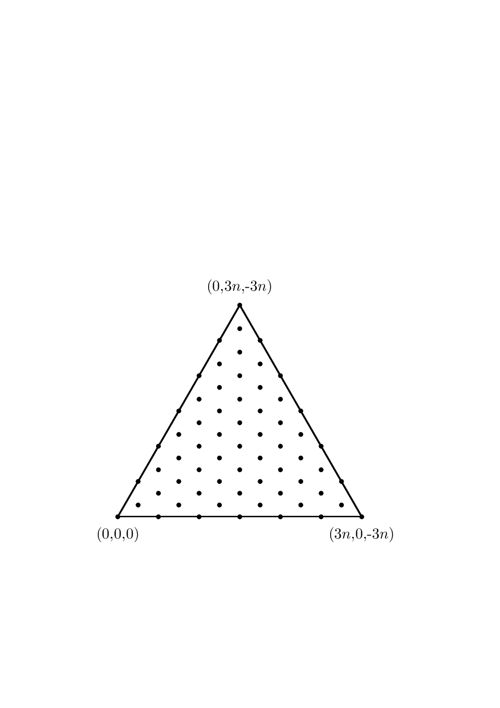
It is again convenient to use homogeneous coordinates as defined in the previous subsection. The ΩB\Omega_{B} is the regular hexagon in Fig. 1 rotated by 90∘90^{\circ}, as depicted in Figure 2, in which the right hand figure is labeled in homogeneous coordinates.

Figure 5. The hexagon domain and ΩB\Omega_{B}

Here the index set ΛN†={k∈ℤ2:−n≤2k2+k1,k2−k1,2k1+k2<n}\Lambda_{N}^{\dagger}=\left\{k\in{\mathbb{Z}}^{2}:\ -n\leq 2k_{2}+k_{1},k_{2}-k_{1},2k_{1}+k_{2}<n\right\}, which becomes in homogeneous coordinates 𝕂n†{\mathbb{K}}_{n}^{\dagger} defined by

𝕂n†:={𝐣∈ℍ:−n≤j2−j1,j1−j3,j2−j3<n}.\displaystyle{\mathbb{K}}_{n}^{{\dagger}}:=\{{\mathbf{j}}\in{\mathbb{H}}:-n\leq j_{2}-j_{1},j_{1}-j_{3},j_{2}-j_{3}<n\}.

We also have ΛN={k∈ℤ2:−n≤2k2−k1,k1+k2,2k1−k2<n}\Lambda_{N}=\left\{k\in{\mathbb{Z}}^{2}:\ -n\leq 2k_{2}-k_{1},k_{1}+k_{2},2k_{1}-k_{2}<n\right\}. Recall that 𝐭≡0(mod3){\mathbf{t}}\equiv 0\pmod{3} means, by definition, t1≡t2≡t3(mod3)t_{1}\equiv t_{2}\equiv t_{3}\pmod{3}. It is not hard to see that the set ΛN\Lambda_{N} becomes, in homogeneous coordinates, 𝕂n{\mathbb{K}}_{n} defined by

𝕂n:={𝐣∈ℍ:−n≤j1,j2,−j3<n,𝐣≡0(mod3)}.\displaystyle{\mathbb{K}}_{n}:=\{{\mathbf{j}}\in{\mathbb{H}}:-n\leq j_{1},j_{2},-j_{3}<n,\ {\mathbf{j}}\equiv 0\pmod{3}\}.

We also denote by 𝕂n†⁣∗{\mathbb{K}}_{n}^{{\dagger}*} and 𝕂n∗{\mathbb{K}}_{n}^{*} the sets defined with ≤\leq in place of << in 𝕂n†{\mathbb{K}}_{n}^{\dagger} and 𝕂n{\mathbb{K}}_{n}, respectively. The set 𝕂n∗{\mathbb{K}}_{n}^{*} can be obtained form a rotation of 𝕂n†⁣∗{\mathbb{K}}_{n}^{{\dagger}*}, as shown in the following proposition, which can be easily verified.

Proposition 3.5.

For 𝐤=(k1,k2,k3)∈ℍ{\mathbf{k}}=(k_{1},k_{2},k_{3})\in{\mathbb{H}}, define 𝐤^:=(k3−k2,k1−k3,k2−k1)\widehat{{\mathbf{k}}}:=(k_{3}-k_{2},k_{1}-k_{3},k_{2}-k_{1}). Then 𝐤^3∈𝕂n†⁣∗\frac{\widehat{\mathbf{k}}}{3}\in{\mathbb{K}}_{n}^{{\dagger}*} if 𝐤∈𝕂n∗{\mathbf{k}}\in{\mathbb{K}}_{n}^{*} and 𝐤^∈𝕂n∗\widehat{\mathbf{k}}\in{\mathbb{K}}_{n}^{*} if 𝐤∈𝕂n†⁣∗{\mathbf{k}}\in{\mathbb{K}}_{n}^{{\dagger}*}.

The finite dimensional space ℋn{\mathcal{H}}_{n} of exponential functions becomes

𝒦n:=span⁡{ϕ𝐣​(𝐭)=e2​π​i3​𝐣𝗍𝗋​𝐭:𝐣∈𝕂n†}and𝒦n∗:=span⁡{ϕ𝐣:𝐣∈𝕂n†⁣∗}.{\mathcal{K}}_{n}:=\operatorname{span}\left\{\phi_{\mathbf{j}}({\mathbf{t}})=\mathrm{e}^{\frac{2\pi i}{3}{\mathbf{j}}^{\mathsf{tr}}{\mathbf{t}}}:{\mathbf{j}}\in{\mathbb{K}}_{n}^{{\dagger}}\right\}\quad\hbox{and}\quad{\mathcal{K}}_{n}^{*}:=\operatorname{span}\left\{\phi_{\mathbf{j}}:{\mathbf{j}}\in{\mathbb{K}}_{n}^{{\dagger}*}\right\}.

By induction, it follows that dim𝒦n=|𝕂n|=n2\dim{\mathcal{K}}_{n}=|{\mathbb{K}}_{n}|=n^{2} and dim𝒦n∗=|𝕂n∗|=n2+n+1\dim{\mathcal{K}}_{n}^{*}=|{\mathbb{K}}_{n}^{*}|=n^{2}+n+1 if n=0,2(mod3)n=0,2\pmod{3} and |𝕂n∗|=n2+n−1|{\mathbb{K}}_{n}^{*}|=n^{2}+n-1 if n=1(mod3)n=1\pmod{3}.

Refer to caption
Refer to caption
Figure 6. The set 𝕂3​n∗{\mathbb{K}}^{*}_{3n} (left) and the set 𝕂3​n†⁣∗{\mathbb{K}}^{{\dagger}*}_{3n} (right).

The two sets 𝕂3​n∗{\mathbb{K}}_{3n}^{*} and 𝕂3​n†⁣∗{\mathbb{K}}_{3n}^{{\dagger}*} take different shapes, which we depict in Figure 6. Define

(3.17) ⟨f,g⟩n:=1n2​∑𝐣∈𝕂nf⁡(𝐣n)​f⁡(𝐣n)¯and⟨f,g⟩n∗=1n2​∑𝐣∈𝕂n∗c𝐣(n)​f​(𝐣n)​f⁡(𝐣n)¯,\langle f,g\rangle_{n}:=\frac{1}{n^{2}}\sum_{{\mathbf{j}}\in{\mathbb{K}}_{n}}f(\tfrac{{\mathbf{j}}}{n})\overline{f(\tfrac{{\mathbf{j}}}{n})}\quad\hbox{and}\quad\langle f,g\rangle_{n}^{*}=\frac{1}{n^{2}}\sum_{{\mathbf{j}}\in{\mathbb{K}}_{n}^{*}}c_{{\mathbf{j}}}^{(n)}f(\tfrac{{\mathbf{j}}}{n})\overline{f(\tfrac{{\mathbf{j}}}{n})},

where c𝐣(n)c_{{\mathbf{j}}}^{(n)} are as defined in (3.9) with ℍn{\mathbb{H}}_{n} replaced by 𝕂n{\mathbb{K}}_{n}.

Theorem 3.6.

For n≥0n\geq 0, 1|Ω|​∫Ωf⁡(x)​g⁡(x)¯​𝑑x=⟨f,g⟩n=⟨f,g⟩n∗\frac{1}{|\Omega|}\int_{\Omega}f(x)\overline{g(x)}dx=\langle f,g\rangle_{n}=\langle f,g\rangle_{n}^{*} for f,g∈𝒦nf,g\in{\mathcal{K}}_{n}. In particular, ⟨ϕ𝐣,ϕ𝐤⟩n∗=1\langle\phi_{\mathbf{j}},\phi_{\mathbf{k}}\rangle_{n}^{*}=1 if 𝐣^≡𝐤^(mod3​n)\hat{\mathbf{j}}\equiv\hat{\mathbf{k}}\pmod{3n} and ⟨ϕ𝐣,ϕ𝐤⟩n∗=0\langle\phi_{\mathbf{j}},\phi_{\mathbf{k}}\rangle_{n}^{*}=0 otherwise, for 𝐤,𝐣∈𝕂n{\mathbf{k}},{\mathbf{j}}\in{\mathbb{K}}_{n}. Moreover, we have the cubature

(3.18) 1|Ω|​∫Ωf⁡(𝐭)​𝑑𝐭=1n2​∑𝐣∈𝒦n∗c𝐣(n)​f​(𝐣n),∀f∈𝒦2​n−1∗.\displaystyle\frac{1}{|\Omega|}\int_{\Omega}f({\mathbf{t}})d{\mathbf{t}}=\frac{1}{n^{2}}\sum_{{\mathbf{j}}\in{\mathcal{K}}_{n}^{*}}c_{\mathbf{j}}^{(n)}f(\tfrac{{\mathbf{j}}}{n}),\quad\forall f\in{\mathcal{K}}_{2n-1}^{*}.

The part of the theorem on ⟨f,g⟩n\langle f,g\rangle_{n} is exactly Theorem 2.2, while the part on ⟨f,g⟩n∗\langle f,g\rangle_{n}^{*} and the cubature can be proved by periodicity, just like the proof of Theorem 3.3 in [7], upon using the Proposition 3.5. The cubature (3.18) is already one in Stage 2; we can also derive a cubature with nodes indexed by 𝕂n{\mathbb{K}}_{n} as in Stage 1.

Next we consider the invariant and anti-invariant functions under 𝒜2{\mathcal{A}}_{2}, which are the generalized cosines 𝖳𝖢𝐤{\mathsf{TC}}_{\mathbf{k}} and the generalized sines 𝖳𝖲𝐤{\mathsf{TS}}_{\mathbf{k}} considered in the previous subsection. By restricting to such functions, we again obtain cubature on the triangle Δ\Delta. The index set of the nodes of the cubature, denoted by Υ\Upsilon, is

Υn:={𝐣∈ℍ:0≤j1,j2,−j3≤n,𝐣≡0(mod3)}\displaystyle\Upsilon_{n}:=\{{\mathbf{j}}\in{\mathbb{H}}:0\leq j_{1},j_{2},-j_{3}\leq n,{\mathbf{j}}\equiv 0\pmod{3}\}

derived by symmetry from 𝕂n∗{\mathbb{K}}_{n}^{*}, whereas the index set of the invariant functions being integrated exactly by the cubature, denoted by Υ†\Upsilon^{\dagger}, is derived from 𝕂n†⁣∗{\mathbb{K}}_{n}^{{\dagger}*},

Υn†={𝐣∈ℍ:0≤j1,j2,−j3≤n,j2−j3≤n,j1−j3≤n},\displaystyle\Upsilon_{n}^{\dagger}=\{{\mathbf{j}}\in{\mathbb{H}}:0\leq j_{1},j_{2},-j_{3}\leq n,j_{2}-j_{3}\leq n,j_{1}-j_{3}\leq n\},

which is inside a quadrilateral; Figure 7 shows its relative position in ΩB\Omega_{B}.

Figure 7. The fundamental quadrilateral of ΩB\Omega_{B} under 𝒜2{\mathcal{A}}_{2}

We define the following subspaces of trigonometric functions,

𝒯​Cn=span⁡{𝖳𝖢𝐤:𝐤∈Υn†}and𝒯​Sn=span⁡{𝖳𝖲𝐤:𝐤∈Υn†⁣∘}.{\mathcal{T}\!C}_{n}=\operatorname{span}\{{\mathsf{TC}}_{\mathbf{k}}:{\mathbf{k}}\in\Upsilon_{n}^{\dagger}\}\quad\hbox{and}\quad{\mathcal{T}\!S}_{n}=\operatorname{span}\{{\mathsf{TS}}_{\mathbf{k}}:{\mathbf{k}}\in\Upsilon_{n}^{{\dagger}\circ}\}.

The set Υn\Upsilon_{n} takes a symmetric form when nn is a multiple of 33. In Figure (8) we depict the index sets Υ3​n\Upsilon_{3n} and Υ3​n†\Upsilon_{3n}^{\dagger}.

Refer to caption
Refer to caption
Figure 8. the index sets Υ3​n\Upsilon_{3n} (left) and Υ3​n†\Upsilon_{3n}^{{\dagger}} (right).
Theorem 3.7.

The following cubature is exact for all f∈𝒯​C2​n−1f\in{\mathcal{T}\!C}_{2n-1},

(3.19) 1|Δ|​∫Δf⁡(𝐭)​𝑑𝐭=1n2​∑𝐣∈Υnλ𝐣(n)​f​(𝐣n),λ𝐣(n):={6,𝐣∈Υn∘,3,𝐣∈Υne,1,𝐣∈Υnv.\displaystyle\frac{1}{|\Delta|}\int_{\Delta}f({\mathbf{t}})d{\mathbf{t}}=\frac{1}{n^{2}}\sum_{{\mathbf{j}}\in\Upsilon_{n}}\lambda_{{\mathbf{j}}}^{(n)}f(\tfrac{{\mathbf{j}}}{n}),\qquad\lambda_{\mathbf{j}}^{(n)}:=\begin{cases}6,&{\mathbf{j}}\in\Upsilon^{\circ}_{n},\\ 3,&{\mathbf{j}}\in\Upsilon^{\mathrm{e}}_{n},\\ 1,&{\mathbf{j}}\in\Upsilon^{\mathrm{v}}_{n}.\end{cases}

The formula (3.19) is derived from (3.18) by using the invariance of the functions in 𝒯​C2​n−1{\mathcal{T}\!C}_{2n-1} and the fact Ω=(∪σ∈𝒜2{𝐭σ:𝐭∈Δ∘})∪(∪σ∈𝒜2{𝐭σ:𝐭∈∂Δ})\Omega=\big(\cup_{\sigma\in{\mathcal{A}}_{2}}\{{\mathbf{t}}\sigma:{\mathbf{t}}\in\Delta^{\circ}\}\big)\cup\big(\cup_{\sigma\in{\mathcal{A}}_{2}}\{{\mathbf{t}}\sigma:{\mathbf{t}}\in\partial\Delta\}\big). As the proof is similar to that of (3.14) in [7], we shall omit the details.

Similarly, we can also derive a cubature for 𝒯​S2​n−1{\mathcal{T}\!S}_{2n-1} based on points in Υn∘\Upsilon_{n}^{\circ}. These are cubature in Stage 3. We note that the set of nodes in (3.19) is different from that in (3.14), see Figure 2 and Figure 8, even though both are on the triangle.

As in the case of Hexagon-Hexagon, we can continue to Stage 4, where the cubature (3.19) is mapped by the change of variables (3.15) to an algebraic cubature for w−1/2(x,y)dxdyw_{-1/2}(x,y)dxdy on Δ∗\Delta^{*}, the region bounded by SteinerÕs hypocycloid, which is a cubature exact for all polynomials in Π2​n−12\Pi_{2n-1}^{2} but with many more nodes than the one derived in the Hexagon-Hexagon case.

The set of cubature points in (3.19) and its image in the region bounded by Steiner’s hypocycloid have also been studied in [15].

3.5.2. Interpolation

Applying Theorem 2.3 to the current set up, we obtain an interpolation operator ℐn​f{\mathcal{I}}_{n}f that interpolates ff on 𝕂n{\mathbb{K}}_{n} in the hexagon. We would like to consider interpolation on the triangle based on points in Υn\Upsilon_{n}. For this purpose, we first construct a near interpolation operator on the symmetric set of points 𝕂n∗{\mathbb{K}}_{n}^{*}.

Theorem 3.8.

Let 𝒮𝐣:={𝐤∈𝕂n∗:𝐤≡𝐣(mod3​n)}.{\mathcal{S}}_{\mathbf{j}}:=\left\{{\mathbf{k}}\in{\mathbb{K}}_{n}^{*}:{\mathbf{k}}\equiv{\mathbf{j}}\pmod{3n}\right\}. For f∈C⁡(Ω)f\in C(\Omega), define

ℐn∗​f​(𝐭):=∑𝐣∈𝕂n∗f⁡(𝐣n)​Φn​(𝐭−𝐣n),Φn​(𝐭):=1n2​∑𝐣∈𝕂n†⁣∗c𝐣^(n)​ϕ𝐣​(𝐭).{\mathcal{I}}_{n}^{*}f({\mathbf{t}}):=\sum_{{\mathbf{j}}\in{\mathbb{K}}_{n}^{*}}f(\tfrac{{\mathbf{j}}}{n})\Phi_{n}({\mathbf{t}}-\tfrac{{\mathbf{j}}}{n}),\quad\Phi_{n}({\mathbf{t}}):=\frac{1}{n^{2}}\sum_{{\mathbf{j}}\in{\mathbb{K}}_{n}^{{\dagger}*}}c_{\widehat{\mathbf{j}}}^{(n)}\phi_{\mathbf{j}}({\mathbf{t}}).

Then ℐn∗​f∈𝒦n∗{\mathcal{I}}_{n}^{*}f\in{\mathcal{K}}_{n}^{*} and ℐn∗​f​(𝐣n)=f⁡(𝐣n){\mathcal{I}}_{n}^{*}f(\tfrac{{\mathbf{j}}}{n})=f(\tfrac{{\mathbf{j}}}{n}) if 𝐣∈𝕂n∘{\mathbf{j}}\in{\mathbb{K}}_{n}^{\circ}, and ℐn∗​f​(𝐣n)=∑𝐤∈𝒮𝐣f⁡(𝐤n){\mathcal{I}}_{n}^{*}f(\tfrac{{\mathbf{j}}}{n})=\sum_{{\mathbf{k}}\in{\mathcal{S}}_{\mathbf{j}}}f(\frac{{\mathbf{k}}}{n}) if 𝐣∈∂𝕂n∗{\mathbf{j}}\in\partial{\mathbb{K}}_{n}^{*}, the boundary of 𝕂n∗{\mathbb{K}}_{n}^{*}. Furthermore, Φn∗​(𝐭)\Phi_{n}^{*}({\mathbf{t}}) is a real function and it is given by the following formula when n=0(mod3)n=0\pmod{3},

(3.20) Φn​(𝐭)=\displaystyle\Phi_{n}({\mathbf{t}})= 1n2[−12∑i=13(2​cos⁡π​si+cos⁡π​ti)​sin⁡π​ti​cos⁡2​π​n​ti3sin⁡π​t1​sin⁡π​t2​sin⁡π​t3\displaystyle\frac{1}{n^{2}}\left[-\frac{1}{2}\sum_{i=1}^{3}\frac{(2\cos\pi s_{i}+\cos\pi t_{i})\sin\pi t_{i}\cos\frac{2\pi nt_{i}}{3}}{\sin\pi t_{1}\sin\pi t_{2}\sin\pi t_{3}}\right.
−13(cos2​n​π​t13+cos2​n​π​t23+cos2​n​π​s33)],\displaystyle\qquad\left.-\frac{1}{3}\big(\cos\tfrac{2n\pi t_{1}}{3}+\cos\tfrac{2n\pi t_{2}}{3}+\cos\tfrac{2n\pi s_{3}}{3}\big)\right],

where s1=t3−t23,s2=t1−t33,s3=t2−t13s_{1}=\frac{t_{3}-t_{2}}{3},s_{2}=\frac{t_{1}-t_{3}}{3},s_{3}=\frac{t_{2}-t_{1}}{3}.

Proof.

By Proposition 3.5, 𝐤∈𝕂n∗{\mathbf{k}}\in{\mathbb{K}}_{n}^{*} implies 𝐤^3∈𝕂n†⁣∗\frac{\widehat{\mathbf{k}}}{3}\in{\mathbb{K}}_{n}^{{\dagger}*}, and 𝐣∈𝕂n†⁣∗{\mathbf{j}}\in{\mathbb{K}}_{n}^{{\dagger}*} implies 𝐣^∈𝕂n∗\widehat{{\mathbf{j}}}\in{\mathbb{K}}_{n}^{*}. By homogeneity, 𝐤⋅𝐭=(k3−k2)​s1+(k1−k3)​s2+(k2−k1)​s3=𝐤^⋅𝐬{\mathbf{k}}\cdot{\mathbf{t}}=(k_{3}-k_{2})s_{1}+(k_{1}-k_{3})s_{2}+(k_{2}-k_{1})s_{3}=\widehat{\mathbf{k}}\cdot{\mathbf{s}}. As a result,

Φn​(𝐭)=1n2​∑𝐣∈𝕂n†⁣∗c𝐣^(n)​ϕ𝐣^​(𝐬)=1n2​∑𝐣∈𝕂n∗c𝐣(n)​ϕ𝐣​(𝐬).\displaystyle\Phi_{n}({\mathbf{t}})=\frac{1}{n^{2}}\sum_{{\mathbf{j}}\in{\mathbb{K}}_{n}^{{\dagger}*}}{c}_{\widehat{\mathbf{j}}}^{(n)}\phi_{\widehat{\mathbf{j}}}({\mathbf{s}})=\frac{1}{n^{2}}\sum_{{\mathbf{j}}\in{\mathbb{K}}_{n}^{*}}{c}_{{\mathbf{j}}}^{(n)}\phi_{{\mathbf{j}}}({\mathbf{s}}).

Consequently, by the definition in (3.17),

Φn​(𝐤−𝐣n)=1n2​∑𝐥∈𝕂n∗c𝐥(n)​ϕ𝐥​(𝐤^−𝐣^n)=1n2​∑𝐥∈𝕂n∗c𝐥(n)​ϕ𝐤^−𝐣^​(𝐥n)=⟨ϕ𝐤^,ϕ𝐣^⟩n∗.\displaystyle\Phi_{n}(\tfrac{{\mathbf{k}}-{\mathbf{j}}}{n})=\frac{1}{n^{2}}\sum_{{\mathbf{l}}\in{\mathbb{K}}_{n}^{*}}c_{\mathbf{l}}^{(n)}\phi_{\mathbf{l}}(\tfrac{\widehat{{\mathbf{k}}}-\widehat{{\mathbf{j}}}}{n})=\frac{1}{n^{2}}\sum_{{\mathbf{l}}\in{\mathbb{K}}_{n}^{*}}c_{\mathbf{l}}^{(n)}\phi_{\widehat{{\mathbf{k}}}-\widehat{{\mathbf{j}}}}(\tfrac{{\mathbf{l}}}{n})=\langle\phi_{\widehat{{\mathbf{k}}}},\phi_{\widehat{{\mathbf{j}}}}\rangle^{*}_{n}.

Thus, by Theorem 3.6, it follows that

(3.21) Φn​(𝐤−𝐣n)=⟨ϕ𝐤^,ϕ𝐣^⟩n∗={1,𝐤^=𝐣^+n𝐥,𝐥∈ℍ,0,otherwise,\displaystyle\begin{split}\Phi_{n}(\tfrac{{\mathbf{k}}-{\mathbf{j}}}{n})=\langle\phi_{\widehat{\mathbf{k}}},\phi_{\widehat{\mathbf{j}}}\rangle_{n}^{*}=\begin{cases}1,&\widehat{\mathbf{k}}=\widehat{\mathbf{j}}+n{\mathbf{l}},\,{\mathbf{l}}\in{\mathbb{H}},\\ 0,&\text{otherwise},\end{cases}\end{split}

which proves the stated result of ℐn∗​f{\mathcal{I}}_{n}^{*}f.

To derive the compact formula for Φn\Phi_{n} we essentially need a formula for the Dirichlet kernel, denoted by Θn​(𝐭)\Theta_{n}({\mathbf{t}}), of the Fourier series over ℍn†⁣∗{\mathbb{H}}^{{\dagger}*}_{n},

Θn​(𝐭)=∑𝐣∈ℍn†⁣∗ϕ𝐣​(𝐭).\displaystyle\Theta_{n}({\mathbf{t}})=\sum_{{\mathbf{j}}\in{\mathbb{H}}^{{\dagger}*}_{n}}\phi_{{\mathbf{j}}}({\mathbf{t}}).

Indeed, by the definition of c𝐣(n)c_{\mathbf{j}}^{(n)}, it follows that

(3.22) n2​Φn​(𝐭)=12​(Θn​(𝐭)+Θn−1​(𝐭))−{𝖳𝖢n3,n3,−2​n3​(𝐭),n≡0(mod3),0,o​t​h​e​r​w​i​s​e.\displaystyle n^{2}{\Phi}_{n}({\mathbf{t}})=\frac{1}{2}\big({\Theta}_{n}({\mathbf{t}})+{\Theta}_{n-1}({\mathbf{t}})\big)-\begin{cases}{\mathsf{TC}}_{\frac{n}{3},\frac{n}{3},-\frac{2n}{3}}({\mathbf{t}}),&n\equiv 0\pmod{3},\\ 0,&otherwise.\end{cases}

Using the identity 𝐤⋅𝐭=𝐤^⋅𝐬{\mathbf{k}}\cdot{\mathbf{t}}=\widehat{\mathbf{k}}\cdot{\mathbf{s}} and Proposition 3.5, we derive that

Θn​(𝐭)=∑𝐤∈𝕂n†⁣∗ϕ𝐤​(𝐭)=∑𝐤∈𝕂n†⁣∗ϕ𝐤^​(𝐬)=∑𝐣∈𝕂n∗ϕ𝐣​(𝐬).\displaystyle{\Theta}_{n}({\mathbf{t}})=\sum_{{\mathbf{k}}\in{\mathbb{K}}_{n}^{{\dagger}*}}\phi_{\mathbf{k}}({\mathbf{t}})=\sum_{{\mathbf{k}}\in{\mathbb{K}}_{n}^{{\dagger}*}}\phi_{\widehat{\mathbf{k}}}({\mathbf{s}})=\sum_{{\mathbf{j}}\in{\mathbb{K}}_{n}^{*}}\phi_{{\mathbf{j}}}({\mathbf{s}}).

We now partition 𝕂n∗{\mathbb{K}}_{n}^{*} into three parts according to the congruence relation,

𝕂n(0):={𝐣∈𝕂n∗:j1≡j2≡j3≡0(mod3)},\displaystyle{\mathbb{K}}_{n}^{(0)}:=\big\{{\mathbf{j}}\in{{\mathbb{K}}}_{n}^{*}:j_{1}\equiv j_{2}\equiv j_{3}\equiv 0\pmod{3}\big\},
𝕂n(1):={𝐣∈𝕂n∗:j1≡j2≡j3≡1(mod3)},\displaystyle{\mathbb{K}}_{n}^{(1)}:=\big\{{\mathbf{j}}\in{{\mathbb{K}}}_{n}^{*}:j_{1}\equiv j_{2}\equiv j_{3}\equiv 1\pmod{3}\big\},
𝕂n(2):={𝐣∈𝕂n∗:j1≡j2≡j3≡2(mod3)}.\displaystyle{\mathbb{K}}_{n}^{(2)}:=\big\{{\mathbf{j}}\in{{\mathbb{K}}}_{n}^{*}:j_{1}\equiv j_{2}\equiv j_{3}\equiv 2\pmod{3}\big\}.

Using the fact that 𝐣∈𝕂n(0)⟺𝐣3∈ℍ⌊n3⌋∗{\mathbf{j}}\in{\mathbb{K}}_{n}^{(0)}\Longleftrightarrow\frac{{\mathbf{j}}}{3}\in{\mathbb{H}}_{\lfloor\frac{n}{3}\rfloor}^{*}, where ℍn∗{\mathbb{H}}_{n}^{*} is the index defined in the previous subsection, and ϕ𝐣​(𝐬)=ϕ𝐣3​(3​𝐬)\phi_{{\mathbf{j}}}({\mathbf{s}})=\phi_{\frac{{\mathbf{j}}}{3}}(3{\mathbf{s}}) if 𝐣∈𝕂n(0){\mathbf{j}}\in{\mathbb{K}}_{n}^{(0)}, we obtain from the Dirichlet kernel over ℍn∗{\mathbb{H}}_{n}^{*} in (3.10) of [7],

(3.23) ∑𝐣∈𝕂n(0)ϕ𝐣​(𝐬)=∏j=13sin⁡π​⌊n+33⌋​tjsin⁡π​tj−∏j=13sin⁡π​⌊n3⌋​tjsin⁡π​tj=∑j=13sin⁡2​π​⌊n3⌋​tj−sin⁡2​π​⌊n+33⌋​tj4​sin⁡π​t1​sin⁡π​t2​sin⁡π​t3,\displaystyle\begin{split}\sum_{{\mathbf{j}}\in{\mathbb{K}}_{n}^{(0)}}\phi_{{\mathbf{j}}}({\mathbf{s}})&=\prod_{j=1}^{3}\frac{\sin\pi\lfloor\frac{n+3}{3}\rfloor t_{j}}{\sin\pi t_{j}}-\prod_{j=1}^{3}\frac{\sin\pi\lfloor\frac{n}{3}\rfloor t_{j}}{\sin\pi t_{j}}\\ &=\sum_{j=1}^{3}\frac{\sin 2\pi\lfloor\frac{n}{3}\rfloor t_{j}-\sin 2\pi\lfloor\frac{n+3}{3}\rfloor t_{j}}{4\sin\pi t_{1}\sin\pi t_{2}\sin\pi t_{3}},\end{split}

where we have used the identity sin2t1+sin2t2+sin2t3=−4sint1sint2sint3\sin 2t_{1}+\sin 2t_{2}+\sin 2t_{3}=-4\sin t_{1}\sin t_{2}\sin t_{3} in the last equal sign [7, (3.15)]. Next we note that 𝕂n(1){\mathbb{K}}_{n}^{(1)} can be divided into the following three (non-overlapping) subsets 𝕂n(1)=𝕂n(1,3)∪𝕂n(1,2)∪𝕂n(1,1){\mathbb{K}}_{n}^{(1)}={\mathbb{K}}_{n}^{(1,3)}\cup{\mathbb{K}}_{n}^{(1,2)}\cup{\mathbb{K}}_{n}^{(1,1)}, where

𝕂n(1,1)={(−j2−j3,j2,j3):j2≡j3≡1(mod3), 1≤j2,−j3≤n},\displaystyle{\mathbb{K}}_{n}^{(1,1)}=\left\{(-j_{2}-j_{3},j_{2},j_{3}):j_{2}\equiv j_{3}\equiv 1\pmod{3},\ 1\leq j_{2},-j_{3}\leq n\right\},
𝕂n(1,2)={(j1,−j1−j3,j3):j3≡j1≡1(mod3), 1≤j3,−j1≤n},\displaystyle{\mathbb{K}}_{n}^{(1,2)}=\left\{(j_{1},-j_{1}-j_{3},j_{3}):j_{3}\equiv j_{1}\equiv 1\pmod{3},\ 1\leq j_{3},-j_{1}\leq n\right\},
𝕂n(1,3)={(j1,j2,−j1−j2):j1≡j2≡1(mod3), 1≤j1,−j2≤n}.\displaystyle{\mathbb{K}}_{n}^{(1,3)}=\left\{(j_{1},j_{2},-j_{1}-j_{2}):j_{1}\equiv j_{2}\equiv 1\pmod{3},\ 1\leq j_{1},-j_{2}\leq n\right\}.

Using the last set 𝕂n(1,3){\mathbb{K}}_{n}^{(1,3)}, we define

(3.24) ℐ⁡(t1,t2):=∑𝐣∈𝕂n(1,3)ϕ𝐣​(𝐬)=∑1≤j1≤n3|j1−1∑1≤−j2≤n3|j2−1e2​i​π3​(j2​t1−j1​t2)=e−2​i​π​t23​(1−e−2​i​π​⌊n+23⌋​t2)1−e−2​i​π​t2​e−4​i​π​t13​(1−e−2​i​π​⌊n+13⌋​t1)1−e−2​i​π​t1=(e−2​i​π​s2−e−2​i​π​s1)​(1−e−2​i​π​⌊n+13⌋​t1)​(1−e−2​i​π​⌊n+23⌋​t2)(1−e−2​i​π​t1)​(1−e−2​i​π​t2)​(1−e−2​i​π​t3),\displaystyle\begin{split}{\mathcal{I}}(t_{1},t_{2}):=&\ \sum_{{\mathbf{j}}\in{\mathbb{K}}_{n}^{(1,3)}}\phi_{{\mathbf{j}}}({\mathbf{s}})=\sum_{1\leq j_{1}\leq n\atop 3|j_{1}-1}\sum_{1\leq-j_{2}\leq n\atop 3|j_{2}-1}\mathrm{e}^{\frac{2i\pi}{3}(j_{2}t_{1}-j_{1}t_{2})}\\ =&\ \frac{\mathrm{e}^{-\frac{2i\pi t_{2}}{3}}(1-\mathrm{e}^{-2i\pi\lfloor\frac{n+2}{3}\rfloor t_{2}})}{1-\mathrm{e}^{-2i\pi t_{2}}}\frac{\mathrm{e}^{-\frac{4i\pi t_{1}}{3}}(1-\mathrm{e}^{-2i\pi\lfloor\frac{n+1}{3}\rfloor t_{1}})}{1-\mathrm{e}^{-2i\pi t_{1}}}\\ =&\ \frac{(\mathrm{e}^{-2i\pi s_{2}}-\mathrm{e}^{-2i\pi s_{1}})(1-\mathrm{e}^{-2i\pi\lfloor\frac{n+1}{3}\rfloor t_{1}})(1-\mathrm{e}^{-2i\pi\lfloor\frac{n+2}{3}\rfloor t_{2}})}{(1-\mathrm{e}^{-2i\pi t_{1}})(1-\mathrm{e}^{-2i\pi t_{2}})(1-\mathrm{e}^{-2i\pi t_{3}})},\end{split}

where the second equal sign follows from 𝐣⋅𝐬=j1​(s1−s3)+j2​(s2−s3)=j2​t1−j1​t2{\mathbf{j}}\cdot{\mathbf{s}}=j_{1}(s_{1}-s_{3})+j_{2}(s_{2}-s_{3})=j_{2}t_{1}-j_{1}t_{2}. Moreover, we have 𝐣⋅𝐬=j2​t1−j1​t2=j3​t2−j2​t3=j1​t3−j3​t1{\mathbf{j}}\cdot{\mathbf{s}}=j_{2}t_{1}-j_{1}t_{2}=j_{3}t_{2}-j_{2}t_{3}=j_{1}t_{3}-j_{3}t_{1}, which yields

ℐ⁡(t2,t3)=∑𝐣∈𝕂n(1,1)ϕ𝐣​(𝐬)andℐ⁡(t3,t1)=∑𝐣∈𝕂n(1,2)ϕ𝐣​(𝐬).\displaystyle{\mathcal{I}}(t_{2},t_{3})=\sum_{{\mathbf{j}}\in{\mathbb{K}}_{n}^{(1,1)}}\phi_{{\mathbf{j}}}({\mathbf{s}})\quad\hbox{and}\quad{\mathcal{I}}(t_{3},t_{1})=\sum_{{\mathbf{j}}\in{\mathbb{K}}_{n}^{(1,2)}}\phi_{{\mathbf{j}}}({\mathbf{s}}).

As a result, we conclude

∑𝐣∈𝕂n(1)ϕ𝐣​(𝐬)=ℐ⁡(t1,t2)+ℐ⁡(t2,t3)+ℐ⁡(t3,t1).\displaystyle\sum_{{\mathbf{j}}\in{\mathbb{K}}_{n}^{(1)}}\phi_{{\mathbf{j}}}({\mathbf{s}})={\mathcal{I}}(t_{1},t_{2})+{\mathcal{I}}(t_{2},t_{3})+{\mathcal{I}}(t_{3},t_{1}).

Furthermore, we note that 𝕂n(2)={−𝐣:𝐣∈𝕂n(1)}{\mathbb{K}}_{n}^{(2)}=\left\{-{\mathbf{j}}:{\mathbf{j}}\in{\mathbb{K}}_{n}^{(1)}\right\} and, consequently,

∑𝐣∈𝕂n(1)∪𝕂n(2)ϕ𝐣​(𝐬)\displaystyle\sum_{{\mathbf{j}}\in{\mathbb{K}}_{n}^{(1)}\cup{\mathbb{K}}_{n}^{(2)}}\phi_{{\mathbf{j}}}({\mathbf{s}}) =∑𝐣∈𝕂n(1)ϕ𝐣​(𝐬)+∑𝐣∈𝕂n(2)ϕ𝐣​(𝐬)=∑𝐣∈𝕂n(1)ϕ𝐣​(𝐬)+∑𝐣∈𝕂n(1)ϕ𝐣​(−𝐬)\displaystyle=\sum_{{\mathbf{j}}\in{\mathbb{K}}_{n}^{(1)}}\phi_{{\mathbf{j}}}({\mathbf{s}})+\sum_{{\mathbf{j}}\in{\mathbb{K}}_{n}^{(2)}}\phi_{{\mathbf{j}}}({\mathbf{s}})=\sum_{{\mathbf{j}}\in{\mathbb{K}}_{n}^{(1)}}\phi_{{\mathbf{j}}}({\mathbf{s}})+\sum_{{\mathbf{j}}\in{\mathbb{K}}_{n}^{(1)}}\phi_{{\mathbf{j}}}(-{\mathbf{s}})
=∑𝐣∈𝕂n(1)ϕ𝐣​(𝐬)+∑𝐣∈𝕂n(1)ϕ𝐣​(𝐬)¯=2​ℜ⁡{ℐ⁡(t1,t2)+ℐ⁡(t2,t3)+ℐ⁡(t3,t1)}.\displaystyle=\sum_{{\mathbf{j}}\in{\mathbb{K}}_{n}^{(1)}}\phi_{{\mathbf{j}}}({\mathbf{s}})+\sum_{{\mathbf{j}}\in{\mathbb{K}}_{n}^{(1)}}\overline{\phi_{{\mathbf{j}}}({\mathbf{s}})}=2\Re\{{\mathcal{I}}(t_{1},t_{2})+{\mathcal{I}}(t_{2},t_{3})+{\mathcal{I}}(t_{3},t_{1})\}.

Now assume that nn is a multiple of 33. By using (3.24) and the fact that 𝐭{\mathbf{t}} is homogeneous, we obtain

∑𝐣∈𝕂n(1)∪𝕂n(2)ϕ𝐣​(𝐬)=2​ℜ{ℐ(t1,t2))+2ℜ(ℐ(t2,t3))+2ℜ(ℐ(t3,t1)}=2​ℜ{(e−2​i​π​s2−e−2​i​π​s1)​(1+e2​i​π​n3​t3−e−2​i​π​n3​t1−e−2​i​π​n3​t2)(1−e−2​i​π​t1)​(1−e−2​i​π​t2)​(1−e−2​i​π​t3)+(e−2​i​π​s3−e−2​i​π​s2)​(1+e2​i​π​n3​t1−e−2​i​π​n3​t2−e−2​i​π​n3​t3)(1−e−2​i​π​t1)​(1−e−2​i​π​t2)​(1−e−2​i​π​t3)+(e−2​i​π​s1−e−2​i​π​s3)​(1+e2​i​π​n3​t2−e−2​i​π​n3​t3−e−2​i​π​n3​t1)(1−e−2​i​π​t1)​(1−e−2​i​π​t2)​(1−e−2​i​π​t3)}.\displaystyle\begin{split}\sum_{{\mathbf{j}}\in{\mathbb{K}}_{n}^{(1)}\cup{\mathbb{K}}_{n}^{(2)}}\phi_{{\mathbf{j}}}({\mathbf{s}})=2\Re&\{{\mathcal{I}}(t_{1},t_{2}))+2\Re({\mathcal{I}}(t_{2},t_{3}))+2\Re({\mathcal{I}}(t_{3},t_{1})\}\\ =2\Re&\left\{\frac{(\mathrm{e}^{-2i\pi s_{2}}-\mathrm{e}^{-2i\pi s_{1}})(1+\mathrm{e}^{2i\pi\frac{n}{3}t_{3}}-\mathrm{e}^{-2i\pi\frac{n}{3}t_{1}}-\mathrm{e}^{-2i\pi\frac{n}{3}t_{2}})}{(1-\mathrm{e}^{-2i\pi t_{1}})(1-\mathrm{e}^{-2i\pi t_{2}})(1-\mathrm{e}^{-2i\pi t_{3}})}\right.\\ &+\frac{(\mathrm{e}^{-2i\pi s_{3}}-\mathrm{e}^{-2i\pi s_{2}})(1+\mathrm{e}^{2i\pi\frac{n}{3}t_{1}}-\mathrm{e}^{-2i\pi\frac{n}{3}t_{2}}-\mathrm{e}^{-2i\pi\frac{n}{3}t_{3}})}{(1-\mathrm{e}^{-2i\pi t_{1}})(1-\mathrm{e}^{-2i\pi t_{2}})(1-\mathrm{e}^{-2i\pi t_{3}})}\\ &\left.+\frac{(\mathrm{e}^{-2i\pi s_{1}}-\mathrm{e}^{-2i\pi s_{3}})(1+\mathrm{e}^{2i\pi\frac{n}{3}t_{2}}-\mathrm{e}^{-2i\pi\frac{n}{3}t_{3}}-\mathrm{e}^{-2i\pi\frac{n}{3}t_{1}})}{(1-\mathrm{e}^{-2i\pi t_{1}})(1-\mathrm{e}^{-2i\pi t_{2}})(1-\mathrm{e}^{-2i\pi t_{3}})}\right\}.\end{split}

Combining the numerators and collecting the terms in 11, e2iπn3⋅\mathrm{e}^{2i\pi\frac{n}{3}\cdot} and e−2iπn3⋅\mathrm{e}^{-2i\pi\frac{n}{3}\cdot}, we obtain that the combined numerator is equal to

(e−2​i​π​s2−e−2​i​π​s1)+(e−2​i​π​s3−e−2​i​π​s2)+(e−2​i​π​s1−e−2​i​π​s3)+(e−2​i​π​s2−e−2​i​π​s1)​e2​i​π​n3​t3−((e−2​i​π​s3−e−2​i​π​s2)+(e−2​i​π​s1−e−2​i​π​s3))​e−2​i​π​n3​t3+(e−2​i​π​s3−e−2​i​π​s2)​e2​i​π​n3​t1−((e−2​i​π​s1−e−2​i​π​s3)+(e−2​i​π​s2−e−2​i​π​s1))​e−2​i​π​n3​t1+(e−2​i​π​s1−e−2​i​π​s3)​e2​i​π​n3​t2−((e−2​i​π​s2−e−2​i​π​s1)+(e−2​i​π​s3−e−2​i​π​s2))​e−2​i​π​n3​t2=(e−2​i​π​s2−e−2​i​π​s1)​(e2​i​π​n3​t3+e−2​i​π​n3​t3)+(e−2​i​π​s3−e−2​i​π​s2)​(e2​i​π​n3​t1+e2​i​π​n3​t1)+(e−2​i​π​s1−e−2​i​π​s3)​(e2​i​π​n3​t2+e−2​i​π​n3​t2)= 2​cos⁡2​π​n​t33​ei​π​s3​(ei​π​t3−e−i​π​t3)+2​cos⁡2​π​n​t13​ei​π​s1​(ei​π​t1−e−i​π​t1)+2​cos⁡2​π​n​t23​ei​π​s2​(ei​π​t2−e−i​π​t2)= 4​i​ei​π​s3​cos⁡2​π​n​t33​sin⁡π​t3+4​i​ei​π​s1​cos⁡2​π​n​t13​sin⁡π​t1+4​i​ei​π​s2​cos⁡2​π​n​t23​sin⁡π​t2,\displaystyle\begin{split}&\ (\mathrm{e}^{-2i\pi s_{2}}-\mathrm{e}^{-2i\pi s_{1}})+(\mathrm{e}^{-2i\pi s_{3}}-\mathrm{e}^{-2i\pi s_{2}})+(\mathrm{e}^{-2i\pi s_{1}}-\mathrm{e}^{-2i\pi s_{3}})\\ &+(\mathrm{e}^{-2i\pi s_{2}}-\mathrm{e}^{-2i\pi s_{1}})\mathrm{e}^{2i\pi\frac{n}{3}t_{3}}-\big((\mathrm{e}^{-2i\pi s_{3}}-\mathrm{e}^{-2i\pi s_{2}})+(\mathrm{e}^{-2i\pi s_{1}}-\mathrm{e}^{-2i\pi s_{3}})\big)\mathrm{e}^{-2i\pi\frac{n}{3}t_{3}}\\ &+(\mathrm{e}^{-2i\pi s_{3}}-\mathrm{e}^{-2i\pi s_{2}})\mathrm{e}^{2i\pi\frac{n}{3}t_{1}}-\big((\mathrm{e}^{-2i\pi s_{1}}-\mathrm{e}^{-2i\pi s_{3}})+(\mathrm{e}^{-2i\pi s_{2}}-\mathrm{e}^{-2i\pi s_{1}})\big)\mathrm{e}^{-2i\pi\frac{n}{3}t_{1}}\\ &+(\mathrm{e}^{-2i\pi s_{1}}-\mathrm{e}^{-2i\pi s_{3}})\mathrm{e}^{2i\pi\frac{n}{3}t_{2}}-\big((\mathrm{e}^{-2i\pi s_{2}}-\mathrm{e}^{-2i\pi s_{1}})+(\mathrm{e}^{-2i\pi s_{3}}-\mathrm{e}^{-2i\pi s_{2}})\big)\mathrm{e}^{-2i\pi\frac{n}{3}t_{2}}\\ =&\ (\mathrm{e}^{-2i\pi s_{2}}-\mathrm{e}^{-2i\pi s_{1}})(\mathrm{e}^{2i\pi\frac{n}{3}t_{3}}+\mathrm{e}^{-2i\pi\frac{n}{3}t_{3}})+(\mathrm{e}^{-2i\pi s_{3}}-\mathrm{e}^{-2i\pi s_{2}})(\mathrm{e}^{2i\pi\frac{n}{3}t_{1}}+\mathrm{e}^{2i\pi\frac{n}{3}t_{1}})\\ &+(\mathrm{e}^{-2i\pi s_{1}}-\mathrm{e}^{-2i\pi s_{3}})(\mathrm{e}^{2i\pi\frac{n}{3}t_{2}}+\mathrm{e}^{-2i\pi\frac{n}{3}t_{2}})\\ =&\ 2\cos\tfrac{2\pi nt_{3}}{3}\mathrm{e}^{i\pi s_{3}}(\mathrm{e}^{i\pi t_{3}}-\mathrm{e}^{-i\pi t_{3}})+2\cos\tfrac{2\pi nt_{1}}{3}\mathrm{e}^{i\pi s_{1}}(\mathrm{e}^{i\pi t_{1}}-\mathrm{e}^{-i\pi t_{1}})\\ &+2\cos\tfrac{2\pi nt_{2}}{3}\mathrm{e}^{i\pi s_{2}}(\mathrm{e}^{i\pi t_{2}}-\mathrm{e}^{-i\pi t_{2}})\\ =&\ 4i\mathrm{e}^{i\pi s_{3}}\cos\tfrac{2\pi nt_{3}}{3}\sin\pi t_{3}+4i\mathrm{e}^{i\pi s_{1}}\cos\tfrac{2\pi nt_{1}}{3}\sin\pi t_{1}+4i\mathrm{e}^{i\pi s_{2}}\cos\tfrac{2\pi nt_{2}}{3}\sin\pi t_{2},\end{split}

where we use the facts that t3=s1−s2,t1=s2−s3,t2=s3−s1t_{3}=s_{1}-s_{2},t_{1}=s_{2}-s_{3},t_{2}=s_{3}-s_{1} and s1+s2+s3=0s_{1}+s_{2}+s_{3}=0 for the second equal sign. Using t1+t2+t3=0t_{1}+t_{2}+t_{3}=0, the denominator becomes

(1−CLOSE\displaystyle(1- OPENe−2​i​π​t1)​(1−e−2​i​π​t2)​(1−e−2​i​π​t3)=−8​i​sin⁡π​t1​sin⁡π​t2​sin⁡π​t3.\displaystyle\mathrm{e}^{-2i\pi t_{1}})(1-\mathrm{e}^{-2i\pi t_{2}})(1-\mathrm{e}^{-2i\pi t_{3}})=-8i\sin\pi t_{1}\sin\pi t_{2}\sin\pi t_{3}.

Consequently, we derive that

∑𝐣∈𝕂n(1)∪𝕂n(2)ϕ𝐣​(𝐬)=2​ℜ⁡ei​π​s3​cos⁡2​π​n​t33​sin⁡π​t3+ei​π​s1​cos⁡2​π​n​t13​sin⁡π​t1+ei​π​s2​cos⁡2​π​n​t23​sin⁡π​t2−2​sin⁡π​t1​sin⁡π​t2​sin⁡π​t3=−∑j=13cos⁡2​π​n​tj3​cos⁡π​sj​sin⁡π​tjsin⁡π​t1​sin⁡π​t2​sin⁡π​t3.\displaystyle\begin{split}&\sum_{{\mathbf{j}}\in{\mathbb{K}}_{n}^{(1)}\cup{\mathbb{K}}_{n}^{(2)}}\phi_{{\mathbf{j}}}({\mathbf{s}})\\ &\qquad=2\Re\frac{\mathrm{e}^{i\pi s_{3}}\cos\tfrac{2\pi nt_{3}}{3}\sin\pi t_{3}+\mathrm{e}^{i\pi s_{1}}\cos\tfrac{2\pi nt_{1}}{3}\sin\pi t_{1}+\mathrm{e}^{i\pi s_{2}}\cos\tfrac{2\pi nt_{2}}{3}\sin\pi t_{2}}{-2\sin\pi t_{1}\sin\pi t_{2}\sin\pi t_{3}}\\ &\qquad=-\sum_{j=1}^{3}\frac{\cos\frac{2\pi nt_{j}}{3}\cos\pi s_{j}\sin\pi t_{j}}{\sin\pi t_{1}\sin\pi t_{2}\sin\pi t_{3}}.\end{split}

Combining the above equation with (3.22) and (3.23), we obtain

n2​Φn​(𝐭)=12​(Θn​(𝐭)+Θn−1​(𝐭))−𝖳𝖢n3,n3,−2​n3​(𝐭)\displaystyle n^{2}\Phi_{n}({\mathbf{t}})=\frac{1}{2}\big({\Theta}_{n}({\mathbf{t}})+{\Theta}_{n-1}({\mathbf{t}})\big)-{\mathsf{TC}}_{\frac{n}{3},\frac{n}{3},-\frac{2n}{3}}({\mathbf{t}})
=\displaystyle= 12​(∑𝐣∈𝕂n(1)ϕ𝐣​(𝐬)+∑𝐣∈𝕂n(1)∪𝕂n(2)ϕ𝐣​(𝐬)+∑𝐣∈𝕂n−3(1)ϕ𝐣​(𝐬))−𝖳𝖢n3,n3,−2​n3​(𝐭)\displaystyle\ \frac{1}{2}\bigg(\sum_{{\mathbf{j}}\in{\mathbb{K}}_{n}^{(1)}}\phi_{{\mathbf{j}}}({\mathbf{s}})+\sum_{{\mathbf{j}}\in{\mathbb{K}}_{n}^{(1)}\cup{\mathbb{K}}_{n}^{(2)}}\phi_{{\mathbf{j}}}({\mathbf{s}})+\sum_{{\mathbf{j}}\in{\mathbb{K}}_{n-3}^{(1)}}\phi_{{\mathbf{j}}}({\mathbf{s}})\bigg)-{\mathsf{TC}}_{\frac{n}{3},\frac{n}{3},-\frac{2n}{3}}({\mathbf{t}})
=\displaystyle= ∑j=13sin⁡2​π​(n−3)​tj3−sin⁡2​π​(n+3)​tj38​sin⁡π​t1​sin⁡π​t2​sin⁡π​t3−∑j=13cos⁡2​π​n​tj3​cos⁡π​sj​sin⁡π​tjsin⁡π​t1​sin⁡π​t2​sin⁡π​t3−𝖳𝖢n3,n3,−2​n3​(𝐭)\displaystyle\sum_{j=1}^{3}\frac{\sin\frac{2\pi(n-3)t_{j}}{3}-\sin\frac{2\pi(n+3)t_{j}}{3}}{8\sin\pi t_{1}\sin\pi t_{2}\sin\pi t_{3}}-\sum_{j=1}^{3}\frac{\cos\frac{2\pi nt_{j}}{3}\cos\pi s_{j}\sin\pi t_{j}}{\sin\pi t_{1}\sin\pi t_{2}\sin\pi t_{3}}-{\mathsf{TC}}_{\frac{n}{3},\frac{n}{3},-\frac{2n}{3}}({\mathbf{t}})
=\displaystyle= −∑j=13cos⁡2​π​n​tj3​sin⁡π​tj​cos⁡π​tj2​sin⁡π​t1​sin⁡π​t2​sin⁡π​t3−∑j=13cos⁡2​π​n​tj3​cos⁡π​sj​sin⁡π​tjsin⁡π​t1​sin⁡π​t2​sin⁡π​t3−𝖳𝖢n3,n3,−2​n3(𝐭)\displaystyle-\sum_{j=1}^{3}\frac{\cos\frac{2\pi nt_{j}}{3}\sin\pi t_{j}\cos\pi t_{j}}{2\sin\pi t_{1}\sin\pi t_{2}\sin\pi t_{3}}-\sum_{j=1}^{3}\frac{\cos\frac{2\pi nt_{j}}{3}\cos\pi s_{j}\sin\pi t_{j}}{\sin\pi t_{1}\sin\pi t_{2}\sin\pi t_{3}}-{\mathsf{TC}}_{\frac{n}{3},\frac{n}{3},-\frac{2n}{3}}({\mathbf{t}})
=\displaystyle= −∑j=13cos⁡2​π​n​tj3​sin⁡π​tj​(cos⁡π​tj+2​cos⁡π​sj)2​sin⁡π​t1​sin⁡π​t2​sin⁡π​t3−13(cos2​π​n​t13+cos2​π​n​t23+cos2​π​n​t33).\displaystyle-\sum_{j=1}^{3}\frac{\cos\frac{2\pi nt_{j}}{3}\sin\pi t_{j}(\cos\pi t_{j}+2\cos\pi s_{j})}{2\sin\pi t_{1}\sin\pi t_{2}\sin\pi t_{3}}-\frac{1}{3}\big(\cos\tfrac{2\pi nt_{1}}{3}+\cos\tfrac{2\pi nt_{2}}{3}+\cos\tfrac{2\pi nt_{3}}{3}\big).

This completes the proof. ∎

We now proceed to interpolation on the triangle Δ\Delta. The idea is to use the periodicity and apply the operator 𝒫±{\mathcal{P}}^{\pm} in (3.11) on the interpolation ℐn​f{\mathcal{I}}_{n}f, as in Theorem 4.7 in [7]. First we apply 𝒫−{\mathcal{P}}^{-} on ℐn​f{\mathcal{I}}_{n}f, which gives the following:

Theorem 3.9.

For n≥0n\geq 0 and f∈C⁡(Δ)f\in C(\Delta) define

ℒn​f​(𝐭):=∑𝐣∈Υn∘f⁡(𝐣n)​ℓ𝐣,n∘​(𝐭),ℓ𝐣,n∘​(𝐭)=6n2​∑𝐤∈Υn†⁣∘λ^𝐤(n)​𝖳𝖲𝐤​(𝐭)​𝖳𝖲𝐤​(𝐣n)¯,{\mathcal{L}}_{n}f({\mathbf{t}}):=\sum_{{\mathbf{j}}\in\Upsilon_{n}^{\circ}}f(\tfrac{{\mathbf{j}}}{n})\ell_{{\mathbf{j}},n}^{\circ}({\mathbf{t}}),\qquad{\ell}_{{\mathbf{j}},n}^{\circ}({\mathbf{t}})=\frac{6}{n^{2}}\sum_{{\mathbf{k}}\in\Upsilon_{n}^{{\dagger}\circ}}\widehat{\lambda}_{{\mathbf{k}}}^{(n)}{\mathsf{TS}}_{{\mathbf{k}}}({\mathbf{t}})\overline{{\mathsf{TS}}_{{\mathbf{k}}}(\tfrac{{\mathbf{j}}}{n})},

where

λ^𝐤(n)=c𝐤^(3​n)​|𝐤​𝒜2|={6,k1,k2,n+k3−k1,n+k3−k2>0,1,𝐤=𝟎,2,𝐤=(n3,n3,−2​n3),32,𝐤=(n2,0,−n2)​ or ​(0,n2,−n2),3,o​t​h​e​r​w​i​s​e.\widehat{\lambda}_{{\mathbf{k}}}^{(n)}={c}_{\widehat{{\mathbf{k}}}}^{(3n)}|{\mathbf{k}}{\mathcal{A}}_{2}|=\begin{cases}6,&k_{1},k_{2},n+k_{3}-k_{1},n+k_{3}-k_{2}>0,\\ 1,&{\mathbf{k}}=\mathbf{0},\\ 2,&{\mathbf{k}}=(\frac{n}{3},\frac{n}{3},-\frac{2n}{3}),\\ \frac{3}{2},&{\mathbf{k}}=(\frac{n}{2},0,-\frac{n}{2})\text{ or }(0,\frac{n}{2},-\frac{n}{2}),\\ 3,&otherwise.\end{cases}

Then ℒn{\mathcal{L}}_{n} is the unique function in 𝒯​Sn{\mathcal{T}\!S}_{n} that satisfies ℒn​f​(𝐣n)=f⁡(𝐣n){\mathcal{L}}_{n}f(\tfrac{{\mathbf{j}}}{n})=f(\tfrac{{\mathbf{j}}}{n}), 𝐣∈Υn∘.{\mathbf{j}}\in\Upsilon_{n}^{\circ}.

Proof.

By the definition of 𝒫±{\mathcal{P}}^{\pm} and 𝖳𝖲𝐤{\mathsf{TS}}_{{\mathbf{k}}},

𝒫𝐭−​Φ​(𝐭−𝐣n)\displaystyle{\mathcal{P}}^{-}_{{\mathbf{t}}}\Phi({\mathbf{t}}-\tfrac{{\mathbf{j}}}{n}) =1n2​∑𝐤∈𝕂n†⁣∗c𝐤^(3​n)​ϕ¯𝐤​(𝐣n)​𝒫𝐭−​ϕ𝐤​(𝐭)=in2​∑𝐤∈𝕂n†⁣∗c𝐤^(3​n)​ϕ¯𝐤​(𝐣n)​𝖳𝖲𝐤​(𝐭)\displaystyle=\frac{1}{n^{2}}\sum_{{\mathbf{k}}\in{\mathbb{K}}^{{\dagger}*}_{n}}c_{\widehat{\mathbf{k}}}^{(3n)}\overline{\phi}_{{\mathbf{k}}}(\tfrac{{\mathbf{j}}}{n}){\mathcal{P}}^{-}_{{\mathbf{t}}}\phi_{{\mathbf{k}}}({\mathbf{t}})=\frac{i}{n^{2}}\sum_{{\mathbf{k}}\in{\mathbb{K}}^{{\dagger}*}_{n}}c_{\widehat{\mathbf{k}}}^{(3n)}\overline{\phi}_{{\mathbf{k}}}(\tfrac{{\mathbf{j}}}{n}){\mathsf{TS}}_{{\mathbf{k}}}({\mathbf{t}})
=in2​∑𝐤∈Υn†⁣∗∑σ∈𝒜2c𝐤​σ^(3​n)​ϕ¯𝐤​σ​(𝐣n)​𝖳𝖲𝐤​σ​(𝐭)​|𝐤​𝒜2||𝒜2|\displaystyle=\frac{i}{n^{2}}\sum_{{\mathbf{k}}\in\Upsilon^{{\dagger}*}_{n}}\sum_{\sigma\in{\mathcal{A}}_{2}}c_{\widehat{{\mathbf{k}}\sigma}}^{(3n)}\overline{\phi}_{{\mathbf{k}}\sigma}(\tfrac{{\mathbf{j}}}{n}){\mathsf{TS}}_{{\mathbf{k}}\sigma}({\mathbf{t}})\frac{|{\mathbf{k}}{\mathcal{A}}_{2}|}{|{\mathcal{A}}_{2}|}
=in2​∑𝐤∈Υn†⁣∗c𝐤^(3​n)​|𝐤​𝒜2|​𝖳𝖲𝐤​(𝐭)​1|𝒜2|​∑σ∈𝒜2sign⁡(σ)​ϕ¯𝐤​σ​(𝐣n)\displaystyle=\frac{i}{n^{2}}\sum_{{\mathbf{k}}\in\Upsilon^{{\dagger}*}_{n}}c_{\widehat{{\mathbf{k}}}}^{(3n)}|{\mathbf{k}}{\mathcal{A}}_{2}|{\mathsf{TS}}_{{\mathbf{k}}}({\mathbf{t}})\frac{1}{|{\mathcal{A}}_{2}|}\sum_{\sigma\in{\mathcal{A}}_{2}}\operatorname{sign}(\sigma)\overline{\phi}_{{\mathbf{k}}\sigma}(\tfrac{{\mathbf{j}}}{n})
=1n2​∑𝐤∈Υn†⁣∗c𝐤^(3​n)​|𝐤​𝒜2|​𝖳𝖲𝐤​(𝐭)​𝖳𝖲¯𝐤​(𝐣n)=1n2​∑𝐤∈Υn†⁣∗λ^𝐤(n)​𝖳𝖲𝐤​(𝐭)​𝖳𝖲¯𝐤​(𝐣n).\displaystyle=\frac{1}{n^{2}}\sum_{{\mathbf{k}}\in\Upsilon^{{\dagger}*}_{n}}c_{\widehat{{\mathbf{k}}}}^{(3n)}|{\mathbf{k}}{\mathcal{A}}_{2}|{\mathsf{TS}}_{{\mathbf{k}}}({\mathbf{t}})\overline{{\mathsf{TS}}}_{{\mathbf{k}}}(\tfrac{{\mathbf{j}}}{n})=\frac{1}{n^{2}}\sum_{{\mathbf{k}}\in\Upsilon^{{\dagger}*}_{n}}{\widehat{\lambda}}_{{\mathbf{k}}}^{(n)}{\mathsf{TS}}_{{\mathbf{k}}}({\mathbf{t}})\overline{{\mathsf{TS}}}_{{\mathbf{k}}}(\tfrac{{\mathbf{j}}}{n}).

Now, for 𝐣,𝐥∈Υn∘{\mathbf{j}},{\mathbf{l}}\in\Upsilon_{n}^{\circ},

𝒫𝐥−​Φ​(𝐭−𝐣n)=𝒫𝐥−​1n2​∑𝐤∈𝕂n†⁣∗c𝐤^(3​n)​ϕ𝐤^​(𝐥^3​n)​ϕ𝐤^​(𝐣^3​n)¯=𝒫𝐥−​1n2​∑𝐤∈𝕂n†⁣∗c𝐤^(3​n)​ϕ𝐥^3​(𝐤^n)​ϕ𝐣^3​(𝐤^n)¯\displaystyle{\mathcal{P}}^{-}_{{\mathbf{l}}}\Phi({\mathbf{t}}-\tfrac{{\mathbf{j}}}{n})={\mathcal{P}}^{-}_{{\mathbf{l}}}\frac{1}{n^{2}}\sum_{{\mathbf{k}}\in{\mathbb{K}}^{{\dagger}*}_{n}}c_{\widehat{\mathbf{k}}}^{(3n)}\phi_{\widehat{\mathbf{k}}}(\tfrac{\widehat{\mathbf{l}}}{3n})\overline{\phi_{\widehat{\mathbf{k}}}(\tfrac{\widehat{\mathbf{j}}}{3n})}={\mathcal{P}}^{-}_{{\mathbf{l}}}\frac{1}{n^{2}}\sum_{{\mathbf{k}}\in{\mathbb{K}}^{{\dagger}*}_{n}}c_{\widehat{\mathbf{k}}}^{(3n)}\phi_{\tfrac{\widehat{\mathbf{l}}}{3}}(\tfrac{\widehat{\mathbf{k}}}{n})\overline{\phi_{\tfrac{\widehat{\mathbf{j}}}{3}}(\tfrac{\widehat{\mathbf{k}}}{n})}
=∑σ∈𝒜2ρ⁡(σ)n2​∑𝐤∈𝕂n†⁣∗c𝐤^(3​n)​ϕ𝐥​σ^3​(𝐤^n)​ϕ𝐣^3​(𝐤^n)¯=16​∑σ∈𝒜2ρ⁡(σ)n2​∑𝐢∈𝕂n∗c𝐢(n)​ϕ𝐥​σ^3​(𝐢n)​ϕ𝐣^3​(𝐢n)¯\displaystyle=\sum_{\sigma\in{\mathcal{A}}_{2}}\frac{\rho(\sigma)}{n^{2}}\sum_{{\mathbf{k}}\in{\mathbb{K}}^{{\dagger}*}_{n}}c_{\widehat{\mathbf{k}}}^{(3n)}\phi_{\tfrac{\widehat{{\mathbf{l}}\sigma}}{3}}(\tfrac{\widehat{\mathbf{k}}}{n})\overline{\phi_{\tfrac{\widehat{\mathbf{j}}}{3}}(\tfrac{\widehat{\mathbf{k}}}{n})}=\frac{1}{6}\sum_{\sigma\in{\mathcal{A}}_{2}}\frac{\rho(\sigma)}{n^{2}}\sum_{{\mathbf{i}}\in{\mathbb{K}}^{*}_{n}}c_{{\mathbf{i}}}^{(n)}\phi_{\tfrac{\widehat{{\mathbf{l}}\sigma}}{3}}(\tfrac{{\mathbf{i}}}{n})\overline{\phi_{\tfrac{\widehat{\mathbf{j}}}{3}}(\tfrac{{\mathbf{i}}}{n})}
=16​∑σ∈𝒜2ρ⁡(σ)​(ϕ𝐥​σ^3,ϕ𝐣^3)n∗=16​∑σ∈𝒜2ρ⁡(σ)​δ𝐣,𝐥​σn=16​δ𝐣,𝐥n,\displaystyle=\frac{1}{6}\sum_{\sigma\in{\mathcal{A}}_{2}}\rho(\sigma)(\phi_{\tfrac{\widehat{{\mathbf{l}}\sigma}}{3}},\phi_{\tfrac{\widehat{\mathbf{j}}}{3}})_{n}^{*}=\frac{1}{6}\sum_{\sigma\in{\mathcal{A}}_{2}}\rho(\sigma)\delta^{n}_{{\mathbf{j}},{\mathbf{l}}\sigma}=\frac{1}{6}\delta^{n}_{{\mathbf{j}},{\mathbf{l}}},

where δ𝐣,𝐤n\delta^{n}_{{\mathbf{j}},{\mathbf{k}}} equals 11 if 𝐣n≡𝐤n(mod3)\frac{{\mathbf{j}}}{n}\equiv\frac{{\mathbf{k}}}{n}\pmod{3}, and is 00 otherwise. This completes the proof. ∎

In fact, ℓ𝐣,n∘​(𝐭)=6​𝒫−​Φn​(𝐭−𝐣n)\ell_{{\mathbf{j}},n}^{\circ}({\mathbf{t}})=6{\mathcal{P}}^{-}\Phi_{n}({\mathbf{t}}-\tfrac{{\mathbf{j}}}{n}), where 𝒫−{\mathcal{P}}^{-} acts on the variable 𝐭{\mathbf{t}}, from which the proof reduces to verify formula of ℓ𝐣∘\ell_{{\mathbf{j}}}^{\circ} given in the theorem, using the periodicity and the symmetry. Applying now 𝒫+{\mathcal{P}}^{+} to ℐn​f{\mathcal{I}}_{n}f, we obtain similarly the trigonometric interpolation on Υn\Upsilon_{n} in Δ\Delta.

Theorem 3.10.

For n≥0n\geq 0 and f∈C⁡(Δ)f\in C(\Delta) define

ℒn∗​f​(𝐭):=∑𝐣∈Υnf⁡(𝐣n)​ℓ𝐣,n​(𝐭),ℓ𝐣,n​(𝐭):=λ𝐣(n)n2​∑𝐤∈Υn†λ𝐤(n)​𝖳𝖢𝐤​(𝐭)​𝖳𝖢𝐤​(𝐣n)¯,{\mathcal{L}}_{n}^{*}f({\mathbf{t}}):=\sum_{{\mathbf{j}}\in\Upsilon_{n}}f(\tfrac{{\mathbf{j}}}{n})\ell_{{\mathbf{j}},n}({\mathbf{t}}),\quad\ell_{{\mathbf{j}},n}({\mathbf{t}}):=\frac{\lambda^{(n)}_{{\mathbf{j}}}}{n^{2}}\sum_{{\mathbf{k}}\in\Upsilon_{n}^{{\dagger}}}\lambda_{{\mathbf{k}}}^{(n)}{\mathsf{TC}}_{{\mathbf{k}}}({\mathbf{t}})\overline{{\mathsf{TC}}_{{\mathbf{k}}}(\tfrac{{\mathbf{j}}}{n})},

where λ𝐣(n)\lambda_{\mathbf{j}}^{(n)} are defined in (3.19). Then ℒn∗{\mathcal{L}}_{n}^{*} is the unique function in 𝒯​Cn{\mathcal{T}\!C}_{n} that satisfies ℒn∗​f​(𝐣n)=f⁡(𝐣n){\mathcal{L}}_{n}^{*}f(\tfrac{{\mathbf{j}}}{n})=f(\tfrac{{\mathbf{j}}}{n}), 𝐣∈Υn.{\mathbf{j}}\in\Upsilon_{n}.

For nn being a multiple of 33, we can deduce a compact formula for ℓ𝐣,n∘​(𝐭)\ell_{{\mathbf{j}},n}^{\circ}({\mathbf{t}}) and ℓ𝐣,n​(𝐭)\ell_{{\mathbf{j}},n}({\mathbf{t}}) from that of (3.20). The interpolation points of ℒn∗​f{\mathcal{L}}_{n}^{*}f are depicted in Figure 8. From the explicit formula of Φn∗\Phi_{n}^{*} in (3.20), it is not difficult to prove, following proof of Theorem 3.6 in [7], that the uniform operator norm (Lebesgue constant) of ℐn∗​f{\mathcal{I}}_{n}^{*}f in Theorem 3.8 satisfies ‖ℐn∗‖∞≤c​(log⁡n)2\|{\mathcal{I}}_{n}^{*}\|_{\infty}\leq c(\log n)^{2} for n≡0(mod3)n\equiv 0\pmod{3}; in other words, ‖ℐn∗​f‖∞≤c​‖f‖∞\|{\mathcal{I}}_{n}^{*}f\|_{\infty}\leq c\|f\|_{\infty}, where ∥⋅∥∞\|\cdot\|_{\infty} denotes the uniform norm over Ω\Omega. Since ℒn​f{\mathcal{L}}_{n}f and ℒn∗​f{\mathcal{L}}_{n}^{*}f are obtained by applying 𝒫±{\mathcal{P}}^{\pm} to ℐn∗​f{\mathcal{I}}_{n}^{*}f, it follows immediately that

‖ℒn‖∞≤c​(log⁡n)2a​n​d‖ℒn∗‖∞≤c​(log⁡n)2,\|{\mathcal{L}}_{n}\|_{\infty}\leq c(\log n)^{2}\quad{and}\quad\|{\mathcal{L}}_{n}^{*}\|_{\infty}\leq c(\log n)^{2},

where n≡0(mod3)n\equiv 0\pmod{3} and the uniform norm is taken over the triangle Δ\Delta.

3.5.3. Fast Fourier transform

Comparing to the Hexagon-Hexagon case, the set up in the present subsection has at least one advantage if we consider the fast Fourier transform. The discrete Fourier transform of a function ff periodic in HH is

ℐnf(𝐭)=∑𝐤∈𝕂n†f^𝐤ϕ𝐤(𝐭),wheref^𝐤=⟨f,ϕ𝐤⟩n=1n2∑𝐣∈𝕂nf(𝐣n)e−2​i​π3𝐤⋅𝐣.{\mathcal{I}}_{n}f({\mathbf{t}})=\sum_{{\mathbf{k}}\in{\mathbb{K}}_{n}^{\dagger}}\widehat{f}_{\mathbf{k}}\phi_{\mathbf{k}}({\mathbf{t}}),\quad\hbox{where}\quad\widehat{f}_{\mathbf{k}}=\langle f,\phi_{\mathbf{k}}\rangle_{n}=\frac{1}{n^{2}}\sum_{{\mathbf{j}}\in{\mathbb{K}}_{n}}f(\tfrac{{\mathbf{j}}}{n})\mathrm{e}^{-\frac{2i\pi}{3}{\mathbf{k}}\cdot{\mathbf{j}}}.

For ⟨⋅,⋅⟩n\langle\cdot,\cdot\rangle_{n} in (3.17), we show that f^𝐤\widehat{f}_{\mathbf{k}} can be evaluated as in the classical discrete Fourier transform on a square. For this purpose, it is more convenient to use Cartesian coordinates. Let k=(k1,k2)k=(k_{1},k_{2}) corresponds to 𝐤{\mathbf{k}}. Then, by Theorem 2.2,

f^𝐤=(f,ϕ𝐤)n=⟨f,ϕk⟩N=1n2​∑j∈ΛNf⁡(n−1​H​j)​e2​i​π​n−1​k⋅j,\widehat{f}_{{\mathbf{k}}}=(f,\phi_{{\mathbf{k}}})_{n}=\langle f,\phi_{k}\rangle_{N}=\frac{1}{n^{2}}\sum_{j\in\Lambda_{N}}f(n^{-1}Hj)\mathrm{e}^{2i\pi n^{-1}k\cdot j},

since ϕk​(x)=e2​π​i​H−1​k⋅x\phi_{k}(x)=\mathrm{e}^{2\pi iH^{-1}k\cdot x} and B=n​H−𝗍𝗋B=nH^{-{\mathsf{tr}}} implies that ϕk​(B−𝗍𝗋​j)=e2​i​π​n−1​k⋅j\phi_{k}(B^{-{\mathsf{tr}}}j)=\mathrm{e}^{2i\pi n^{-1}k\cdot j}. The homogeneous coordinates of H​jHj is (2​j1−j2,2​j2−j1,−j1−j2)(2j_{1}-j_{2},2j_{2}-j_{1},-j_{1}-j_{2}), so that

f^𝐤\displaystyle\hat{f}_{{\mathbf{k}}} =1n2​∑j∈ΛNf⁡(2​j1−j2n,2​j2−j1n,−j1−j2n)​e2​i​π​n−1​k⋅j\displaystyle=\frac{1}{n^{2}}\sum_{j\in\Lambda_{N}}f(\tfrac{2j_{1}-j_{2}}{n},\tfrac{2j_{2}-j_{1}}{n},\tfrac{-j_{1}-j_{2}}{n})\mathrm{e}^{2i\pi n^{-1}k\cdot j}
=1n2​∑0≤j1,j2<nf⁡(2​j1−j2n,2​j2−j1n,−j1−j2n)​e2​i​π​n−1​(k1​j1+k2​j2).\displaystyle=\frac{1}{n^{2}}\sum_{0\leq j_{1},j_{2}<n}f(\tfrac{2j_{1}-j_{2}}{n},\tfrac{2j_{2}-j_{1}}{n},\tfrac{-j_{1}-j_{2}}{n})\mathrm{e}^{2i\pi n^{-1}(k_{1}j_{1}+k_{2}j_{2})}.

This states that the discrete Fourier transform coincides, up to a reordering, with the classical discrete Fourier transform on a rectangle. Figure 9 shows the set ΛN\Lambda_{N} and its reordering in rectangular coordinates.

Figure 9. The index set ΛN\Lambda_{N} (left) and its reordering (right).

Similarly, recalling ℋN={ϕ𝐤:𝐤∈𝕂n†}{\mathcal{H}}_{N}=\{\phi_{\mathbf{k}}:{\mathbf{k}}\in{\mathbb{K}}_{n}^{\dagger}\}; the index set 𝕂n†{\mathbb{K}}_{n}^{\dagger} in rectangular coordinates can also be reordered, so that ℋN{\mathcal{H}}_{N} becomes the product space in rectangular domain. In particular, this allows us to apply the classical FFT to evaluate f^𝐤\widehat{f}_{\mathbf{k}}.

3.6. Other possibilities

There are other possible choices of lattices in our general frame of discrete Fourier analysis. For example, we can consider A=H−𝗍𝗋A=H^{-{\mathsf{tr}}} and B=n​HB=nH, for which the integral domain ΩA\Omega_{A} will be the hexagon in Figure 5. It is easy to see that the index sets ΛN\Lambda_{N} and ΛN†\Lambda_{N}^{\dagger} in this case are 𝕂n†{\mathbb{K}}_{n}^{\dagger} and 𝕂n{\mathbb{K}}_{n} in the previous subsection, that is, their roles are interchanged. This case, however, does not seem to lead to interesting new result; the integral domain in the Stage 3 for the generalized cosine and sine functions will be the quadrilateral in Figure 7.

One obvious question is if we can choose one lattice tiling ℝ2{\mathbb{R}}^{2} with square or rhombus and choose the other lattice tiling ℝ2{\mathbb{R}}^{2} with hexagon. The answer is negative if we try to use regular hexagon, since the matrix HH contains 3\sqrt{3} and the requirement N=B𝗍𝗋​AN=B^{\mathsf{tr}}A having all integer entries cannot be satisfied. We can, however, use other hexagon domains. For example, we can choose either

H1=[11−21]orH2=[12−11].H_{1}=\left[\begin{matrix}1&1\\ -2&1\end{matrix}\right]\quad\hbox{or}\quad H_{2}=\left[\begin{matrix}1&2\\ -1&1\end{matrix}\right].

Both lattices H1​ℤ2H_{1}{\mathbb{Z}}^{2} and H2​ℤ2H_{2}{\mathbb{Z}}^{2} tile ℝ2{\mathbb{R}}^{2}.

Figure 10. The fundamental domains of H1​ℤ2H_{1}{\mathbb{Z}}^{2} (left) and H2​ℤ2H_{2}{\mathbb{Z}}^{2} (right).

Their fundamental domains are depicted in Figure 10. The general result in Section 2.1 can be applied to develop a discrete Fourier analysis using either H1H_{1} or H2H_{2} and a lattice that tiles ℝ2{\mathbb{R}}^{2} with either square or rhombus, since the requirement that N=B𝗍𝗋​AN=B^{\mathsf{tr}}A has integer entries can be readily attained using, say A=H1A=H_{1} or H2H_{2} and B=IB=I or RR. Comparing to the regular hexagon, the hexagons in Figure 9 possess far less symmetry. The lack of symmetry means that we will not be able to carry the program outlined in Section 2.2 to Stage 3 and Stage 4, whereas the results in Stage 1 and Stage 2 can be derived from the general theory straightforwardly. Hence, we will not pursuit the matter any further.

References

  • [1] J. H. Conway and N. J. A. Sloane, Sphere Packings, Lattices and Groups, 3rd ed. Springer, New York, 1999.
  • [2] D. E. Dudgeon and R. M. Mersereau, Multidimensional Digital Signal Processing, Prentice-Hall Inc, Englewood Cliffs, New Jersey, 1984.
  • [3] C. F. Dunkl and Yuan Xu, Orthogonal polynomials of several variables, Encyclopedia of Mathematics and its Applications, vol. 81, Cambridge Univ. Press, 2001.
  • [4] B. Fuglede, Commuting self-adjoint partial differential operators and a group theoretic problem, J. Functional Anal. 16 (1974), 101-121.
  • [5] J. R. Higgins, Sampling theory in Fourier and Signal Analysis, Foundations, Oxford Science Publications, New York, 1996.
  • [6] T. Koornwinder, Orthogonal polynomials in two varaibles which are eigenfunctions of two algebraically independent partial differential operators, Nederl. Acad. Wetensch. Proc. Ser. A77 = Indag. Math. 36 (1974), 357-381.
  • [7] H. Li, J. Sun and Y. Xu, Discrete Fourier analysis, cubature and interpolation on a hexagon and a triangle, SIAM J. Numer. Anal., 46 (2008) 1653-1681.
  • [8] H. Li, J. Sun and Y. Xu, Cubature formula and interpolation on the cubic domain. Numer Math: Theory, Method and Appl. 2 (2009), 119-152.
  • [9] H. Li and Y. Xu, Discrete Fourier analysis on a dodecahedron and a tetrahedron, Math. Comp. 78 (2009) 999-1029.
  • [10] H. Li and Y. Xu, Discrete Fourier analysis on fundamental domain and simplex of AdA_{d} lattice in dd-variables, J. Fourier Anal. Appl., Online First DOI 10.1007/s00041-009-9106-9.
  • [11] De Marchi, M. Vianello and Y. Xu, New cubature formulae and hyperinterpolation in three variables, BIT Numer. Math., 49 (2009), 55-73.
  • [12] H. Möller, Kubaturformeln mit minimaler Knotenzahl, Numer. Math. 25 (1976), p. 185-200.
  • [13] C. R. Morrow and T. N. L. Patterson, Construction of algebraic cubature rules using polynomial ideal theory, SIAM J. Numer. Anal., 15 (1978), 953-976.
  • [14] R. J. Marks II, Introduction to Shannon Sampling and Interpolation Theory, Springer-Verlag, New York, 1991.
  • [15] H. Z. Munthe-Kaas, On group Fourier analysis and symmetry preserving discretizations of PDEs, J. Phys. A: Math. Gen., 39 (2006), 5563-5584.
  • [16] I. P. Mysoviskikh, Interpolatory cubature formulas, Nauka, Moscow, 1981.
  • [17] H. J. Schmid and Y. Xu, On bivariable Gaussian cubature formulae, Proc. Amer. Math. Soc. 122 (1994), 833-842.
  • [18] A. Stroud, Approximate calculation of multiple integrals, Prentice-Hall, Englewood Cliffs, NJ, 1971.
  • [19] J. Sun, Multivariate Fourier series over a class of non tensor-product partition domains, J. Comput. Math. 21 (2003), 53-62.
  • [20] Y. Xu, Common Zeros of Polynomials in Several Variables and Higher Dimensional Quadrature, Pitman Research Notes in Mathematics Series, Longman, Essex, 1994.
  • [21] Y. Xu, Lagrange interpolation on Chebyshev points of two variables, J. Approx. Theory, 87 (1996), 220-238.
  • [22] Y. Xu, Fourier series and approximation on hexagonal and triangular domains. Constructive Approx., to appear.
  • [23] A. Zygmund, Trigonometric series, Cambridge Univ. Press, Cambridge, 1959.