Non-Gaussian Probability Distribution
for the CMB Angular Power Spectra?
Abstract
This is my contribution to Proceedings of the International Workshop on Cosmic Structure and Evolution, September 23-25, 2009, Bielefeld , Germany. In my talk I presented some non-Gaussian features of the foreground reduced WMAP five year full sky temperature maps, which were recently reported in the Ref. [1]. And in these notes I first discuss the statistics behind this analysis in some detail. Then I describe invaluable insights which I got from discussions after my talk on the Workshop. And finally I explain why, in my current opinion, the signal detected in the Ref. [1] can hardly have something to do with cosmological perturbations, but rather it presents a fancy measurement of the Milky Way angular width in the microwave frequency range.
1 Introduction
Nowadays we witness a great progress in both theoretical and observational cosmology which makes our demands and expectations ever higher and turns us to discussing more and more subtle properties of the available data. One of such popular topics is the quest for primordial non-Gaussianities in the spectrum of the CMB radiation. Not really expected to be detectable for the simplest models of inflation, these small departures from the purely Gaussian signal would help to distinguish between more elaborate inflationary scenarios and would probably provide us with some new insights into the wonderful realm of the very early Universe.
The approach I discuss is based on a very simple idea. Assume that the Universe is statistically isotropic, and all the temperature fluctuations in the CMB radiation are of statistical nature. Then we decompose the fluctuations, as usual, into the spherical harmonics denoting the coefficients by and get
Moreover, ’s with a fixed value of but different values of can be thought of as different realizations of one and the same random variable. So that one can naturally ask a question about the shape of the distribution. It can be answered by many methods, from plotting a histogram of the sample to estimating the higher moments of the distribution. A Gaussian distribution is completely determined by two parameters, its mean and its variance. For fluctuations the mean is taken to be , and the only parameter left is the variance, . (Of course, it implies rescaled -distributions for quadratic in quantities.) If the random variable is known (or assumed) to be Gaussian, this single parameter can, in principle, be extracted from any part of the probability distribution. The idea of the Ref. [1] is to take only the tails, i.e. to deduce the variance once more from only the distribution of large coefficients, , and then to compare this result with the original one. Up to statistical variations in the number of data points in the tails, this corresponds to using the order statistics with somewhat more points than in top and bottom sextiles but with less points than in two marginal quintiles.
Applied to the full sky foreground reduced maps, this method gives a well-pronounced peak in the difference between the two estimates for the variance. The peak is located in the range of . The fluctuations outside of the peak are also much larger than would be expected statistically. This is, of course, due to remaining foregrounds contamination, and the only reason to take the peak seriously was that it is a few more times larger than the other fluctuations [1] and it looks more or less the same in different frequency bands (up to the different overall level of noise). And this was also my conclusion that it should have something to do with cosmology. I explain the relevant statistics in Sections 2 and 3. And for the graphical presentation of results, I refer the reader to [1]. However, at the Workshop I have learned from Pavel Naselsky that the multipole coefficients with even values of have the worst contamination from Galaxy, see below. In Section 4 I discuss the data analysis with separation of -even and -odd harmonics, and show that the initial assumption of having different realizations of one random variable is heavily disproved due to Galactic signal which invalidates the claim for cosmological non-Gaussianities. My current conclusion presented in the Section 5 is that the effects observed in [1] refer to the structure of Galactic noise, and not to properties of primordial fluctuations. Due to this reason I cancelled my authorship for the second version of that article. (I was a co-author for the first one). And I would like to note here that all the computer work for the article [1] was done by my former co-author Vitaly Vanchurin and, needless to say, if there appears to be something primordial about this peak then the whole success should be attributed solely to him and his enthusiasm. An interested reader may also want to consult with the original reference [1] for the opinion opposite to mine.
2 The method and possible variations
The original approach was to consider ’s with and fixed as a sample of observed values of a complex random variable with the Gaussian probability density of variance :
Then a function , defined by
| (1) |
where is the step function, has an expectation value equal to the variance. Indeed,
Statistically, given a sample of data points (in our case ), one evaluates the quantity
and compares it to . Note that in this Section I ignore the fact that we can do nothing but use the sample variance in (1). I’ll come to it later.
In order to have more data points we need to resort to real variables because . In this case I would assume that there are observations, namely , and for , of a real random variable, in which case the probability density is
and the same analysis carries over for another observable
| (2) |
with the error function defined by . One can prove prove that using the following simple analytic trick:
All of this can be done in a variety of ways. For example, one can work with order statistics which I already mentioned in the Introduction. Another possible idea is to average only over data points which are larger than the standard deviation without summing the zeros for excluded entries as it should be done according to (1) or (2). The mean number of remaining observations is given by .
In the complex case we have and transform into a new estimator
| (3) |
if and otherwise. The latter case has only a tiny probability with a God-given variance , and it is absolutely impossible if the sample variance is used. Surprisingly, with no bias. A simple way to check it is to divide the integration domain into parts with definite signs of all where . The integral under consideration is a symmetric function of the variables , therefore for each , , one can consider indentical integrals with for and for :
The product symbols denote here the products of operators, and not of the integrands after the dot. Note also that if we were to define when all the observations are below the standard deviation, then a tiny bias of part in would have been there.
Finally, for real variables , and the corresponding estimator is:
| (4) |
and if . The proof that is exactly the same as for but with binomial series for .
3 A statistical interlude
Up to this point I was using the variance in all estimators as if it were known exactly. In reality the sample variance is used, of course. Generically, it should induce some bias. For example, with observations of a random variable with the mean value one can estimate the variance as . It is well-known that if the sample average is used for the mean, then this estimator is only asymptotically unbiased, that is it has a non-zero bias which tends to zero when . An unbiased estimator is . It diverges if which makes a good sense since nobody can ever measure two parameters with a one simple observation. Otherwise, one combination of the data is used to define the mean while the others give information about the random deviations.
I will illustrate the bias only for the estimator , in which case we have
With the variables one gets
In the last equality I have used the fact that everything is symmetric with respect to permutations of variables. Now I introduce a new variable instead of and obtain the final result:
It is clear that the estimator is only asymptotically unbiased, . In any case, we are not expected to do better. There are many other difficulties in extracting the CMB data from observations.
Of course, one can also estimate the standard deviations for the estimated quantities. But note that in our case the only meaning of it is the minimal level of fluctuations which should be there if the origin of the signal is stochastic. The actual fluctuations are higher. Nevertheless, the standard deviation of can be found as , and one can easily check that, as usual, it reduces to . But actually, we are interested in the fluctuations of the difference between the two estimations of the variance. This difference fluctuates less than the individual terms. Indeed,
It gives the deviation which should be approximately correct because the random excursions of are much less than those of the individual observations.
For the estimators (3) and (4) the standard deviations are not of the form . One can find them exploiting the above trick with the integration domains, this time for the integrand . The result would be
The first term is just while the second one gives the variance. Asymptotically, only large values of do matter, and we can substitute by . Up to the factor of it gives the binomial formula again (neglecting the contribution of the first few terms). Hence, the standard deviation is given by . A little bit more tedious calculation shows that the standard deviation of the difference between and the sample variance has the same asymptotic behaviour.
Ideally, one should also take the effects of using the sample variance in the step functions into account. But it is not of my concern now. For clean maps the main task would have been to test the hypothesis that all the deviations from zero difference between two estimations are purely statistical. However, we use the noisy maps. And the signal considerably deviates from Gaussianity anyway. The curious result was only about the large peak at which was argued to have a cosmological origin [1].
4 The structure of Galactic contamination and the data
My talk at the Workshop was followed by a very interesting discussion, and I learned from Pavel Naselsky that the -coefficients with even values of are more contaminated by the Galaxy [2]. The reason is very simple to understand examining the Rodrigues formula for the associated Legendre polynomials on the interval ,
The Galactic plane corresponds to . Therefore, -odd polynomials are antisymmetric under reflection in Galactic plane () and have roots at , while the -even ones have local extrema at the same place. Note also that corresponds to the scale of several angular degrees which nicely matchs with the apparent width of the Milky Way and with the width of the red central stripe on the pictures of the WMAP results. One has to analyse these harmonics separately. And as reported in the second version of [1], the -even coefficients reproduce mostly the same shape of the super-Gaussian peak, while the -odd ones give a small sub-Gaussian valley at the same values of . It already shows that different ’s for the same are not at all equivalent as they were assumed for the purposes of this analysis.
I also handled the W band data manually in order to gain a better perception of the numbers. Examining the data, one can see the super-Gaussian character of -even observations with almost a naked eye. There are many points with large values, and many points are considerably smaller than the standard deviation. Sometimes just a couple of very large data points makes a significant part of the peak. For example, I found that the imaginary part of is more than two times larger than even the largest of other numbers in the group of .
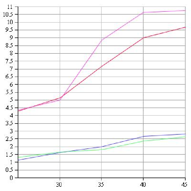
On the Fig. 1 I present the values of versus . Only the left, ascending part of the peak is plotted there, as it is less challenging for a manual computation. Unlike in [1], I used the estimator (4). The data points are binned into the groups of five, that is the values of the function are given only for values of the argument congruent to zero modulo five, and each ordinate is an average of five values, those from to . For even harmonics we see the peak, where the red line is the sample variance for all even coefficients, while the purple line is obtained with the estimator (4). The same is done for odd harmonics (the blue and the green lines), and a small valley is revealed. I won’t bet for the precise ordinates as I was calculating manually and rounding the data a little bit. But the general structure is represented correctly and agrees with the claim in the Ref. [1]. We can see that the peak is somewhat reduced compared to what was plotted in [1] without the separation of harmonics, at least in its relative weight, . And what is more important, the red line goes several times higher than the blue one. (And even the blue line is some factor of two higher than the actual primordial radiation [3].) This is true not only in average, but also for every single . It clearly shows that the dominant signal for these multipoles comes from the Galaxy, and it also heavily disproves the original hypothesis of having different observations of a one random variable. If is even, one also gets the large coefficients with large ’s more frequently than for the middle values of , as was stated in [1]. This effect is by far less pronounced than the difference between the red and the blue lines. But on the other hand, it shows that, even after the separation of different parity harmonics, the signal cannot be analysed reliably in this way. A considerable part of the initial peak came from the mixing of harmonics with essentially different levels of contamination which overweights the central part and the tails of the distribution. The remaining -even peak may also be the consequence of a non-uniform contamination, although the Galactic signal by itself is not very Gaussian. It could also be an interesting problem to compare the results of real and complex random variables analysis. The direction of zero Galactic longitude points at the Galactic center, and therefore cosine and sine harmonics might receive different contaminations.
The peak disappears when we go to larger and the spherical harmonics start probing the latitude scales smaller than the width of the bulk of Galactic signal. And therefore the different parity harmonics become not so different in the contamination level. For example, for estimated with -even harmonics is only few percent larger than estimated with -odd ones. (It is about .) Moreover, is quite large, and -even estimated without is a bit smaller than -odd.
It is hard to infer about the origin of the valley without knowing the detailed structure of the Galactic noise. It can come from some non-Gaussian properties of the noise. It can reflect some shortcomings of the foreground reduction procedures somehow oversubtracting the super-Gaussian noise from less affected coefficients. Probably, one could even devise a reasonable mixing of signals which would mimic a sub-Gaussian distribution, although it may require some bias of the mean values too.
5 Conclusions
In these notes I discussed the statistics behind the non-Gaussian anomalies reported in Ref. [1]. After that I have shown that the most probable explanation of the signal refers to geometric properties of the Galactic noise, and not to cosmology. Admittedly, I do not have a good understanding of the structure of Galactic noise. But at the very least, the claim for cosmological non-Gaussianities is pretty much premature. (I refer an interested reader to the work [1] for a different opinion.) On the other hand, one could probably use this kind of analysis to extract some information about the structure of the noise.
Acknowledgments. I am very grateful to the organizers of the Workshop for the opportunity to participate in this wonderful event, and especially I wish to thank Dominik Schwarz for invitation and for his encouragement to write this contribution. I am also very grateful to Pavel Naselsky and to other participants for very useful discussions. This work was supported in part by the Cluster of Excellence EXC 153 “Origin and Structure of the Universe”.
References
- [1] V. Vanchurin, Non-Gaussianity of the distribution tails in CMB, arXiv:0906.4954.
- [2] P. Naselsky, Discussion at the International Workshop on Cosmic Structure and Evolution.
- [3] G. Hinshaw et al., Five-Year Wilkinson Microwave Anisotropy Probe (WMAP) Observations: Data Processing, Sky Maps, and Basic Results, Astrophys.J.Suppl. 180 (2009) 225 [arXiv:0803.0732].