跳到论文正文
W Papers独立论文阅读器 arXiv:0910.5247 论文正文 计算阅读时间 · 0%
引用这篇论文根据当前论文元数据生成,正式投稿前建议核对。


License: arXiv.org perpetual non-exclusive license
arXiv:0910.5247v1 [math.AP] 28 Oct 2009

Global semigroup of conservative solutions of the nonlinear variational wave equationThanks: Supported in part by the Research Council of Norway. This paper was written as part of the international research program on Nonlinear Partial Differential Equations at the Centre for Advanced Study at the Norwegian Academy of Science and Letters in Oslo during the academic year 2008–09.

Helge Holden Holden
Department of Mathematical Sciences, Norwegian University of Science and Technology, NO–7491 Trondheim, Norway,
and
Centre of Mathematics for Applications, University of Oslo, P.O. Box 1053, Blindern, NO–0316 Oslo, Norway
Email address: holden@math.ntnu.no URL: www.math.ntnu.no/˜holden/
and Xavier Raynaud Raynaud
Centre of Mathematics for Applications, University of Oslo, P.O. Box 1053, Blindern, NO–0316 Oslo, Norway
Email address: raynaud@cma.uio.no
Date: August 24, 2026
Abstract.

We prove the existence of a global semigroup for conservative solutions of the nonlinear variational wave equation ut​t−c⁡(u)​(c⁡(u)​ux)x=0u_{tt}-c(u)(c(u)u_{x})_{x}=0. We allow for initial data u|t=0u|_{t=0} and ut|t=0u_{t}|_{t=0} that contain measures. We assume that 0<κ−1≤c⁡(u)≤κ0<\kappa^{-1}\leq c(u)\leq\kappa. Solutions of this equation may experience concentration of the energy density (ut2+c​(u)2​ux2)​d​x(u_{t}^{2}+c(u)^{2}u_{x}^{2})dx into sets of measure zero. The solution is constructed by introducing new variables related to the characteristics, whereby singularities in the energy density become manageable. Furthermore, we prove that the energy may only focus on a set of times of zero measure or at points where c′​(u)c^{\prime}(u) vanishes. A new numerical method to construct conservative solutions is provided and illustrated on examples.

Key words and phrases: 
Nonlinear variational wave equation, global semigroup, conservative solutions
2000 Mathematics Subject Classification
Primary: 35L70; Secondary: 49K20

1. Introduction

The nonlinear variational wave equation (NVW), which was first introduced by Saxton in [11], is given by the following nonlinear partial differential equation on the line

(1.1) ut​t−c⁡(u)​(c⁡(u)​ux)x=0u_{tt}-c(u)(c(u)u_{x})_{x}=0

with initial data

(1.2) u|t=0=u0,ut|t=0=u1.u|_{t=0}=u_{0},\ u_{t}|_{t=0}=u_{1}.

The equation can be derived from the variational principle applied to the functional

∬(ut2−c2​(u)​ux2)​𝑑x​𝑑t.\iint\left(u_{t}^{2}-c^{2}(u)u_{x}^{2}\right)\,dxdt.

We are interested in the analysis of conservative solutions of this initial value problem for u0,u1∈L2​(ℝ)u_{0},u_{1}\in L^{2}(\mathbb{R}). It is well known that solutions of this equation develop singularities in finite time, even for smooth initial data, see, e.g., [8]. The continuation past singularities is highly nontrivial, and allows for several distinct solutions. Thus additional information or requirements are needed to select a unique solution, and stability of solutions becomes a particularly delicate issue. We here study the conservative case where one in addition to the solution uu itself, requires that the energy is conserved. For smooth solutions the energy is given by ℰ⁡(t)=∫ℝ(ut2+c2​ux2)​(t,x)​𝑑x\mathcal{E}(t)=\int_{\mathbb{R}}(u_{t}^{2}+c^{2}u_{x}^{2})(t,x)\,dx. However, as energy may focus in isolated points, one has to look at energy density in the sense of measures such that the absolutely continuous part of the measure corresponds to the usual energy density. The analysis resembles to a large extent recent work done on the Camassa–Holm equation and the Hunter–Saxton equation (see, e.g., [9, 3, 13, 10] and references therein). Our main result is the proof of the existence of a global semigroup for conservative solutions of the NVW equation, allowing for concentration of the energy density on sets of zero measure.

The NVW equation has been extensively studied by Zhang and Zheng [12, 13, 14, 15, 16, 17, 18]. However, our approach is closely related to the approach by Bressan and Zheng [5], in that we introduce new variables based on the characteristics, thereby, loosely speaking, separating waves going in positive and negative direction.

It is difficult to illustrate the ideas in this paper as there are no elementary and explicit solutions available, except for the trivial case where cc is constant, which yields the classical linear wave equation. Thus one is forced to illustrate ideas numerically. Traditional finite difference schemes will not yield conservative solutions, but rather dissipative solutions due to the intrinsic numerical diffusion in these methods. Hence it is a challenge of separate interest to compute numerically conservative solutions of this equation to display some of the intricacies. This question is addressed and analyzed in Section 9.

Let us now turn to a more precise description of the content of this paper. We consider the variables RR and SS defined as

(1.3) {R=ut+c⁡(u)​ux,S=ut−c⁡(u)​ux.\left\{\begin{aligned} R&=u_{t}+c(u)u_{x},\\ S&=u_{t}-c(u)u_{x}.\end{aligned}\right.

By (1.1), we have

(1.4) {Rt−c​Rx=c′4​c​(R2−S2),St+c​Sx=c′4​c​(S2−R2),\left\{\begin{aligned} R_{t}-cR_{x}&=\frac{c^{\prime}}{4c}(R^{2}-S^{2}),\\ S_{t}+cS_{x}&=\frac{c^{\prime}}{4c}(S^{2}-R^{2}),\end{aligned}\right.

or, on conservative form,

(1.5) {(R2+S2)t−(c⁡(R2−S2))x=0,(1c​(R2−S2))t−(R2+S2)x=0.\left\{\begin{aligned} (R^{2}+S^{2})_{t}-(c(R^{2}-S^{2}))_{x}&=0,\\ (\frac{1}{c}(R^{2}-S^{2}))_{t}-(R^{2}+S^{2})_{x}&=0.\end{aligned}\right.

Let ℰ⁡(t)\mathcal{E}(t) denote the total energy of the system at time tt, i.e.,

(1.6) ℰ⁡(t)=∫ℝ(ut2+c2​ux2)​(t,x)​𝑑x=∫ℝ(R2+S2)​𝑑x.\mathcal{E}(t)=\int_{\mathbb{R}}(u_{t}^{2}+c^{2}u_{x}^{2})(t,x)\,dx=\int_{\mathbb{R}}(R^{2}+S^{2})\,dx.

We assume that the initial total energy that we denote ℰ0\mathcal{E}_{0} is finite and that uu is bounded in L∞L^{\infty}. For smooth solutions of (1.1) we have d​ℰd​t=0\frac{d\mathcal{E}}{dt}=0. We also assume that c∈C1​(ℝ)c\in C^{1}(\mathbb{R}) and c:ℝ→[κ−1,κ]c\colon\mathbb{R}\to[\kappa^{-1},\kappa] for some constant κ>0\kappa>0.

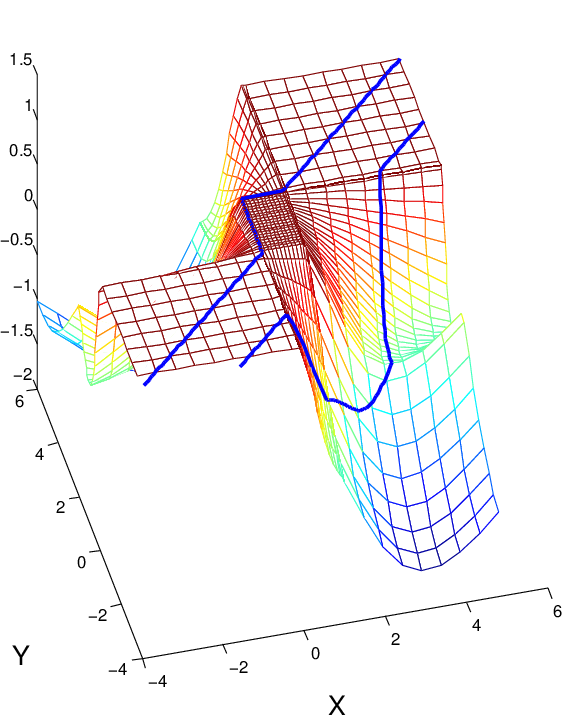
From (1.6) we see that we need that the functions RR and SS belong to L2​(ℝ)L^{2}(\mathbb{R}). It turns out that, as time evolves, the functions R2R^{2} and S2S^{2} can concentrate on sets of measure zero. The example presented in Figure 1, see Section 8.2, illustrates this phenomenon. In this case, we have a nontrivial solution uu for tt nonzero, which is however is identically equal to one at t=0t=0 and ut​(0,x)=0u_{t}(0,x)=0. However, when we analyze this example closer, we see that the energy concentrates at the origin, indeed

limt→0R2​(t,x)​d​x=δ and limt→0S2​(t,x)​d​x=2​δ\lim_{t\to 0}R^{2}(t,x)\,dx=\delta\quad\text{ and }\quad\lim_{t\to 0}S^{2}(t,x)\,dx=2\delta
Refer to caption
Refer to caption
Refer to caption
Figure 1. Plot of u⁡(t,x)u(t,x) for t=−3t=-3 (left), t=0t=0 (center), t=3t=3 (right).

where δ\delta is Dirac’s delta function. Clearly this complicates the existence and uniqueness question for this equation. As we want to construct a semigroup of solutions for this type of solutions, we have to know the location and amount of backward (R2R^{2}) and forward (S2S^{2}) energy that has concentrated on sets of zero measure, an information which is not given by the function uu itself. (In our example, since, at t=0t=0, the function uu is identically one and its time derivative utu_{t} identically zero, we cannot infer where the energy has concentrated.) Thus we introduce the set 𝒟\mathcal{D} whose elements, in addition to uu, RR, SS, contain two measures, μ\mu and ν\nu, corresponding to forward and backward energy density. More precisely, the measures are nonnegative Radon measures that satisfy

μac=14​R2​d​x,νac=14​S2​d​x.\mu_{\text{\rm ac}}=\frac{1}{4}R^{2}\,dx,\quad\nu_{\text{\rm ac}}=\frac{1}{4}S^{2}\,dx.

Our main contribution in this article is to present a rigorous construction of the semigroup of conservative solutions in 𝒟\mathcal{D}. Note that the set 𝒟\mathcal{D} is the natural set of solutions for conservative solutions, and the semigroup property can only be established in 𝒟\mathcal{D}, as illustrated by the example of Figure 1. Furthermore, by incorporating the energy measures as independent variables the formation of singularities is natural, and it allows for more general initial data. The present approach also provides a natural numerical method for conservative solutions.

As in [5], the construction of the solutions is achieved via a change of variables into a new coordinate system (X,Y)(X,Y) that straightens the characteristics. Even if we use different variables, the solutions we obtain are the same, but by extending the solutions to the set 𝒟\mathcal{D}, we are able to establish that the solutions we construct satisfy the semigroup property. We have to study in details the change of variables mapping — from the original variables to the new variables and vice versa — because, in order to prove the semigroup property, we have to establish that the two sets of variables match in an appropriate way. Compared to the variables used in [5], we prefer variables with a more direct physical interpretation. Namely, the variables we are considering are time, t⁡(X,Y)t(X,Y), space, x⁡(X,Y)x(X,Y), the solution function U⁡(X,Y)U(X,Y), which formally satisfies u⁡(t⁡(X,Y),x⁡(X,Y))=U⁡(X,Y)u(t(X,Y),x(X,Y))=U(X,Y) and the energy potentials JJ and KK. The definition of the energy potentials JJ and KK follows from (1.5), which says that the forms 14​(R2+S2)​d​x+14​c​(u)​(R2−S2)​d​t\frac{1}{4}(R^{2}+S^{2})\,dx+\frac{1}{4}c(u)(R^{2}-S^{2})\,dt and 14​c​(u)​(R2−S2)​d​x+14​(R2+S2)​d​t\frac{1}{4c(u)}(R^{2}-S^{2})\,dx+\frac{1}{4}(R^{2}+S^{2})dt are closed, so that, by Poincaré’s lemma, there exist functions, here denoted the energy potentials JJ and KK, whose differentials are equal to the given forms. Thus the new set of variables we will be considering equals Z=(t,x,U,J,K)Z=(t,x,U,J,K) and, after rewriting the governing equations (1.3) and (1.4) in the new coordinate system (X,Y)(X,Y), we get a system of equations of the form

(1.7) ZX​Y=F⁡(Z)​(ZX,ZY)Z_{XY}=F(Z)(Z_{X},Z_{Y})

where F⁡(Z):ℝ5×ℝ5→ℝ5F(Z)\colon\mathbb{R}^{5}\times\mathbb{R}^{5}\to\mathbb{R}^{5} is a bi-linear and symmetric operator, which depends only on UU, cf. (2.13).

In the new coordinates, the initial data corresponds to the set Γ0={(X,Y)∈ℝ2∣t⁡(X,Y)=0}\Gamma_{0}=\{(X,Y)\in\mathbb{R}^{2}\mid t(X,Y)=0\}. In the smooth case, Γ0\Gamma_{0} will be a strictly monotone curve. However, in our setting, Γ0\Gamma_{0} may not even be a curve, and even if it is a curve, it may not be continuous nor strictly monotone. Indeed, it may contain horizontal and vertical segments, and furthermore, rectangular boxes corresponding to the situation where both μ\mu and ν\nu are singular at the same point. If Γ0\Gamma_{0} is a curve with no vertical or horizontal parts and the initial data is bounded in L∞L^{\infty} (by initial data, we mean the values of ZZ, ZXZ_{X} and ZYZ_{Y} on Γ0\Gamma_{0}), then the existence and uniqueness of solutions to (1.7) is a classical result, see, for example, [7, Ch. 4]. In the present paper we have to deal with unbounded data in 𝒟\mathcal{D} (uxu_{x} and utu_{t} are unbounded in L∞L^{\infty}). The new coordinates (X,Y)(X,Y) are given by

d​x−c⁡(u)​d​t=0​ if and only if ​d​Y=0dx-c(u)dt=0\text{ if and only if }dY=0

and

d​x+c⁡(u)​d​t=0​ if and only if ​d​X=0,dx+c(u)dt=0\text{ if and only if }dX=0,

that is, the characteristics are mapped to horizontal and vertical lines. We denote by 𝐋\mathbf{L} the mapping from the possible initial data in 𝒟\mathcal{D} to the set ℱ\mathcal{F} defined by Γ0\Gamma_{0} and the value of the initial data on Γ0\Gamma_{0}, thus 𝐋:𝒟→ℱ\mathbf{L}\colon\mathcal{D}\to\mathcal{F}, see Definition 3.8. From Γ0\Gamma_{0} we have to select one curve that can be used as initial data for the equation (1.7). There is a certain nonuniqueness due to fact that Γ0\Gamma_{0} may not be curve. Let 𝒢0\mathcal{G}_{0} denote the set of all curves, including the information about the initial data. We let 𝐂\mathbf{C} denote the mapping that from a set Γ0\Gamma_{0} selects one possible curve, that is, 𝐂:ℱ→𝒢0\mathbf{C}\colon\mathcal{F}\to\mathcal{G}_{0}, see Definition 3.5. The inverse map that from curve determines the corresponding set in ℱ\mathcal{F} is denoted 𝐃\mathbf{D}, see Definition 3.7. Once we have a curve with the initial data, we can in principle compute the solution by solving (1.7). To show the existence of a global solution we use the the bi-linearity of (1.7) and an a priori bound on the energy potentials JJ and KK, see Section 4. We let the set of all possible solutions be denoted by ℋ\mathcal{H}, and let 𝐒:𝒢→ℋ\mathbf{S}\colon\mathcal{G}\to\mathcal{H} denote the map that computes the solution that passes through the curve in 𝒢\mathcal{G}, see Theorem 4.15. Here 𝒢\mathcal{G} is defined as 𝒢0\mathcal{G}_{0} without the constraint that t=0t=0, see Definition 3.2. Recall that as tt now is a dependent variable, it does not make sense to compute the solution up to a specific time, but rather we determine the global solution for all times. Thus we need a mapping that extracts the solution ZZ for a given time TT, that is, the intersection of the solution in ℋ\mathcal{H} with the set where t⁡(X,Y)=Tt(X,Y)=T. Let 𝐄:ℋ→𝒢0\mathbf{E}\colon\mathcal{H}\to\mathcal{G}_{0} denote the map that from any given solution in ℋ\mathcal{H} extracts the solution at t=0t=0, that is, in 𝒢0\mathcal{G}_{0}, see Definition 5.1. Next we define the operator 𝐭T:ℋ→ℋ\mathbf{t}_{T}\colon\mathcal{H}\to\mathcal{H} that shifts time in a solution in ℋ\mathcal{H} by a given time TT, see Definition 5.2. Now we can define the map ST:ℱ→ℱS_{T}\colon\mathcal{F}\to\mathcal{F} by ST=𝐃∘𝐄∘𝐭T∘𝐒∘𝐂S_{T}=\mathbf{D}\circ\mathbf{E}\circ\mathbf{t}_{T}\circ\mathbf{S}\circ\mathbf{C}, see Definition 5.4. A key result is that STS_{T} is a semigroup on ℱ\mathcal{F}, see Theorem 5.5. Next we need to return to the original variables. Let 𝐌:ℱ→𝒟\mathbf{M}\colon\mathcal{F}\to\mathcal{D} denote that map, see Definition 6.1. Thus the solution operator S¯T:𝒟→𝒟\bar{S}_{T}\colon\mathcal{D}\to\mathcal{D} is defined by (Definition 6.4)

(1.8) S¯T=𝐌∘ST∘𝐋.\bar{S}_{T}=\mathbf{M}\circ S_{T}\circ\mathbf{L}.

It remains to show that S¯T\bar{S}_{T} is a semigroup. However, since 𝐌\mathbf{M} is not inverse of 𝐋\mathbf{L}, as 𝐋∘𝐌≠Idℱ\mathbf{L}\circ\mathbf{M}\neq\id_{\mathcal{F}}, the semigroup property of S¯T\bar{S}_{T} still does not follow from (1.8). This fact is explained as follows. When changing variables, we have introduced a degree of freedom that we now want to eliminate. This degree of freedom can be identified precisely with the action of the group G2G^{2}, where GG denotes the group of diffeomorphisms of the real line. Indeed, by simply using the bi-linearity of (1.7), one can check that if ZZ is a solution to (1.7), then Z¯​(X,Y)=Z⁡(f⁡(X),g⁡(Y))\bar{Z}(X,Y)=Z(f(X),g(Y)), where (f,g)∈G2(f,g)\in G^{2}, is also a solution to the same equation. The transformation (X,Y)↦(f⁡(X),g⁡(Y))(X,Y)\mapsto(f(X),g(Y)) corresponds to a stretching of the plane ℝ2\mathbb{R}^{2} in the XX and YY directions. Note that this transformation maps horizontal (resp. vertical) lines to horizontal (resp. vertical) lines and therefore preserves the directions of the characteristics. Moreover, this transformation does not affect the solution in the original coordinates. To illustrate this we ignore for the moment for the sake of simplicity, the energies μ\mu and ν\nu in the definition of 𝒟\mathcal{D}. The solution u⁡(t,x)u(t,x) can be seen as the surface in ℝ3\mathbb{R}^{3} given by (t,x,u⁡(t,x))(t,x,u(t,x)) where (t,x)∈ℝ2(t,x)\in\mathbb{R}^{2} are parameters. Through our change of variables, we obtain another parametrization of the same surface, namely,

(1.9) (t⁡(X,Y),x⁡(X,Y),U⁡(X,Y))(t(X,Y),x(X,Y),U(X,Y))

where (X,Y)∈ℝ2(X,Y)\in\mathbb{R}^{2} are the new parameters. Additional properties of the solution Z=(t,x,U,J,K)Z=(t,x,U,J,K) which are contained in the definition of ℋ\mathcal{H} guarantee that the surface defined by (1.9) does not fold over itself so that it is in fact a graph. It is then clear from (1.9) that the transformation (X,Y)↦(f⁡(X),g⁡(Y))(X,Y)\mapsto(f(X),g(Y)) is simply a re-parametrization of the same surface, which defines u⁡(t,x)u(t,x) uniquely. At the level of the set ℱ\mathcal{F}, which corresponds to a parametrization of the initial data in the new coordinates, we can also define the action of the group G2G^{2} that denote ψ×(f,g)↦ψ⋅(f,g)\psi\times(f,g)\mapsto\psi\cdot(f,g) for any ψ∈ℱ\psi\in\mathcal{F} and (f,g)∈G2(f,g)\in G^{2}. We prove that two elements which are equivalent correspond to the same element in 𝒟\mathcal{D}, that is,

(1.10) 𝐌⁡(ψ¯)=𝐌⁡(ψ)\mathbf{M}(\bar{\psi})=\mathbf{M}(\psi)

where ψ¯=ψ⋅(f,g)\bar{\psi}=\psi\cdot(f,g) for some (f,g)∈G2(f,g)\in G^{2}. From (1.10), it is now clear why 𝐋∘𝐌≠Idℱ\mathbf{L}\circ\mathbf{M}\neq\id_{\mathcal{F}} as, in general, ψ¯\bar{\psi} and ψ\psi are distinct. We introduce a subset ℱ0\mathcal{F}_{0} of ℱ\mathcal{F} which corresponds to a section of ℱ\mathcal{F} with respect to the action of the group G2G^{2}, which means that the set ℱ0\mathcal{F}_{0} contains only one representative of each equivalence class so that ℱ/G2\mathcal{F}/G^{2} and ℱ0\mathcal{F}_{0} are in bijection. The system (1.7) preserves the strict positivity of the quantities xX+JXx_{X}+J_{X} and xY+JYx_{Y}+J_{Y} and the set ℱ\mathcal{F} somehow inherits this property which makes it possible to define the projection Π:ℱ→ℱ0\Pi\colon\mathcal{F}\to\mathcal{F}_{0}. The projection Π\Pi associates to any element in ℱ\mathcal{F} its unique representative in ℱ0\mathcal{F}_{0} which belongs to the same equivalence class. As expected, since we have now eliminated the degree of freedom we introduced by changing variables, we obtain that ℱ0\mathcal{F}_{0} and 𝒟\mathcal{D} are in bijection. We are then able to prove that S¯t\bar{S}_{t} is a semigroup.

Our main result, Theorem 7.9, reads as follows:
Theorem. Given (u0,R0,S0,μ0,ν0)∈𝒟(u_{0},R_{0},S_{0},\mu_{0},\nu_{0})\in\mathcal{D}, let us denote (u,R,S,μ,ν)​(t)=S¯t​(u0,R0,S0,μ0,ν0)(u,R,S,\mu,\nu)(t)=\bar{S}_{t}(u_{0},R_{0},S_{0},\mu_{0},\nu_{0}). Then uu is a weak solution of the nonlinear variational wave equation (1.1), that is,

(1.11) ∫ℝ2(ϕt−(c⁡(u)​ϕ)x)​R​𝑑x​𝑑t+∫ℝ2(ϕt+(c⁡(u)​ϕ)x)​S​𝑑x​𝑑t=0\int_{\mathbb{R}^{2}}(\phi_{t}-(c(u)\phi)_{x})R\,dxdt+\int_{\mathbb{R}^{2}}(\phi_{t}+(c(u)\phi)_{x})S\,dxdt=0

for all smooth functions ϕ\phi with compact support and where

(1.12) R=ut+c⁡(u)​ux,S=ut−c⁡(u)​ux.R=u_{t}+c(u)u_{x},\quad S=u_{t}-c(u)u_{x}.

Moreover, the measures μ⁡(t)\mu(t) and ν⁡(t)\nu(t) satisfy the following equations in the sense of distribution

(1.13a) (μ+ν)t−(c⁡(μ−ν))x=0(\mu+\nu)_{t}-(c(\mu-\nu))_{x}=0
and
(1.13b) (1c​(μ−ν))t−(μ+ν)x=0.(\frac{1}{c}(\mu-\nu))_{t}-(\mu+\nu)_{x}=0.

The mapping S¯T:𝒟→𝒟\bar{S}_{T}:\mathcal{D}\to\mathcal{D} is a semigroup, that is,

S¯t+t′=S¯t∘S¯t′\bar{S}_{t+t^{\prime}}=\bar{S}_{t}\circ\bar{S}_{t^{\prime}}

for all positive tt and t′t^{\prime}.

Furthermore, we note the following important result (Theorem 7.10):
Theorem. The solution satisfies the following properties:

  1. (i)

    For all t∈ℝt\in\mathbb{R}

    (1.14) μ⁡(t)​(ℝ)+ν⁡(t)​(ℝ)=μ0​(ℝ)+ν0​(ℝ).\mu(t)(\mathbb{R})+\nu(t)(\mathbb{R})=\mu_{0}(\mathbb{R})+\nu_{0}(\mathbb{R}).
  2. (ii)

    For almost every t∈ℝt\in\mathbb{R}, the singular part of μ⁡(t)\mu(t) and ν⁡(t)\nu(t) are concentrated on the set where c′​(u)=0c^{\prime}(u)=0.

In this article, we do not study the stability of the solutions. However, since the solutions we obtain coincide with the ones obtained in [5] for initial data which do not contain any singular measure, the solutions in that case also satisfy the stability result stated in [5, Theorem 2]. To obtain a continuous semigroup of solution in 𝒟\mathcal{D}, we would like to follow the approach developed in [9], [4] for the Camassa–Holm equation and Hunter–Saxton equations. In these two papers, the conservative solutions are also obtained via a change of variables which is invariant with respect to relabeling (i.e., with respect to the action of the group of diffeomorphisms GG). We define a distance between equivalence classes in the new coordinates. This distance is then mapped back to the original set of coordinates so that we obtain a continuous semigroup for this metric. In the case of the nonlinear wave equation, in particular, because of the truly two dimensional nature of the problem, it is not so easy to formulate a stability result in the new coordinates which holds when mapping back to the original set of variables. In Lemma 4.12 we present a result in that direction.

There is a lack of explicit solutions to NVW. In this paper we consider two explicit examples. The first example, see Section 8.1, is the simplest possible, namely the linear wave equation (with cc constant), but with general initial data. We recover as expected the familiar d’Alembert solution. The energy measures are transported with velocity ±c\pm c. The second example, see Section 8.2, is a truly nonlinear case with velocity given by (1.19). However, here we choose the simplest nontrivial initial data with energy concentration initially for both measures. The corresponding equation (1.7) is solved numerically, and the result is illustrated on Figs. 1, 9–12.

The numerical method that yields conservative solutions is described in Section 9.

1.1. Physical motivation for the nonlinear variational wave equation

The NVW equation was first derived in the context of nematic liquid crystals, see [11, 10]. More precisely, a nematic crystal can be described, when we ignore the motion of the fluid, by the dynamics of the so-called director field 𝐧=𝐧⁡(x,y,z,t)∈ℝ3\mathbf{n}=\mathbf{n}(x,y,z,t)\in\mathbb{R}^{3} describing the orientation of rod-like molecules. Thus |𝐧|=1\left|\mathbf{n}\right|=1. The Oseen–Franck strain-energy potential is given by

(1.15) W(𝐧,∇𝐧)=α|𝐧×(∇×𝐧)|2+β(∇⋅𝐧)2+γ(𝐧⋅∇×𝐧)2,W(\mathbf{n},\nabla\mathbf{n})=\alpha\left|\mathbf{n}\times(\nabla\times\mathbf{n})\right|^{2}+\beta(\nabla\cdot\mathbf{n})^{2}+\gamma(\mathbf{n}\cdot\nabla\times\mathbf{n})^{2},

where α,β,γ\alpha,\beta,\gamma are constitutive constants. Consider next the highly simplified case of director fields of the type

(1.16) 𝐧=𝐧⁡(x,t)=cos⁡(u⁡(t,x))​𝐞x+sin⁡(u⁡(t,x))​𝐞y\mathbf{n}=\mathbf{n}(x,t)=\cos(u(t,x))\mathbf{e}_{x}+\sin(u(t,x))\mathbf{e}_{y}

where 𝐞x\mathbf{e}_{x} and 𝐞y\mathbf{e}_{y} are unit vectors in the xx and yy direction, respectively. In this case the functional W⁡(𝐧,∇𝐧)W(\mathbf{n},\nabla\mathbf{n}) vastly simplifies to

(1.17) W⁡(𝐧,∇𝐧)=(β​cos2⁡u+α​sin2⁡u)​ux2,W(\mathbf{n},\nabla\mathbf{n})=(\beta\cos^{2}u+\alpha\sin^{2}u)u_{x}^{2},

and |𝐧t|2=ut2\left|\mathbf{n}_{t}\right|^{2}=u_{t}^{2}. The dynamics is described by the variational principle

(1.18) δδ​u​∬(ut2−c2​(u)​ux2)​𝑑x​𝑑t=0,\frac{\delta}{\delta u}\iint\big(u_{t}^{2}-c^{2}(u)u_{x}^{2}\big)dxdt=0,

where

(1.19) c2​(u)=β​cos2⁡u+α​sin2⁡u,c^{2}(u)=\beta\cos^{2}u+\alpha\sin^{2}u,

which results in the nonlinear variational wave equation

(1.20) ut​t−c⁡(u)​(c⁡(u)​ux)x=0.u_{tt}-c(u)(c(u)u_{x})_{x}=0.

2. Equivalent system for the NVW equation

In this section, we assume the existence of a smooth solution u=u⁡(t,x)u=u(t,x) to (1.1). We introduce the change of variables (t,x)↦(X,Y)(t,x)\mapsto(X,Y) which straightens out the characteristics: The forward characteristics, which are given by the solutions of d​xd​t=c⁡(u⁡(t,x⁡(t)))\frac{dx}{dt}=c(u(t,x(t))), are mapped to the horizontal lines while the backward characteristics, which are given by the solutions of d​xd​t=−c⁡(u⁡(t,x⁡(t)))\frac{dx}{dt}=-c(u(t,x(t))), are mapped to the vertical lines. Formally, we can rewrite these conditions as

(2.1) d​x−c⁡(u)​d​t=0​ if and only if ​d​Y=0dx-c(u)dt=0\text{ if and only if }dY=0

and

(2.2) d​x+c⁡(u)​d​t=0​ if and only if ​d​X=0.dx+c(u)dt=0\text{ if and only if }dX=0.

Our goal now is to rewrite the governing equation (1.1) in terms of the new variables (X,Y)(X,Y). The variables (t,x)(t,x) become functions of (X,Y)(X,Y) that we denote t⁡(X,Y)t(X,Y) and x⁡(X,Y)x(X,Y). We set

(2.3) U⁡(X,Y)=u⁡(t,x).U(X,Y)=u(t,x).

Since

d​x=xX​d​X+xY​d​Y​ and ​d​t=tX​d​X+tY​d​Y,dx=x_{X}dX+x_{Y}dY\ \text{ and }\ dt=t_{X}dX+t_{Y}dY,

we obtain from (2.1) and (2.2) that

(2.4) xX=c⁡(U)​tX​ and ​xY=−c⁡(U)​tY.x_{X}=c(U)t_{X}\ \text{ and }\ x_{Y}=-c(U)t_{Y}.

From (1.5), we infer that the forms 14​(R2+S2)​d​x+c4​(R2−S2)​d​t\frac{1}{4}(R^{2}+S^{2})dx+\frac{c}{4}(R^{2}-S^{2})dt and 14​c​(R2−S2)​d​x+14​(R2+S2)​d​t\frac{1}{4c}(R^{2}-S^{2})dx+\frac{1}{4}(R^{2}+S^{2})dt are closed. Therefore, by Poincaré’s lemma, we infer the existence of two functions JJ and KK for which these forms are the differentials, that is,

(2.5) d​J=14​(R2+S2)​d​x+c4​(R2−S2)​d​tdJ=\frac{1}{4}(R^{2}+S^{2})dx+\frac{c}{4}(R^{2}-S^{2})dt

and

(2.6) d​K=14​c​(R2−S2)​d​x+14​(R2+S2)​d​t.dK=\frac{1}{4c}(R^{2}-S^{2})dx+\frac{1}{4}(R^{2}+S^{2})dt.

We have, after using (2.4),

d​J\displaystyle dJ =14​(R2+S2)​d​x+c4​(R2−S2)​d​t\displaystyle=\frac{1}{4}(R^{2}+S^{2})dx+\frac{c}{4}(R^{2}-S^{2})dt
=14​(R2+S2)​(xX​d​X+xY​d​Y)+c4​(R2−S2)​(tX​d​X+tY​d​Y)\displaystyle=\frac{1}{4}(R^{2}+S^{2})(x_{X}dX+x_{Y}dY)+\frac{c}{4}(R^{2}-S^{2})(t_{X}dX+t_{Y}dY)
=12​R2​xX​d​X+12​S2​xY​d​Y,\displaystyle=\frac{1}{2}R^{2}x_{X}dX+\frac{1}{2}S^{2}x_{Y}dY,

and, similarly, we get

d​K=R22​c​xX​d​X−S22​c​xY​d​YdK=\frac{R^{2}}{2c}x_{X}dX-\frac{S^{2}}{2c}x_{Y}dY

so that

(2.7) JX=c⁡(U)​KX​ and ​JY=−c⁡(U)​KYJ_{X}=c(U)K_{X}\ \text{ and }\ J_{Y}=-c(U)K_{Y}

hold. Note the similarity between the relations (2.7) for the pair (J,K)(J,K) and the relations (2.4) for the pair (t,x)(t,x). We want to compute the mixed second derivatives of our new variables, namely, tt, xx, UU, JJ and KK. By (2.4), we obtain

d​t=tX​d​X+tY​d​Y=1c​xX​d​X−1c​xY​d​Y.dt=t_{X}dX+t_{Y}dY=\frac{1}{c}x_{X}dX-\frac{1}{c}x_{Y}dY.

By expressing the fact that the form d​tdt is closed (since it is exact), we get

∂∂Y​(1c​xX)=−∂∂X​(1c​xY)\frac{\partial}{\partial Y}\left(\frac{1}{c}x_{X}\right)=-\frac{\partial}{\partial X}\left(\frac{1}{c}x_{Y}\right)

which implies

xX​Y=c′2​c​(uY​xX+uX​xY).{x}_{XY}=\frac{c^{\prime}}{2c}\left(u_{Y}x_{X}+u_{X}x_{Y}\right).

Similarly, since the form

d​x=xX​d​X+xY​d​Y=c​tX​d​X−c​tY​d​Ydx=x_{X}dX+x_{Y}dY=ct_{X}dX-ct_{Y}dY

is closed, we obtain

∂∂Y​(c​tX)=−∂∂X​(c​tY)\frac{\partial}{\partial Y}\left(ct_{X}\right)=-\frac{\partial}{\partial X}\left(ct_{Y}\right)

which implies

tX​Y=−c′2​c​(uX​tY+uY​tX).{t}_{XY}=-\frac{c^{\prime}}{2c}\left(u_{X}t_{Y}+u_{Y}t_{X}\right).

By using the relations (2.7), the form d​KdK can be rewritten as

d​K=1c​JX​d​X−1c​JY​d​YdK=\frac{1}{c}J_{X}dX-\frac{1}{c}J_{Y}dY

and, expressing the fact that d​KdK is a closed, we obtain

∂∂Y​(1c​JX)=∂∂X​(−1c​JY)\frac{\partial}{\partial Y}\left(\frac{1}{c}J_{X}\right)=\frac{\partial}{\partial X}\left(-\frac{1}{c}J_{Y}\right)

which yields

JX​Y=c′2​c​(JX​UY+JY​UX).{J}_{XY}=\frac{c^{\prime}}{2c}\left(J_{X}U_{Y}+J_{Y}U_{X}\right).

Similarly, we can rewrite the form d​JdJ as

d​K=c​KX​d​X−c​KY​d​YdK=cK_{X}dX-cK_{Y}dY

and, expressing the fact d​KdK is closed, we get

KX​Y=−c′2​c​(KX​UY+KY​UX).{K}_{XY}=-\frac{c^{\prime}}{2c}\left(K_{X}U_{Y}+K_{Y}U_{X}\right).

Let us consider the forms

(2.8) ω1=R2​c​d​x+12​R​d​t\omega_{1}=\frac{R}{2c}dx+\frac{1}{2}Rdt

and

(2.9) ω2=S2​c​d​x−12​S​d​t.\omega_{2}=\frac{S}{2c}dx-\frac{1}{2}Sdt.

In the new variables, these forms rewrite

ω1\displaystyle\omega_{1} =ut+c​ux2​c​(xX​d​X+xY​d​Y)+12​(ut+c​ux)​(tX​d​X+tY​d​Y)\displaystyle=\frac{u_{t}+cu_{x}}{2c}(x_{X}dX+x_{Y}dY)+\frac{1}{2}(u_{t}+cu_{x})(t_{X}dX+t_{Y}dY)
=(uttX+uxxX)dX (after using (2.4))\displaystyle=(u_{t}t_{X}+u_{x}x_{X})dX\quad\text{ (after using \eqref{eq:chardef})}
(2.10) =UX​d​X,\displaystyle=U_{X}dX,

and, similarly, we find

(2.11) ω2=−UY​d​Y.\omega_{2}=-U_{Y}dY.

From (2.8), by using (1.4), we obtain

d​ω1\displaystyle d\omega_{1} =(Rt2​c−c′​R2​c2​ut)​d​t∧d​x+12​Rx​d​x∧d​t\displaystyle=(\frac{R_{t}}{2c}-\frac{c^{\prime}R}{2c^{2}}u_{t})dt\wedge dx+\frac{1}{2}R_{x}dx\wedge dt
=Rt−c​Rx2​c​d​t∧d​x−c′​R2​c2​12​(R+S)​d​t∧d​x\displaystyle=\frac{R_{t}-cR_{x}}{2c}dt\wedge dx-\frac{c^{\prime}R}{2c^{2}}\frac{1}{2}(R+S)dt\wedge dx
=(c′​(R2−S2)8​c2−c′​R2​c2​12​(R+S))​d​t∧d​x\displaystyle=\Big(\frac{c^{\prime}(R^{2}-S^{2})}{8c^{2}}-\frac{c^{\prime}R}{2c^{2}}\frac{1}{2}(R+S)\Big)\,dt\wedge dx
=c′2​c2​(12​(R+S))2​d​x∧d​t=c′2​c2​ut2​d​x∧d​t,\displaystyle=\frac{c^{\prime}}{2c^{2}}\left(\frac{1}{2}(R+S)\right)^{2}dx\wedge dt=\frac{c^{\prime}}{2c^{2}}u_{t}^{2}dx\wedge dt,

and, furthermore, we obtain

d​ω1\displaystyle d\omega_{1} =c′2​c2​(14​(R2+S2)​d​x∧d​t+12​R​S​d​x∧d​t)\displaystyle=\frac{c^{\prime}}{2c^{2}}\Big(\frac{1}{4}(R^{2}+S^{2})dx\wedge dt+\frac{1}{2}RSdx\wedge dt\Big)
(2.12) =c′2​c2​d​J∧d​t−c′2​c​ω1∧ω2\displaystyle=\frac{c^{\prime}}{2c^{2}}dJ\wedge dt-\frac{c^{\prime}}{2c}\omega_{1}\wedge\omega_{2}

because

ω1∧ω2=−R​S2​c​d​x∧d​t.\displaystyle\omega_{1}\wedge\omega_{2}=-\frac{RS}{2c}dx\wedge dt.

We rewrite (2.12) in the new set of variables

d​ω1\displaystyle d\omega_{1} =c′2​c2​(JX​d​X+JY​d​Y)∧(tX​d​X+tY​d​Y)−c′2​c​ω1∧ω2\displaystyle=\frac{c^{\prime}}{2c^{2}}(J_{X}dX+J_{Y}dY)\wedge(t_{X}dX+t_{Y}dY)-\frac{c^{\prime}}{2c}\omega_{1}\wedge\omega_{2}
=−c′2​c3​(JX​xY+JY​xX)​d​X∧d​Y+c′2​c​UX​UY​d​X∧d​Y.\displaystyle=-\frac{c^{\prime}}{2c^{3}}(J_{X}x_{Y}+J_{Y}x_{X})dX\wedge dY+\frac{c^{\prime}}{2c}U_{X}U_{Y}dX\wedge dY.

At the same time, by (2.10), we have d​ω1=−UX​Y​d​X∧d​Yd\omega_{1}=-{U}_{XY}dX\wedge dY, and therefore it follows that

UX​Y=c′2​c3​(JX​xX+JY​xX)−c′2​c​UX​UY.{U}_{XY}=\frac{c^{\prime}}{2c^{3}}\left(J_{X}x_{X}+J_{Y}x_{X}\right)-\frac{c^{\prime}}{2c}U_{X}U_{Y}.

Finally, we obtain following system of equations

(2.13a) tX​Y\displaystyle{t}_{XY} =−c′2​c​(UX​tY+UY​tX),\displaystyle=-\frac{c^{\prime}}{2c}\left(U_{X}t_{Y}+U_{Y}t_{X}\right),
(2.13b) xX​Y\displaystyle{x}_{XY} =c′2​c​(UY​xX+UX​xY),\displaystyle=\frac{c^{\prime}}{2c}\left(U_{Y}x_{X}+U_{X}x_{Y}\right),
(2.13c) UX​Y\displaystyle{U}_{XY} =c′2​c3​(xY​JX+JY​xX)−c′2​c​UY​UX,\displaystyle=\frac{c^{\prime}}{2c^{3}}\left(x_{Y}J_{X}+J_{Y}x_{X}\right)-\frac{c^{\prime}}{2c}U_{Y}U_{X},
(2.13d) JX​Y\displaystyle{J}_{XY} =c′2​c​(JX​UY+JY​UX),\displaystyle=\frac{c^{\prime}}{2c}\left(J_{X}U_{Y}+J_{Y}U_{X}\right),
(2.13e) KX​Y\displaystyle{K}_{XY} =−c′2​c​(KX​UY+KY​UX).\displaystyle=-\frac{c^{\prime}}{2c}\left(K_{X}U_{Y}+K_{Y}U_{X}\right).

Let ZZ denote the vector (t,x,U,J,K)(t,x,U,J,K). The system (2.13) then rewrites as

(2.14) ZX​Y=F⁡(Z)​(ZX,ZY)Z_{XY}=F(Z)(Z_{X},Z_{Y})

where F⁡(Z)F(Z) is a bi-linear and symmetric tensor from ℝ5×ℝ5\mathbb{R}^{5}\times\mathbb{R}^{5} to ℝ5\mathbb{R}^{5}. Due to the relations (2.4), either one of the equations (2.13a) and (2.13b) is redundant: one could remove one of them, and the system would remain well-posed, and one retrieves tt or xx by using (2.4). Similarly, either one of the equations (2.13d) and (2.13e) becomes redundant by (2.7). However, we find it convenient to work with the complete set of variables, that is, Z=(t,x,U,J,K)Z=(t,x,U,J,K). We will see later that the solutions of the system (2.13) preserve these conditions.

To prove the existence of solutions to (2.13), we use a fixed point argument. The argument is similar to the one that can be found for example in [7] and in [5]. However, in order to take into account the non-regularity of the data (u0​xu_{0x} and u0​tu_{0t} are in L2L^{2} and the energy can concentrate on sets of zero measure), we have to consider, in the new set of coordinates, data given on curves which have parts which are parallel to the characteristic directions. In particular, the curves are not given as graphs of a function. We are looking for a solution that satisfies a given initial condition at time t=0t=0. In the (X,Y)(X,Y) plane, the set of points which correspond to initial time, that is, t⁡(X,Y)=0t(X,Y)=0, may be a curve, (𝒳⁡(s),𝒴⁡(s))∈ℝ2(\mathcal{X}(s),\mathcal{Y}(s))\in\mathbb{R}^{2}, parametrized by s∈ℝs\in\mathbb{R}, but it may also be a more complicated set, see Figure 2 that we will comment on later. We consider curves of the following type.

Definition 2.1.

We denote by 𝒞\mathcal{C} the set of curves in the plane ℝ2\mathbb{R}^{2} parametrized by (𝒳⁡(s),𝒴⁡(s))(\mathcal{X}(s),\mathcal{Y}(s)) with s∈ℝs\in\mathbb{R}, such that

(2.15a) 𝒳−Id,𝒴−Id∈W1,∞​(ℝ),\displaystyle\mathcal{X}-\id,\ \mathcal{Y}-\id\in W^{1,\infty}(\mathbb{R}),
(2.15b) ˙​𝒳≥0,˙​𝒴≥0\displaystyle\dot{}\mathcal{X}\geq 0,\quad\dot{}\mathcal{Y}\geq 0
and the normalization
(2.15c) 12(𝒳(s)+𝒴(s))=s, for all s∈ℝ.\frac{1}{2}(\mathcal{X}(s)+\mathcal{Y}(s))=s,\text{ for all }s\in\mathbb{R}.

We set

(2.16) ‖(𝒳,𝒴)‖𝒞=‖𝒳−Id‖L∞+‖𝒳−Id‖L∞.\left\|(\mathcal{X},\mathcal{Y})\right\|_{\mathcal{C}}=\left\|\mathcal{X}-\id\right\|_{L^{\infty}}+\left\|\mathcal{X}-\id\right\|_{L^{\infty}}.

From the initial data (u0,R0,S0)(u_{0},R_{0},S_{0}), we want to define the curve Γ0=(𝒳⁡(s),𝒴⁡(s))\Gamma_{0}=(\mathcal{X}(s),\mathcal{Y}(s)) in 𝒞\mathcal{C} which corresponds to the initial time and the value of ZZ on this curve. To solve the governing equations (2.13), we need to know the values of ZZ, ZXZ_{X} and ZYZ_{Y} on the curve Γ0\Gamma_{0}. In total, we have to determine 17 unknown functions. Given the initial data (u0,R0,S0)(u_{0},R_{0},S_{0}), there is no unique way to define the curve (𝒳⁡(s),𝒴⁡(s))(\mathcal{X}(s),\mathcal{Y}(s)) and the values of ZZ on this curve in order to obtain to the desired solution. This fact is due to the relabeling symmetry, a degree of freedom which is embedded in the set of equations (2.13) that we precisely identify in Section 7. For now, the goal is to use this degree of freedom to construct an initial data which is bounded in L∞​(ℝ)L^{\infty}(\mathbb{R}) on the curve. Let us now explain how we proceed for an initial data (u0,R0,S0)∈[L2​(ℝ)]3(u_{0},R_{0},S_{0})\in[L^{2}(\mathbb{R})]^{3} for which energy has not concentrated and we will see later how to extend this construction to initial data containing singular measures. In this case, the function 𝒳\mathcal{X} and 𝒴\mathcal{Y} are invertible and, slightly abusing notation, we denote by Z⁡(s)Z(s), ZX​(X)Z_{X}(X) and ZY​(Y)Z_{Y}(Y) the values of Z⁡(𝒳⁡(s),𝒴⁡(s))Z(\mathcal{X}(s),\mathcal{Y}(s)), ZX​(X,𝒴⁡(𝒳−1​(X)))Z_{X}(X,\mathcal{Y}(\mathcal{X}^{-1}(X))) and ZY​(𝒳⁡(𝒴−1​(Y)),Y)Z_{Y}(\mathcal{X}(\mathcal{Y}^{-1}(Y)),Y), respectively. By definition, we have

(2.17) t⁡(s)=0,t(s)=0,

and, naturally, we set

(2.18) U⁡(s)=u0​(x⁡(s)).U(s)=u_{0}(x(s)).

From the formal derivation of the previous section, we have the following relations

(2.19) JX​(𝒳)\displaystyle J_{X}(\mathcal{X}) =c⁡(u)​KX​(𝒳)=12​R02​(x)​xX​(𝒳),\displaystyle=c(u)K_{X}(\mathcal{X})=\frac{1}{2}R_{0}^{2}(x)x_{X}(\mathcal{X}), JY​(𝒴)\displaystyle J_{Y}(\mathcal{Y}) =−c⁡(u)​KY​(𝒴)=12​S02​(x)​xY​(𝒴),\displaystyle=-c(u)K_{Y}(\mathcal{Y})=\frac{1}{2}S_{0}^{2}(x)x_{Y}(\mathcal{Y}),
(2.20) UX​(𝒳)\displaystyle U_{X}(\mathcal{X}) =R0​(x)c⁡(u⁡(x))​xX​(𝒳),\displaystyle=\frac{R_{0}(x)}{c(u(x))}x_{X}(\mathcal{X}), UY​(𝒴)\displaystyle U_{Y}(\mathcal{Y}) =−S0​(x)c⁡(u⁡(x))​xY​(𝒴).\displaystyle=-\frac{S_{0}(x)}{c(u(x))}x_{Y}(\mathcal{Y}).

We have the compatibility condition

(2.21) Z˙​(s)=ZX​(𝒳⁡(s))​˙​𝒳​(s)+ZY​(𝒴⁡(s))​˙​𝒴​(s).\dot{Z}(s)=Z_{X}(\mathcal{X}(s))\dot{}\mathcal{X}(s)+Z_{Y}(\mathcal{Y}(s))\dot{}\mathcal{Y}(s).

We have 17 unknowns (𝒳\mathcal{X},𝒴\mathcal{Y},ZZ,ZXZ_{X},ZYZ_{Y}) and 15 equations, namely (2.17)–(2.21), (2.15c) and (2.4). We use the two degrees of freedom that remain in order to obtain ZXZ_{X} and ZYZ_{Y} bounded. We set

(2.22) 2​xX​(X)+JX​(X)=1 and 2​xY​(Y)+JY​(Y)=1.2x_{X}(X)+J_{X}(X)=1\quad\text{ and }\quad 2x_{Y}(Y)+J_{Y}(Y)=1.

Since xXx_{X} and JXJ_{X} are positive, it follows from (2.22) that these two quantities are bounded. From the fact that 2​xX​JX=(c⁡(U)​UX)22x_{X}J_{X}=(c(U)U_{X})^{2}, it also follows that UXU_{X} is bounded so that ZXZ_{X} is bounded. The same conclusion holds for ZYZ_{Y}. The normalisation (2.22) is convenient but arbitrary, see Section 7. In particular, the coefficient 22 in front of xXx_{X} and xYx_{Y} in (2.22) does not have any importance; it is used here to make the definition compatible with the normalization we will introduce in Section 3 for the general case. From (2.21), (2.20) and (2.19), we get

(2.23) xX​(𝒳)=24+R02​(x) and xY​(𝒴)=24+S02​(x),x_{X}(\mathcal{X})=\frac{2}{4+R_{0}^{2}}(x)\quad\text{ and }\quad x_{Y}(\mathcal{Y})=\frac{2}{4+S_{0}^{2}}(x),
(2.24) JX​(𝒳)\displaystyle J_{X}(\mathcal{X}) =1c​KX​(𝒳)=R024+R02​(x),\displaystyle=\frac{1}{c}K_{X}(\mathcal{X})=\frac{R_{0}^{2}}{4+R_{0}^{2}}(x), JY​(𝒴)\displaystyle J_{Y}(\mathcal{Y}) =−1c​KY​(𝒴)=S024+S02​(x),\displaystyle=-\frac{1}{c}K_{Y}(\mathcal{Y})=\frac{S_{0}^{2}}{4+S_{0}^{2}}(x),
(2.25) UX​(𝒳)\displaystyle U_{X}(\mathcal{X}) =2​R0c⁡(4+R02)​(x),\displaystyle=\frac{2R_{0}}{c(4+R_{0}^{2})}(x), UY​(𝒴)\displaystyle U_{Y}(\mathcal{Y}) =−2​S0c⁡(4+S02)​(x).\displaystyle=-\frac{2S_{0}}{c(4+S_{0}^{2})}(x).

Equation (2.17) implies

0=tX​(𝒳)​˙​𝒳+tY​(𝒴)​˙​𝒴=xX​(𝒳)​˙​𝒳−xY​(𝒴)​˙​𝒴0=t_{X}(\mathcal{X})\dot{}\mathcal{X}+t_{Y}(\mathcal{Y})\dot{}\mathcal{Y}=x_{X}(\mathcal{X})\dot{}\mathcal{X}-x_{Y}(\mathcal{Y})\dot{}\mathcal{Y}

and, at the same time, we have by the chain rule

x˙​(s)=xX​(𝒳)​˙​𝒳+xY​(𝒴)​˙​𝒴\dot{x}(s)=x_{X}(\mathcal{X})\dot{}\mathcal{X}+x_{Y}(\mathcal{Y})\dot{}\mathcal{Y}

and therefore

(2.26) xX​(𝒳)​˙​𝒳=xY​(𝒴)​˙​𝒴=x˙2.x_{X}(\mathcal{X})\dot{}\mathcal{X}=x_{Y}(\mathcal{Y})\dot{}\mathcal{Y}=\frac{\dot{x}}{2}.

Hence, by (2.15c), (2.23) and (2.26), we get

2=˙​𝒳+˙​𝒴=(2+14​(R02+S02)​(x))​x˙2=\dot{}\mathcal{X}+\dot{}\mathcal{Y}=\left(2+\frac{1}{4}(R_{0}^{2}+S_{0}^{2})(x)\right)\dot{x}

and we define x⁡(s)x(s) implicitly as

(2.27) 2​x​(s)+∫−∞x⁡(s)14​(R02+S02)​𝑑x=2​s.2x(s)+\int_{-\infty}^{x(s)}\frac{1}{4}(R_{0}^{2}+S_{0}^{2})\,dx=2s.

We have

2​x˙+J˙=2​xX​(𝒳)​˙​𝒳+JX​(𝒳)​˙​𝒳+2​xY​(𝒴)​˙​𝒴+JY​(𝒴)​˙​𝒴=22\dot{x}+\dot{J}=2x_{X}(\mathcal{X})\dot{}\mathcal{X}+J_{X}(\mathcal{X})\dot{}\mathcal{X}+2x_{Y}(\mathcal{Y})\dot{}\mathcal{Y}+J_{Y}(\mathcal{Y})\dot{}\mathcal{Y}=2

because of (2.21) and (2.15c) so that 2​x+J=2​s2x+J=2s. Hence,

(2.28) J⁡(s)=18​∫−∞x⁡(s)(R02+S02)​𝑑xJ(s)=\frac{1}{8}\int_{-\infty}^{x(s)}(R_{0}^{2}+S_{0}^{2})\,dx

and

(2.29) K⁡(s)=∫−∞x⁡(s)R02−S028​c​𝑑x,K(s)=\int_{-\infty}^{x(s)}\frac{R_{0}^{2}-S_{0}^{2}}{8c}\,dx,

which are also defined as the integrals of the forms d​JdJ and d​KdK given by (2.5) and (2.6) on the line (t,x)={0}×(−∞,x⁡(s))(t,x)=\{0\}\times(-\infty,x(s)). From (2.26) and (2.23), it follows that

(2.30) ˙​𝒳​(s)=x˙​(s)​(1+14​R02)​(x⁡(s)) and ˙​𝒴​(s)=x˙​(s)​(1+14​S02)​(x⁡(s)),\dot{}\mathcal{X}(s)=\dot{x}(s)(1+\frac{1}{4}R_{0}^{2})(x(s))\quad\text{ and }\quad\dot{}\mathcal{Y}(s)=\dot{x}(s)(1+\frac{1}{4}S_{0}^{2})(x(s)),

and we set

(2.31) 𝒳(s)=x(s)+14∫−∞x⁡(s)R02dx and 𝒴(s)=x(s)+14∫−∞x⁡(s)S02dx.\mathcal{X}(s)=x(s)+\frac{1}{4}\int_{-\infty}^{x(s)}R_{0}^{2}\,dx\quad\text{ and }\quad\mathcal{Y}(s)=x(s)+\frac{1}{4}\int_{-\infty}^{x(s)}S_{0}^{2}\,dx.

3. The initial data

In order to construct a semigroup of conservative solutions, we have to take into account the part of the energy which has concentrated in sets of measure zero and we need to consider initial data in the set 𝒟\mathcal{D} that we now define.

Definition 3.1.

The set 𝒟\mathcal{D} consists of the elements (u,R,S,μ,ν)(u,R,S,\mu,\nu) such that

(u,R,S)∈[L(ℝ)2]3,(u,R,S)\in[L{{}^{2}}(\mathbb{R})]^{3},

ux=12​c​(R−S)u_{x}=\frac{1}{2c}(R-S) and μ\mu and ν\nu are finite positive Radon measures with

(3.1) μac=14​R2​d​x,νac=14​S2​d​x.\mu_{\text{\rm ac}}=\frac{1}{4}R^{2}\,dx,\quad\nu_{\text{\rm ac}}=\frac{1}{4}S^{2}\,dx.

The measures μ\mu and ν\nu correspond to the left and right traveling energy densities, respectively. Given the initial data (u0,R0,S0,μ0,ν0)(u_{0},R_{0},S_{0},\mu_{0},\nu_{0}), we have defined an element in 𝒢0\mathcal{G}_{0} where the set 𝒢0\mathcal{G}_{0} is defined below and which correspond to a parametrization of the initial data in the new system of coordinates. Elements of 𝒢\mathcal{G} consists of a curve (𝒳⁡(s),𝒴⁡(s))(\mathcal{X}(s),\mathcal{Y}(s)) (for 𝒢0\mathcal{G}_{0}, this curve corresponds to time equal to zero) and three variables, 𝒵\mathcal{Z}, 𝒱\mathcal{V} and 𝒲\mathcal{W}, that we now introduce. These functions correspond to the data that matches the solution ZZ to (2.13) on the curve (𝒳,𝒴)(\mathcal{X},\mathcal{Y}) in the sense that

(3.2a) 𝒵⁡(s)=Z⁡(𝒳⁡(s),𝒴⁡(s))\mathcal{Z}(s)=Z(\mathcal{X}(s),\mathcal{Y}(s))
and
(3.2b) 𝒱⁡(𝒳⁡(s))=ZX​(𝒳⁡(s),𝒴⁡(s))​ and ​𝒲​(𝒳⁡(s))=ZY​(𝒳⁡(s),𝒴⁡(s))\mathcal{V}(\mathcal{X}(s))=Z_{X}(\mathcal{X}(s),\mathcal{Y}(s))\text{ and }\mathcal{W}(\mathcal{X}(s))=Z_{Y}(\mathcal{X}(s),\mathcal{Y}(s))

It is then convenient to introduce the following notation: To any triplet (𝒵,𝒱,𝒲)(\mathcal{Z},\mathcal{V},\mathcal{W}) of five dimensional vector functions (we write 𝒵=(𝒵1,𝒵2,𝒵3,𝒵4,𝒵5)\mathcal{Z}=(\mathcal{Z}_{1},\mathcal{Z}_{2},\mathcal{Z}_{3},\mathcal{Z}_{4},\mathcal{Z}_{5}), etc), we associate the triplet (𝒵a,𝒱a,𝒲a)(\mathcal{Z}^{a},\mathcal{V}^{a},\mathcal{W}^{a}) given by

(3.3a) 𝒵2a=𝒵2−Id,𝒱2a=𝒱2−12,𝒲2a=𝒲2−12\mathcal{Z}^{a}_{2}=\mathcal{Z}_{2}-\id,\quad\mathcal{V}^{a}_{2}=\mathcal{V}_{2}-\frac{1}{2},\quad\mathcal{W}^{a}_{2}=\mathcal{W}_{2}-\frac{1}{2}
and
(3.3b) 𝒵ia=𝒵i,𝒱ia=𝒱i,𝒲ia=𝒲i\mathcal{Z}^{a}_{i}=\mathcal{Z}_{i},\quad\mathcal{V}^{a}_{i}=\mathcal{V}_{i},\quad\mathcal{W}^{a}_{i}=\mathcal{W}_{i}

for i∈{1,3,4,5}i\in\{1,3,4,5\}.

Definition 3.2.

The set 𝒢\mathcal{G} is the set of all elements which consist of a curve (𝒳⁡(s),𝒴⁡(s))(\mathcal{X}(s),\mathcal{Y}(s)) and three vector valued functions from ℝ\mathbb{R} to ℝ5\mathbb{R}^{5} denoted 𝒵⁡(s),𝒱⁡(X),𝒲⁡(Y)\mathcal{Z}(s),\mathcal{V}(X),\mathcal{W}(Y). We denote Θ=(𝒳,𝒴,𝒵,𝒱,𝒲)\Theta=(\mathcal{X},\mathcal{Y},\mathcal{Z},\mathcal{V},\mathcal{W}) and set

(3.4) ‖Θ‖𝒢=‖U‖L2​(ℝ)+‖𝒱a‖L2+‖𝒲a‖L2\left\|\Theta\right\|_{\mathcal{G}}=\left\|U\right\|_{L^{2}(\mathbb{R})}+\left\|\mathcal{V}^{a}\right\|_{L^{2}}+\left\|\mathcal{W}^{a}\right\|_{L^{2}}

where we denote U=𝒵3U=\mathcal{Z}_{3} and

(3.5) ‖|Θ|‖𝒢=‖(𝒳,𝒴)‖𝒞+‖1𝒱2+𝒱4‖L∞​(ℝ)+‖1𝒲2+𝒲4‖L∞​(ℝ)+‖𝒵a‖L∞+‖𝒱a‖L∞+‖𝒲a‖L∞.|\hskip-1.0pt|\hskip-1.0pt|\Theta|\hskip-1.0pt|\hskip-1.0pt|_{\mathcal{G}}=\left\|(\mathcal{X},\mathcal{Y})\right\|_{\mathcal{C}}+\|\frac{1}{\mathcal{V}_{2}+\mathcal{V}_{4}}\|_{L^{\infty}(\mathbb{R})}+\|\frac{1}{\mathcal{W}_{2}+\mathcal{W}_{4}}\|_{L^{\infty}(\mathbb{R})}\\ +\left\|\mathcal{Z}^{a}\right\|_{L^{\infty}}+\left\|\mathcal{V}^{a}\right\|_{L^{\infty}}+\left\|\mathcal{W}^{a}\right\|_{L^{\infty}}.

The element Θ∈𝒢\Theta\in\mathcal{G} if

  1. (i)
    ‖Θ‖𝒢<∞and‖|Θ|‖𝒢<∞;\left\|\Theta\right\|_{\mathcal{G}}<\infty\quad\text{and}\quad|\hskip-1.0pt|\hskip-1.0pt|\Theta|\hskip-1.0pt|\hskip-1.0pt|_{\mathcal{G}}<\infty;
  2. (ii)
    (3.6) 𝒱2,𝒲2,𝒱4,𝒲4≥0;\mathcal{V}_{2},\mathcal{W}_{2},\mathcal{V}_{4},\mathcal{W}_{4}\geq 0;
  3. (iii)

    for almost every ss, we have

    (3.7) ˙​𝒵​(s)=𝒱⁡(𝒳⁡(s))​˙​𝒳​(s)+𝒲⁡(𝒴⁡(s))​˙​𝒴​(s);\dot{}\mathcal{Z}(s)=\mathcal{V}(\mathcal{X}(s))\dot{}\mathcal{X}(s)+\mathcal{W}(\mathcal{Y}(s))\dot{}\mathcal{Y}(s);
  4. (iv)

    for almost every XX and YY, we have

    (3.8a) 2​𝒱4​(𝒳)​𝒱2​(𝒳)\displaystyle 2\mathcal{V}_{4}(\mathcal{X})\mathcal{V}_{2}(\mathcal{X}) =(c⁡(U)​𝒱3​(𝒳))2,\displaystyle=(c(U)\mathcal{V}_{3}(\mathcal{X}))^{2}, 2​𝒲4​(𝒴)​𝒲2​(𝒴)\displaystyle 2\mathcal{W}_{4}(\mathcal{Y})\mathcal{W}_{2}(\mathcal{Y}) =(c⁡(U)​𝒲3​(𝒴))2,\displaystyle=(c(U)\mathcal{W}_{3}(\mathcal{Y}))^{2},
    (3.8b) 𝒱2​(𝒳)\displaystyle\mathcal{V}_{2}(\mathcal{X}) =c⁡(U)​𝒱1​(𝒳),\displaystyle=c(U)\mathcal{V}_{1}(\mathcal{X}), 𝒲2​(𝒴)\displaystyle\mathcal{W}_{2}(\mathcal{Y}) =−c⁡(U)​𝒲1​(𝒴),\displaystyle=-c(U)\mathcal{W}_{1}(\mathcal{Y}),
    (3.8c) 𝒱4​(𝒳)\displaystyle\mathcal{V}_{4}(\mathcal{X}) =c⁡(U)​𝒱5​(𝒳),\displaystyle=c(U)\mathcal{V}_{5}(\mathcal{X}), 𝒲4​(𝒴)\displaystyle\mathcal{W}_{4}(\mathcal{Y}) =−c⁡(U)​𝒲5​(𝒴).\displaystyle=-c(U)\mathcal{W}_{5}(\mathcal{Y}).
  5. (v)

    We require

    (3.9) lims→−∞J⁡(s)=0\lim_{s\to-\infty}J(s)=0

    where we denote J​(s)=𝒵4​(s)J(s)=\mathcal{Z}_{4}(s).

We denote by 𝒢0\mathcal{G}_{0} the subset of 𝒢\mathcal{G} which parametrizes data at time t=0t=0, that is,

𝒢0={Θ∈𝒢∣𝒵1=0}.\mathcal{G}_{0}=\{\Theta\in\mathcal{G}\mid\mathcal{Z}_{1}=0\}.
Refer to caption
Figure 2. The domain t⁡(X,Y)=0t(X,Y)=0 in the X,YX,Y plane consists of the union of a graph of a strictly increasing function, vertical and horizontal segments and rectangular boxes.

The requirement (3.9) corresponds to a normalization of the energy potential (or cumulative energy) to zero at minus infinity. The variables 𝒵\mathcal{Z}, 𝒱\mathcal{V} and 𝒲\mathcal{W} are not independent of one another as it can be seen from (3.7), (3.8b), (3.8c) but selecting a set of independent variables will require an arbitrary choice that we prefer to avoid and that is why we consider all the variables at the same level. For Θ∈𝒢0\Theta\in\mathcal{G}_{0}, we get by using (3.7) and (3.8b), that

(3.10) 𝒱2​(𝒳⁡(s))​˙​𝒳​(s)=𝒲2​(𝒴⁡(s))​˙​𝒴​(s).\mathcal{V}_{2}(\mathcal{X}(s))\dot{}\mathcal{X}(s)=\mathcal{W}_{2}(\mathcal{Y}(s))\dot{}\mathcal{Y}(s).

By using the normalization (2.15c), we obtain that

(3.11) ˙​𝒳=2​𝒲2​(𝒴)𝒱2​(𝒳)+𝒲2​(𝒴),\displaystyle\dot{}\mathcal{X}=\frac{2\mathcal{W}_{2}(\mathcal{Y})}{\mathcal{V}_{2}(\mathcal{X})+\mathcal{W}_{2}(\mathcal{Y})}, ˙​𝒴=2​𝒱2​(𝒳)𝒱2​(𝒳)+𝒲2​(𝒴)\displaystyle\dot{}\mathcal{Y}=\frac{2\mathcal{V}_{2}(\mathcal{X})}{\mathcal{V}_{2}(\mathcal{X})+\mathcal{W}_{2}(\mathcal{Y})}

and, in principle, by integrating (3.11), we recover 𝒳\mathcal{X} and 𝒴\mathcal{Y}. However, there are two obstacles to that: The function 𝒱2\mathcal{V}_{2} and 𝒲2\mathcal{W}_{2} are in general not Lipschitz so that we cannot use the standard existence theorems for the solutions to (3.11) and, in addition, both 𝒱2\mathcal{V}_{2} and 𝒲2\mathcal{W}_{2} may vanish (it is what happens in the case of a box) and (3.11) does not make sense any more. Given (u0,R0,S0,μ0,ν0)(u_{0},R_{0},S_{0},\mu_{0},\nu_{0}), in the case where μ0=(μ0)ac\mu_{0}=(\mu_{0})_{\text{ac}} and ν0=(ν0)ac\nu_{0}=(\nu_{0})_{\text{ac}}, we have defined Θ=(𝒳,𝒴,𝒵,𝒱,𝒲)∈𝒢0\Theta=(\mathcal{X},\mathcal{Y},\mathcal{Z},\mathcal{V},\mathcal{W})\in\mathcal{G}_{0} by (2.17), (2.18), (2.27), (2.28), (2.29), (2.23), (2.31) and

𝒱4​(𝒳​(s))\displaystyle\mathcal{V}_{4}(\mathcal{X}(s)) =c⁡(U)​𝒱5​(𝒳⁡(s))=R024+R02​(x⁡(s)),\displaystyle=c(U)\mathcal{V}_{5}(\mathcal{X}(s))=\frac{R_{0}^{2}}{4+R_{0}^{2}}(x(s)),
𝒲4​(𝒳​(s))\displaystyle\mathcal{W}_{4}(\mathcal{X}(s)) =−c⁡(U)​𝒲5​(𝒳⁡(s))=S024+S02​(x⁡(s)),\displaystyle=-c(U)\mathcal{W}_{5}(\mathcal{X}(s))=\frac{S_{0}^{2}}{4+S_{0}^{2}}(x(s)),
𝒱3​(𝒳​(s))\displaystyle\mathcal{V}_{3}(\mathcal{X}(s)) =2​R0c⁡(4+R02)​(x​(s)),\displaystyle=\frac{2R_{0}}{c(4+R_{0}^{2})}(x(s)), 𝒲3​(𝒴​(s))\displaystyle\mathcal{W}_{3}(\mathcal{Y}(s)) =−2​S0c⁡(4+S02)​(x​(s)).\displaystyle=-\frac{2S_{0}}{c(4+S_{0}^{2})}(x(s)).

We do not prove here that, for this definition, we indeed have (𝒳,𝒴,𝒵,𝒱,𝒲)∈𝒢0(\mathcal{X},\mathcal{Y},\mathcal{Z},\mathcal{V},\mathcal{W})\in\mathcal{G}_{0} because it will be done later in more generality, see Definitions 3.8 and 3.5. In the next section we consider (𝒳,𝒴,𝒵,𝒱,𝒲)∈𝒢0(\mathcal{X},\mathcal{Y},\mathcal{Z},\mathcal{V},\mathcal{W})\in\mathcal{G}_{0} and construct solutions of (2.13) which satisfy (3.2). However, the set 𝒢0\mathcal{G}_{0} is not adequate when it comes to parametrize initial data. In the case where there is no concentration of the measures, that is, μ0=(μ0)ac\mu_{0}=(\mu_{0})_{\text{ac}} and ν0=(ν0)ac\nu_{0}=(\nu_{0})_{\text{ac}}, we can see from (2.31) and (2.27) that ˙​𝒳>0\dot{}\mathcal{X}>0 and ˙​𝒴>0\dot{}\mathcal{Y}>0 almost everywhere so that the curve does not contain strictly vertical or horizontal regions. This property is not preserved by the equation. In particular it means that at a later time, say T>0T>0, we can find a curve (¯​𝒳,¯​𝒴)∈𝒞(\bar{}\mathcal{X},\bar{}\mathcal{Y})\in\mathcal{C} such that t⁡(¯​𝒳​(s),¯​𝒴​(s))=Tt(\bar{}\mathcal{X}(s),\bar{}\mathcal{Y}(s))=T and ˙​𝒳​(s)=0\dot{}\mathcal{X}(s)=0 or ˙​𝒴​(s)=0\dot{}\mathcal{Y}(s)=0 on an interval [sl,sr][s_{l},s_{r}], with sl<srs_{l}<s_{r}. In general, the set of points

ΓT={(X,Y)∈ℝ2∣t⁡(X,Y)=T}\Gamma_{T}=\{(X,Y)\in\mathbb{R}^{2}\mid t(X,Y)=T\}

is not a curve but a domain which consists of the union of a graph of a strictly increasing function, vertical and horizontal segments and rectangular boxes, see Figure 2. If ΓT\Gamma_{T} contains regions with boxes or vertical or horizontal lines, it means that part of the energy of the solution is concentrated at time TT in sets of zero measure, see Section 6. We want to parametrize domains Γ0\Gamma_{0} (or ΓT\Gamma_{T}) depicted in Figure 2, which give the solution at time zero (or a given time TT) and which may contain boxes. The set 𝒢0\mathcal{G}_{0} defined above is inappropriate. When considering an element in 𝒢0\mathcal{G}_{0}, we choose a curve and in the case of a box, the choice of the curve which joins the two diagonal corners of the box while remaining inside the box is arbitrary. Thus we introduce an unwanted degree of freedom in the parametrization of the initial data. The domain Γ0\Gamma_{0} depicted in Figure 2 can be parametrized by using two nondecreasing functions x1​(X)x_{1}(X) and x1​(Y)x_{1}(Y) and by considering the set {(X,Y)∈ℝ∣x1​(X)=x2​(Y)}\{(X,Y)\in\mathbb{R}\mid x_{1}(X)=x_{2}(Y)\}. Such sets consist exactly of the union of the graph of a strictly increasing function (when x1′>0x_{1}^{\prime}>0 and x2′>0x_{2}^{\prime}>0), a horizontal segment (when x1′​(X)=0x_{1}^{\prime}(X)=0 for X∈[X0,X¯0]X\in[X_{0},\bar{X}_{0}] and x2′​(Y0)>0x_{2}^{\prime}(Y_{0})>0), a vertical segment (when x1′​(X1)>0x_{1}^{\prime}(X_{1})>0 and x2′​(Y)=0x_{2}^{\prime}(Y)=0 for Y∈[Y1,Y¯1]Y\in[Y_{1},\bar{Y}_{1}]) and a rectangular box (when x1′​(X)=x2′​(Y)=0x_{1}^{\prime}(X)=x_{2}^{\prime}(Y)=0 for X∈[X2,X¯2]X\in[X_{2},\bar{X}_{2}] and Y∈[Y2,Y¯2]Y\in[Y_{2},\bar{Y}_{2}]), see Figure 2. This observation (partially) justifies the definition of the set ℱ\mathcal{F} which is introduced below. The set ℱ\mathcal{F} can be considered as a consistent way to parametrize initial data. However, to construct the solutions, we need to choose a curve and we use the description of the initial data given by 𝒢0\mathcal{G}_{0} so that, finally, both sets are needed. To define ℱ\mathcal{F}, we have to introduce the group GG of diffeomorphisms with some regularity conditions.

Definition 3.3.

The group GG is given by all invertible functions ff such that

(3.12) f−Id⁡ and ​f−1−Id⁡ both belong to ​W1,∞​(ℝ),f-\id\text{ and }f^{-1}-\id\text{ both belong to }{W^{1,\infty}}(\mathbb{R}),

and

(f−Id)′∈L2​(ℝ).(f-\id)^{\prime}\in L^{2}(\mathbb{R}).

We can now define the set ℱ\mathcal{F}.

Definition 3.4.

We define the set ℱ\mathcal{F} consisting of all function ψ=(ψ1,ψ2)\psi=(\psi_{1},\psi_{2}) such that

ψ1​(X)\displaystyle\psi_{1}(X) =(x1​(X),U1​(X),V1​(X),J1​(X),K1​(X))\displaystyle=(x_{1}(X),U_{1}(X),V_{1}(X),J_{1}(X),K_{1}(X))
and ψ2​(Y)\displaystyle\text{ and }\quad\psi_{2}(Y) =(x2​(Y),U2​(Y),V2​(Y),J2​(Y),K2​(Y))\displaystyle=(x_{2}(Y),U_{2}(Y),V_{2}(Y),J_{2}(Y),K_{2}(Y))

satisfy the following regularity and decay conditions

(3.13a) x1−Id,x2−Id,J1,J2,K1,K2∈W1,∞​(ℝ),x_{1}-\id,\ x_{2}-\id,\ J_{1},\ J_{2},\ K_{1},\ K_{2}\in W^{1,\infty}(\mathbb{R}),
(3.13b) x1′−1,x2′−1,J1′,J2′,K1′,K2′∈L2​(ℝ)∩L∞​(ℝ),x_{1}^{\prime}-1,\ x_{2}^{\prime}-1,\ J_{1}^{\prime},\ J_{2}^{\prime},\ K_{1}^{\prime},\ K_{2}^{\prime}\in L^{2}(\mathbb{R})\cap L^{\infty}(\mathbb{R}),
(3.13c) U1,U2∈H1​(ℝ),U_{1},\ U_{2}\in H^{1}(\mathbb{R}),
(3.13d) V1,V2∈L2​(ℝ)∩L∞​(ℝ),V_{1},\ V_{2}\in L^{2}(\mathbb{R})\cap L^{\infty}(\mathbb{R}),

and which satisfy the additional conditions that

(3.14) x1′,x2′,J1′,J2′≥0,x_{1}^{\prime},x_{2}^{\prime},J_{1}^{\prime},J_{2}^{\prime}\geq 0,
(3.15) J1′=c⁡(U1)​K1′,J2′=−c⁡(U2)​K2′,J_{1}^{\prime}=c(U_{1})K_{1}^{\prime},\quad J_{2}^{\prime}=-c(U_{2})K_{2}^{\prime},
(3.16) x1′​J1′=(c⁡(U1)​V1)2,x2′​J2′=(c⁡(U2)​V2)2,x_{1}^{\prime}J_{1}^{\prime}=(c(U_{1})V_{1})^{2},\quad x_{2}^{\prime}J_{2}^{\prime}=(c(U_{2})V_{2})^{2},
(3.17) x1+J1,x2+J2∈G,x_{1}+J_{1},\quad x_{2}+J_{2}\in G,
(3.18) limX→−∞J1​(X)=limY→−∞J2​(Y)=0\lim_{X\to-\infty}J_{1}(X)=\lim_{Y\to-\infty}J_{2}(Y)=0

and, for any curve (𝒳,𝒴)∈𝒞(\mathcal{X},\mathcal{Y})\in\mathcal{C} such that

x1​(𝒳⁡(s))=x2​(𝒴⁡(s))​ for all ​s∈ℝ,x_{1}(\mathcal{X}(s))=x_{2}(\mathcal{Y}(s))\text{ for all }s\in\mathbb{R},

we have

(3.19a) U1​(𝒳⁡(s))=U2​(𝒴⁡(s))U_{1}(\mathcal{X}(s))=U_{2}(\mathcal{Y}(s))
for all s∈ℝs\in\mathbb{R} and
(3.19b) U1′​(𝒳⁡(s))​˙​𝒳​(s)=U2′​(𝒴⁡(s))​˙​𝒴​(s)=V1​(𝒳⁡(s))​˙​𝒳​(s)+V2​(Y⁡(s))​˙​𝒴​(s)U_{1}^{\prime}(\mathcal{X}(s))\dot{}\mathcal{X}(s)=U_{2}^{\prime}(\mathcal{Y}(s))\dot{}\mathcal{Y}(s)=V_{1}(\mathcal{X}(s))\dot{}\mathcal{X}(s)+V_{2}(Y(s))\dot{}\mathcal{Y}(s)

for almost all s∈ℝs\in\mathbb{R}.

We show in Section 5 that, given a solution ZZ of (2.13), there exists a unique element ψ∈ℱ\psi\in\mathcal{F} which describes in a unique way the set Γ0={(X,Y)∈ℝ2∣t⁡(X,Y)=0}\Gamma_{0}=\{(X,Y)\in\mathbb{R}^{2}\mid t(X,Y)=0\} and the values of ZZ, ZXZ_{X} and ZYZ_{Y} on this set. The functions x1x_{1} and x2x_{2} define the set Γ0\Gamma_{0} by Γ0={(X,Y)∈ℝ2∣x1​(X)=x2​(Y)}\Gamma_{0}=\{(X,Y)\in\mathbb{R}^{2}\mid x_{1}(X)=x_{2}(Y)\}. It means in particular that, for any curve (𝒳,𝒴)∈𝒞(\mathcal{X},\mathcal{Y})\in\mathcal{C} such that x1​(𝒳⁡(s))=x2​(𝒴⁡(s))x_{1}(\mathcal{X}(s))=x_{2}(\mathcal{Y}(s)), we have t⁡(𝒳⁡(s),𝒴⁡(s))=0t(\mathcal{X}(s),\mathcal{Y}(s))=0. The functions U1U_{1} and U2U_{2} give the value of U⁡(X,Y)U(X,Y) on the set Γ0\Gamma_{0}, as a function of XX and YY. To be more concrete, let us consider the example where x1x_{1} and x2x_{2} are smooth, invertible and the inverses are also smooth. In that case, which in fact corresponds to the case where u0u_{0}, R0R_{0} and S0S_{0} are smooth and there is no concentration of energy, i.e., μ0=(μ0)ac\mu_{0}=(\mu_{0})_{\text{ac}} and ν0=(ν0)ac\nu_{0}=(\nu_{0})_{\text{ac}}, the set Γ0\Gamma_{0} is the graph of a strictly increasing function (there is no rectangular box and no vertical or horizontal segments). The curve Γ0\Gamma_{0} is given by either Y=x1−1∘x2​(X)Y=x_{1}^{-1}\circ x_{2}(X) or X=x2−1∘x1​(Y)X=x_{2}^{-1}\circ x_{1}(Y) and, just for this paragraph, for the sake of simplicity, we denote Y⁡(X)=x1−1∘x2​(X)Y(X)=x_{1}^{-1}\circ x_{2}(X) and X⁡(Y)=x2−1∘x1​(Y)X(Y)=x_{2}^{-1}\circ x_{1}(Y). Then, we have

(3.20) U1​(X)=U⁡(X,Y⁡(X))​ and ​U2​(Y)=U⁡(X⁡(Y),Y).U_{1}(X)=U(X,Y(X))\text{ and }U_{2}(Y)=U(X(Y),Y).

The functions of V1V_{1} and V2V_{2} give the partial derivative of UU. We have

(3.21) V1​(X)=UX​(X,Y⁡(X))​ and ​V2​(Y)=UY​(X⁡(Y),Y).V_{1}(X)=U_{X}(X,Y(X))\text{ and }V_{2}(Y)=U_{Y}(X(Y),Y).

As we can see in this example, the functions U1U_{1}, U2U_{2}, V1V_{1} and V2V_{2} are not independent from one another, and the way they depend one another is given by (3.19a) and (3.19b). The function J1​(X)J_{1}(X) gives the amount of forward energy contained on the curve Y=Y⁡(X)Y=Y(X) between −∞-\infty and XX, that is,

J1​(X)=∫−∞XJX​(X,Y⁡(X))​𝑑X.J_{1}(X)=\int_{-\infty}^{X}J_{X}(X,Y(X))\,dX.

In the original set of coordinates, it gives J1​(X)=14​∫−∞x1​(X)R02​𝑑xJ_{1}(X)=\frac{1}{4}\int_{-\infty}^{x_{1}(X)}R_{0}^{2}\,dx. Similarly, the function J2​(Y)J_{2}(Y) gives the amount of backward energy which is contained on the same curve between −∞-\infty and YY, that is,

J2​(Y)=∫−∞YJY​(X⁡(Y),Y)​𝑑Y.J_{2}(Y)=\int_{-\infty}^{Y}J_{Y}(X(Y),Y)\,dY.

In the original set of coordinates, it gives J2​(Y)=14​∫−∞x2​(Y)S02​𝑑xJ_{2}(Y)=\frac{1}{4}\int_{-\infty}^{x_{2}(Y)}S_{0}^{2}\,dx. We recall that these expressions hold only for smooth initial data with no concentration of energy. Still in this case, the functions x1x_{1} and x2x_{2} are strictly increasing so that x1′>0x_{1}^{\prime}>0 and x2′>0x_{2}^{\prime}>0 and the conditions (3.16) entirely determine the energy densities, which are given J1′J_{1}^{\prime} and J2′J_{2}^{\prime} in the new sets of coordinates. We have

μ0=(μ0)ac=14​R02​(x)​d​x=J1′x1′∘x1−1​(x)​d​x\mu_{0}=(\mu_{0})_{\text{ac}}=\frac{1}{4}R_{0}^{2}(x)\,dx=\frac{J_{1}^{\prime}}{x_{1}^{\prime}}\circ x_{1}^{-1}(x)\,dx

and the corresponding expression for ν0\nu_{0}. In the case where there is concentration of energy, the functions x1′x_{1}^{\prime} or x2′x_{2}^{\prime} vanish. The set where x1x_{1} (respectively x2x_{2}) vanishes corresponds to the region where the energy density μ0\mu_{0} (respectively ν0\nu_{0}) has a singular part. On those sets, the energy densities J1′J_{1}^{\prime} and J2′J_{2}^{\prime} cannot be retrieved from (3.16). It is consistent with the fact that the singular parts of the energy μ\mu and ν\nu cannot be recovered by the knowledge of the function uu, RR and SS, as illustrated in the example presented in the introduction. As we will see in Section 6, the relations (3.16) correspond to a reformulation in the new coordinate system of (3.1).

We define a mapping 𝐂\mathbf{C} which to any given initial data ψ∈ℱ\psi\in\mathcal{F} associate the corresponding data Θ=(𝒳,𝒴,𝒵,𝒱,𝒲)∈𝒢0\Theta=(\mathcal{X},\mathcal{Y},\mathcal{Z},\mathcal{V},\mathcal{W})\in\mathcal{G}_{0}.

Definition 3.5.

For any ψ=(ψ1,ψ2)∈ℱ\psi=(\psi_{1},\psi_{2})\in\mathcal{F}, we define

(3.22) 𝒳⁡(s)=sup{X∈ℝ∣x1​(X′)<x2​(2​s−X′)​ for all ​X′<X}\mathcal{X}(s)=\sup\{X\in\mathbb{R}\mid x_{1}(X^{\prime})<x_{2}(2s-X^{\prime})\text{ for all }X^{\prime}<X\}

and set 𝒴⁡(s)=2​s−𝒳⁡(s)\mathcal{Y}(s)=2s-\mathcal{X}(s). We have

(3.23) x1​(𝒳⁡(s))=x2​(𝒴⁡(s)).x_{1}(\mathcal{X}(s))=x_{2}(\mathcal{Y}(s)).

We define

(3.24a) t⁡(s)=0,\displaystyle t(s)=0,
(3.24b) x⁡(s)=x1​(𝒳⁡(s))=x2​(𝒴⁡(s)),\displaystyle x(s)=x_{1}(\mathcal{X}(s))=x_{2}(\mathcal{Y}(s)),
(3.24c) U⁡(s)=U1​(𝒳⁡(s))=U2​(𝒴⁡(s)),\displaystyle U(s)=U_{1}(\mathcal{X}(s))=U_{2}(\mathcal{Y}(s)),
(3.24d) J⁡(s)=J1​(𝒳⁡(s))+J2​(𝒴⁡(s)),\displaystyle J(s)=J_{1}(\mathcal{X}(s))+J_{2}(\mathcal{Y}(s)),
(3.24e) K⁡(s)=K1​(𝒳⁡(s))+K2​(𝒴⁡(s))\displaystyle K(s)=K_{1}(\mathcal{X}(s))+K_{2}(\mathcal{Y}(s))

and

𝒱1​(X)\displaystyle\mathcal{V}_{1}(X) =12​c​(U1​(X))​x1′​(X),\displaystyle=\frac{1}{2c(U_{1}(X))}x_{1}^{\prime}(X), 𝒲1​(Y)\displaystyle\mathcal{W}_{1}(Y) =−12​c​(U2​(Y))​x2′​(Y),\displaystyle=-\frac{1}{2c(U_{2}(Y))}x_{2}^{\prime}(Y),
𝒱2​(X)\displaystyle\mathcal{V}_{2}(X) =12​x1′​(X),\displaystyle=\frac{1}{2}x_{1}^{\prime}(X), 𝒲2​(Y)\displaystyle\mathcal{W}_{2}(Y) =12​x2′​(Y),\displaystyle=\frac{1}{2}x_{2}^{\prime}(Y),
𝒱3​(X)\displaystyle\mathcal{V}_{3}(X) =V1​(X),\displaystyle=V_{1}(X), 𝒲3​(Y)\displaystyle\mathcal{W}_{3}(Y) =V2​(Y),\displaystyle=V_{2}(Y),
𝒱4​(X)\displaystyle\mathcal{V}_{4}(X) =J1′​(X),\displaystyle=J_{1}^{\prime}(X), 𝒲4​(Y)\displaystyle\mathcal{W}_{4}(Y) =J2′​(Y),\displaystyle=J_{2}^{\prime}(Y),
𝒱5​(X)\displaystyle\mathcal{V}_{5}(X) =K1′​(X),\displaystyle=K_{1}^{\prime}(X), 𝒲5​(Y)\displaystyle\mathcal{W}_{5}(Y) =K2′​(Y).\displaystyle=K_{2}^{\prime}(Y).

Let 𝐂\mathbf{C} be the mapping from ℱ\mathcal{F} to 𝒢0\mathcal{G}_{0} which to any ψ∈ℱ\psi\in\mathcal{F} associates the element (𝒳,𝒴,𝒵,𝒱,𝒲)(\mathcal{X},\mathcal{Y},\mathcal{Z},\mathcal{V},\mathcal{W}) defined above.

Proof of the well-posedness of Definition 3.5.

Let us prove that 𝒳\mathcal{X} is increasing. Given s¯>s\bar{s}>s, we consider a sequence XiX_{i} which converges to 𝒳⁡(s)\mathcal{X}(s) with Xi<𝒳⁡(s)X_{i}<\mathcal{X}(s). We have x1​(Xi)<x2​(2​s−Xi)x_{1}(X_{i})<x_{2}(2s-X_{i}) which implies x1​(Xi)<x2​(2​s¯−Xi)x_{1}(X_{i})<x_{2}(2\bar{s}-X_{i}) because x2x_{2} is increasing. Hence Xi<𝒳⁡(s¯)X_{i}<\mathcal{X}(\bar{s}). By letting ii tend to infinity, we get that 𝒳⁡(s)≤𝒳⁡(s¯)\mathcal{X}(s)\leq\mathcal{X}(\bar{s}). By continuity of x1x_{1} and x2x_{2}, we have x1​(𝒳⁡(s))=x2​(𝒴⁡(s))x_{1}(\mathcal{X}(s))=x_{2}(\mathcal{Y}(s)). We claim that 𝒳\mathcal{X} is Lipschitz with a Lipshitz constant no bigger than 2, i.e.,

(3.25) |𝒳⁡(s¯)−𝒳⁡(s¯)|≤2​|s¯−s|.\left|\mathcal{X}(\bar{s})-\mathcal{X}(\bar{s})\right|\leq 2\left|\bar{s}-s\right|.

Let us assume without loss of generality that s¯>s\bar{s}>s. If (3.25) does not hold, we have

(3.26) 𝒳⁡(s¯)−𝒳⁡(s)>2​(s¯−s)\mathcal{X}(\bar{s})-\mathcal{X}(s)>2(\bar{s}-s)

for some ss and s¯\bar{s} in ℝ\mathbb{R}. It implies 𝒴⁡(s¯)<𝒴⁡(s)\mathcal{Y}(\bar{s})<\mathcal{Y}(s). Then, by monotonicity of x2x_{2},

x1​(𝒳⁡(s))=x2​(𝒴⁡(s))≥x2​(𝒴⁡(s¯))=x1​(𝒳⁡(s¯)),x_{1}(\mathcal{X}(s))=x_{2}(\mathcal{Y}(s))\geq x_{2}(\mathcal{Y}(\bar{s}))=x_{1}(\mathcal{X}(\bar{s})),

and therefore x1​(𝒳⁡(s))=x1​(𝒳⁡(s¯))x_{1}(\mathcal{X}(s))=x_{1}(\mathcal{X}(\bar{s})) because x1x_{1} is an increasing function and 𝒳⁡(s)<𝒳⁡(s¯)\mathcal{X}(s)<\mathcal{X}(\bar{s}). It follows that x1x_{1} is constant on [𝒳⁡(s),𝒳⁡(s¯)][\mathcal{X}(s),\mathcal{X}(\bar{s})]. Similarly, one proves that x2x_{2} is constant on [𝒴⁡(s¯),𝒴⁡(s)][\mathcal{Y}(\bar{s}),\mathcal{Y}(s)]. Let us consider the point (X,Y)(X,Y) given by Y=𝒴⁡(s)Y=\mathcal{Y}(s) and X=2​s¯−𝒴⁡(s)X=2\bar{s}-\mathcal{Y}(s). We have

𝒳⁡(s)=2​s−𝒴⁡(s)<X<2​s¯−𝒴⁡(s¯)=𝒳⁡(s¯)\mathcal{X}(s)=2s-\mathcal{Y}(s)<X<2\bar{s}-\mathcal{Y}(\bar{s})=\mathcal{X}(\bar{s})

so that x1​(X)=x1​(𝒳⁡(s))=x2​(𝒴⁡(s))=x2​(2​s¯−Y)x_{1}(X)=x_{1}(\mathcal{X}(s))=x_{2}(\mathcal{Y}(s))=x_{2}(2\bar{s}-Y) and X<𝒳⁡(s¯)X<\mathcal{X}(\bar{s}), which contradicts the definition of 𝒳⁡(s¯)\mathcal{X}(\bar{s}). Hence, (3.26) cannot hold and we have proved (3.25). Let us prove that 𝒳−Id∈L∞\mathcal{X}-\id\in L^{\infty}. We have

𝒳⁡(s)−s=12​(𝒳⁡(s)−𝒴⁡(s))=12​(𝒳⁡(s)−x1​(𝒳⁡(s))+x2​(𝒴⁡(s))−𝒴⁡(s))\mathcal{X}(s)-s=\frac{1}{2}(\mathcal{X}(s)-\mathcal{Y}(s))=\frac{1}{2}(\mathcal{X}(s)-x_{1}(\mathcal{X}(s))+x_{2}(\mathcal{Y}(s))-\mathcal{Y}(s))

which is bounded as x1−Idx_{1}-\id and x2−Idx_{2}-\id belong to L∞L^{\infty}. Let

B={s∈ℝ∣˙​𝒳​(s)≥1}.B=\{s\in\mathbb{R}\mid\dot{}\mathcal{X}(s)\geq 1\}.

Since ˙​𝒳+˙​𝒴=2\dot{}\mathcal{X}+\dot{}\mathcal{Y}=2, we have ˙​𝒴≥1\dot{}\mathcal{Y}\geq 1 on BcB^{c}. Hence,

∫ℝU2​(s)​𝑑s\displaystyle\int_{\mathbb{R}}U^{2}(s)\,ds =∫BU2​(s)​𝑑s+∫BcU2​(s)​𝑑s\displaystyle=\int_{B}U^{2}(s)\,ds+\int_{B^{c}}U^{2}(s)\,ds
≤∫BU12​(𝒳⁡(s))​˙​𝒳​(s)​𝑑s+∫BcU22​(𝒴⁡(s))​˙​𝒴​(s)​𝑑s\displaystyle\leq\int_{B}U_{1}^{2}(\mathcal{X}(s))\dot{}\mathcal{X}(s)\,ds+\int_{B^{c}}U_{2}^{2}(\mathcal{Y}(s))\dot{}\mathcal{Y}(s)\,ds
≤‖U1‖L22+‖U2‖L22.\displaystyle\leq\left\|U_{1}\right\|_{L^{2}}^{2}+\left\|U_{2}\right\|_{L^{2}}^{2}.

It is then straightforward to check that the remaining properties that enter in the definition of 𝒢0\mathcal{G}_{0} are fulfilled by (𝒵,𝒱,𝒲)(\mathcal{Z},\mathcal{V},\mathcal{W}). To check that (3.17) is fulfilled, we use Lemma 3.6 which is stated below. ∎

Lemma 3.6.

Let α≥0\alpha\geq 0. If ff satisfies (3.12), then 1/(1+α)≤fξ≤1+α1/(1+\alpha)\leq f_{\xi}\leq 1+\alpha almost everywhere. Conversely, if ff is absolutely continuous, f−Id∈L∞​(ℝ)f-\id\in{L^{\infty}(\mathbb{R})} and there exists c≥1c\geq 1 such that 1/c≤fξ≤c1/c\leq f_{\xi}\leq c almost everywhere, then ff satisfies (3.12) and

‖f−Id‖W1,∞​(ℝ)+‖f−1−Id‖W1,∞​(ℝ)≤α\left\|f-\id\right\|_{{W^{1,\infty}}(\mathbb{R})}+\left\|f^{-1}-\id\right\|_{{W^{1,\infty}}(\mathbb{R})}\leq\alpha

for some α\alpha depending only on cc and ‖f−Id‖L∞​(ℝ)\left\|f-\id\right\|_{L^{\infty}(\mathbb{R})}.

The proof of this short lemma is given in [9]. In the opposite direction, to any element (𝒳,𝒴,𝒵,𝒱,𝒲)∈𝒢0(\mathcal{X},\mathcal{Y},\mathcal{Z},\mathcal{V},\mathcal{W})\in\mathcal{G}_{0}, there corresponds an element (ψ1,ψ2)∈ℱ(\psi_{1},\psi_{2})\in\mathcal{F} given by the mapping 𝐃\mathbf{D} that we define next.

Definition 3.7.

Given (𝒳,𝒴,Z,𝒱,𝒲)∈𝒢0(\mathcal{X},\mathcal{Y},Z,\mathcal{V},\mathcal{W})\in\mathcal{G}_{0}, let ψ1=(x1,U1,J1,K1,V1)\psi_{1}=(x_{1},U_{1},J_{1},K_{1},V_{1}) and ψ2=(x2,U2,J2,K2,V2)\psi_{2}=(x_{2},U_{2},J_{2},K_{2},V_{2}) be defined as

(3.27) x1​(𝒳⁡(s))=x2​(𝒴⁡(s))=x⁡(s)x_{1}(\mathcal{X}(s))=x_{2}(\mathcal{Y}(s))=x(s)

where we denote x​(s)=𝒵2​(s)x(s)=\mathcal{Z}_{2}(s) and

(3.28) U1​(𝒳⁡(s))=U2​(𝒴⁡(s))=U⁡(s)U_{1}(\mathcal{X}(s))=U_{2}(\mathcal{Y}(s))=U(s)

where we denote U​(s)=𝒵3​(s)U(s)=\mathcal{Z}_{3}(s) and

(3.29) J1​(𝒳​(s))\displaystyle J_{1}(\mathcal{X}(s)) =∫−∞s𝒱4​(𝒳⁡(s))​˙​𝒳​(s)​𝑑s,\displaystyle=\int_{-\infty}^{s}\mathcal{V}_{4}(\mathcal{X}(s))\dot{}\mathcal{X}(s)\,ds, J2​(𝒴​(s))\displaystyle J_{2}(\mathcal{Y}(s)) =∫−∞s𝒲4​(𝒴⁡(s))​˙​𝒴​(s)​𝑑s,\displaystyle=\int_{-\infty}^{s}\mathcal{W}_{4}(\mathcal{Y}(s))\dot{}\mathcal{Y}(s)\,ds,
(3.30) K1​(𝒳​(s))\displaystyle K_{1}(\mathcal{X}(s)) =∫−∞s𝒱5​(𝒳⁡(s))​˙​𝒳​(s)​𝑑s,\displaystyle=\int_{-\infty}^{s}\mathcal{V}_{5}(\mathcal{X}(s))\dot{}\mathcal{X}(s)\,ds, K2​(𝒴​(s))\displaystyle K_{2}(\mathcal{Y}(s)) =∫−∞s𝒲5​(𝒴⁡(s))​˙​𝒴​(s)​𝑑s,\displaystyle=\int_{-\infty}^{s}\mathcal{W}_{5}(\mathcal{Y}(s))\dot{}\mathcal{Y}(s)\,ds,

and

(3.31) V1=𝒱3,V2=𝒲3.V_{1}=\mathcal{V}_{3},\quad V_{2}=\mathcal{W}_{3}.

We denote by 𝐃\mathbf{D} the mapping from 𝒢0\mathcal{G}_{0} to ℱ\mathcal{F} which to any (𝒳,𝒴,𝒵,𝒱,𝒲)∈𝒢0(\mathcal{X},\mathcal{Y},\mathcal{Z},\mathcal{V},\mathcal{W})\in\mathcal{G}_{0} associates the element ψ\psi as defined above.

Well-posedness of Definition 3.7.

Since t⁡(s)=0t(s)=0 we have

0=t˙​(s)=𝒱1​(𝒳⁡(s))​˙​𝒳​(s)+𝒲1​(𝒴⁡(s))​˙​𝒴​(s)0=\dot{t}(s)=\mathcal{V}_{1}(\mathcal{X}(s))\dot{}\mathcal{X}(s)+\mathcal{W}_{1}(\mathcal{Y}(s))\dot{}\mathcal{Y}(s)

which implies that

(3.32) 𝒱2​(𝒳⁡(s))​˙​𝒳​(s)=𝒲2​(𝒴⁡(s))​˙​𝒴​(s)\mathcal{V}_{2}(\mathcal{X}(s))\dot{}\mathcal{X}(s)=\mathcal{W}_{2}(\mathcal{Y}(s))\dot{}\mathcal{Y}(s)

by (3.8b). We check the well-posedness of (3.27) and (3.28). Let us consider ss and s¯\bar{s} such that 𝒳⁡(s)=𝒳⁡(s¯)\mathcal{X}(s)=\mathcal{X}(\bar{s}). Since 𝒳\mathcal{X} is increasing, it implies ˙​𝒳​(s~)=0\dot{}\mathcal{X}(\tilde{s})=0 and ˙​𝒴​(s~)=2\dot{}\mathcal{Y}(\tilde{s})=2 for all s~∈[s,s¯]\tilde{s}\in[s,\bar{s}]. From (3.32), it follows that 𝒲2​(𝒴​(s~))=0\mathcal{W}_{2}(\mathcal{Y}(\tilde{s}))=0 for all s~∈[s,s¯]\tilde{s}\in[s,\bar{s}]. Hence,

x˙​(s~)=𝒱2​(𝒳⁡(s~))​˙​𝒳​(s~)+𝒲2​(𝒴⁡(s~))​˙​𝒴​(s~)=0\dot{x}(\tilde{s})=\mathcal{V}_{2}(\mathcal{X}(\tilde{s}))\dot{}\mathcal{X}(\tilde{s})+\mathcal{W}_{2}(\mathcal{Y}(\tilde{s}))\dot{}\mathcal{Y}(\tilde{s})=0

and x⁡(s)=x⁡(s¯)x(s)=x(\bar{s}) so that the definition (3.27) is well-posed. For s~∈[s,s¯]\tilde{s}\in[s,\bar{s}], we have 𝒲3​(𝒴​(s~))=0\mathcal{W}_{3}(\mathcal{Y}(\tilde{s}))=0, by (3.8a) and the fact that 𝒲2​(𝒴​(s~))=0\mathcal{W}_{2}(\mathcal{Y}(\tilde{s}))=0. Hence,

U˙​(s~)=𝒱3​(𝒳⁡(s~))​˙​𝒳​(s~)+𝒲3​(𝒴⁡(s~))​˙​𝒴​(s~)=0\dot{U}(\tilde{s})=\mathcal{V}_{3}(\mathcal{X}(\tilde{s}))\dot{}\mathcal{X}(\tilde{s})+\mathcal{W}_{3}(\mathcal{Y}(\tilde{s}))\dot{}\mathcal{Y}(\tilde{s})=0

and U⁡(s)=U⁡(s¯)U(s)=U(\bar{s}) so that the definition (3.28) is well-posed. Let us prove that x1x_{1} is Lipschitz. We have

x1​(𝒳⁡(s))−x1​(𝒳⁡(s¯))\displaystyle x_{1}(\mathcal{X}(s))-x_{1}(\mathcal{X}(\bar{s})) =x⁡(s)−x⁡(s¯)\displaystyle=x(s)-x(\bar{s})
=∫s¯sx˙​(s)​𝑑s\displaystyle=\int_{\bar{s}}^{s}\dot{x}(s)\,ds
=∫s¯s𝒱2​(𝒳⁡(s))​˙​𝒳​(s)+𝒲2​(𝒴⁡(s))​˙​𝒴​(s)​𝑑s\displaystyle=\int_{\bar{s}}^{s}\mathcal{V}_{2}(\mathcal{X}(s))\dot{}\mathcal{X}(s)+\mathcal{W}_{2}(\mathcal{Y}(s))\dot{}\mathcal{Y}(s)\,ds
=2​∫s¯s𝒱2​(𝒳⁡(s))​˙​𝒳​(s)​𝑑s\displaystyle=2\int_{\bar{s}}^{s}\mathcal{V}_{2}(\mathcal{X}(s))\dot{}\mathcal{X}(s)\,ds (by (3.32))
≤‖𝒱2‖L∞​|𝒳⁡(s)−𝒳⁡(s¯)|.\displaystyle\leq\left\|\mathcal{V}_{2}\right\|_{L^{\infty}}\left|\mathcal{X}(s)-\mathcal{X}(\bar{s})\right|.

Hence, x1x_{1} is Lipschitz. One proves in the same way that x2x_{2} is Lipschitz. Since

0≤𝒱4​(𝒳⁡(s))​˙​𝒳​(s)≤𝒱4​(𝒳⁡(s))​˙​𝒳​(s)+𝒲4​(𝒴⁡(s))​˙​𝒴​(s)=J˙​(s)0\leq\mathcal{V}_{4}(\mathcal{X}(s))\dot{}\mathcal{X}(s)\leq\mathcal{V}_{4}(\mathcal{X}(s))\dot{}\mathcal{X}(s)+\mathcal{W}_{4}(\mathcal{Y}(s))\dot{}\mathcal{Y}(s)=\dot{J}(s)

the function 𝒱4​(𝒳​(s))​˙​𝒳​(s)\mathcal{V}_{4}(\mathcal{X}(s))\dot{}\mathcal{X}(s) belongs to L1​(ℝ)L^{1}(\mathbb{R}). Assume that there exists an s<s¯s<\bar{s} such that 𝒳⁡(s)=𝒳⁡(s¯)\mathcal{X}(s)=\mathcal{X}(\bar{s}). Since 𝒳\mathcal{X} is increasing, it implies that ˙​𝒳​(s)=\dot{}\mathcal{X}(s)= for all s∈[s,s¯]s\in[s,\bar{s}] and therefore ∫−∞s𝒱4​(𝒳⁡(s))​˙​𝒳​(s)​𝑑s=∫−∞s¯𝒱4​(𝒳⁡(s))​˙​𝒳​(s)​𝑑s\int_{-\infty}^{s}\mathcal{V}_{4}(\mathcal{X}(s))\dot{}\mathcal{X}(s)\,ds=\int_{-\infty}^{\bar{s}}\mathcal{V}_{4}(\mathcal{X}(s))\dot{}\mathcal{X}(s)\,ds and the definition (3.29) of J1J_{1} is well-posed. The same results hold for J2J_{2}. Let us prove that U1U_{1} is absolutely continuous on any compact set. We consider X1<⋯<XNX_{1}<\cdots<X_{N} and sis_{i} such 𝒳⁡(si)=Xi\mathcal{X}(s_{i})=X_{i}. We have

∑i=1N|U1​(Xi+1)−U1​(Xi)|\displaystyle\sum_{i=1}^{N}\left|U_{1}(X_{i+1})-U_{1}(X_{i})\right| =∑i=1N|U1​(si+1)−U1​(si)|\displaystyle=\sum_{i=1}^{N}\left|U_{1}(s_{i+1})-U_{1}(s_{i})\right|
≤∫∪i(si,si+1)|U˙1(s)|ds\displaystyle\leq\int_{\cup_{i}(s_{i},s_{i+1})}\left|\dot{U}_{1}(s)\right|\,ds
≤∫∪i(si,si+1)(𝒱3(𝒳)˙𝒳+𝒲3(𝒴)˙𝒴)ds\displaystyle\leq\int_{\cup_{i}(s_{i},s_{i+1})}(\mathcal{V}_{3}(\mathcal{X})\dot{}\mathcal{X}+\mathcal{W}_{3}(\mathcal{Y})\dot{}\mathcal{Y})\,ds
≤‖𝒱3‖L∞∫∪i(si,si+1)˙𝒳ds\displaystyle\leq\left\|\mathcal{V}_{3}\right\|_{L^{\infty}}\int_{\cup_{i}(s_{i},s_{i+1})}\dot{}\mathcal{X}\,ds
+meas(∪i(si,si+1))1/2(∫∪i(si,si+1)𝒲3(𝒴)2˙𝒴2ds)1/2.\displaystyle\quad+\meas(\cup_{i}(s_{i},s_{i+1}))^{1/2}\big(\int_{\cup_{i}(s_{i},s_{i+1})}\mathcal{W}_{3}(\mathcal{Y})^{2}\dot{}\mathcal{Y}^{2}\,ds\big)^{1/2}.

By (3.8a), we get 𝒲32≤2​κ​‖𝒲4‖L∞​(ℝ)​𝒲2\mathcal{W}_{3}^{2}\leq 2\kappa\left\|\mathcal{W}_{4}\right\|_{L^{\infty}(\mathbb{R})}\mathcal{W}_{2}, and therefore 𝒲32​(𝒴)​˙​𝒴2≤C​𝒲2​(𝒴)​˙​𝒴2=C​𝒱2​(𝒳)​˙​𝒳​˙​𝒴\mathcal{W}_{3}^{2}(\mathcal{Y})\dot{}\mathcal{Y}^{2}\leq C\mathcal{W}_{2}(\mathcal{Y})\dot{}\mathcal{Y}^{2}=C\mathcal{V}_{2}(\mathcal{X})\dot{}\mathcal{X}\dot{}\mathcal{Y}, by (3.32), for some constant CC. Hence,

∫∪i(si,si+1)𝒲3(𝒴)2˙𝒴2ds\displaystyle\int_{\cup_{i}(s_{i},s_{i+1})}\mathcal{W}_{3}(\mathcal{Y})^{2}\dot{}\mathcal{Y}^{2}\,ds ≤C∫∪i(si,si+1)𝒱2(𝒳)˙𝒳ds\displaystyle\leq C\int_{\cup_{i}(s_{i},s_{i+1})}\mathcal{V}_{2}(\mathcal{X})\dot{}\mathcal{X}\,ds
≤C∫∪i(si,si+1)˙𝒳ds=Cmeas(∪i(Xi,Xi+1))\displaystyle\leq C\int_{\cup_{i}(s_{i},s_{i+1})}\dot{}\mathcal{X}\,ds=C\meas(\cup_{i}(X_{i},X_{i+1}))

for some constant CC. Finally,

∑i=1N|U1(Xi+1)−U1(Xi)|≤C(meas(∪i(Xi,Xi+1))+meas(∪i(Xi,Xi+1))1/2)\sum_{i=1}^{N}\left|U_{1}(X_{i+1})-U_{1}(X_{i})\right|\leq C(\meas(\cup_{i}(X_{i},X_{i+1}))+\meas(\cup_{i}(X_{i},X_{i+1}))^{1/2})

and U1U_{1} is absolutely continuous. After differentiating (3.28), we get

U1′​(𝒳)​˙​𝒳=𝒱3​(𝒳)​˙​𝒳+𝒲3​(𝒴)​˙​𝒴U_{1}^{\prime}(\mathcal{X})\dot{}\mathcal{X}=\mathcal{V}_{3}(\mathcal{X})\dot{}\mathcal{X}+\mathcal{W}_{3}(\mathcal{Y})\dot{}\mathcal{Y}

and, after taking the square of this expression, we obtain

(3.33) U1′​(𝒳)2​˙​𝒳2≤2​(𝒱3​(𝒳)2​˙​𝒳2+𝒲3​(𝒴)2​˙​𝒴2).U_{1}^{\prime}(\mathcal{X})^{2}\dot{}\mathcal{X}^{2}\leq 2(\mathcal{V}_{3}(\mathcal{X})^{2}\dot{}\mathcal{X}^{2}+\mathcal{W}_{3}(\mathcal{Y})^{2}\dot{}\mathcal{Y}^{2}).

Since

𝒲3​(𝒴)2​˙​𝒴2=c​𝒲2​𝒲4​˙​𝒴2=c​𝒱2​˙​𝒳​𝒲4​˙​𝒴​ (by (3.32)),\mathcal{W}_{3}(\mathcal{Y})^{2}\dot{}\mathcal{Y}^{2}=c\mathcal{W}_{2}\mathcal{W}_{4}\dot{}\mathcal{Y}^{2}=c\mathcal{V}_{2}\dot{}\mathcal{X}\mathcal{W}_{4}\dot{}\mathcal{Y}\text{ (by \eqref{eq:V2W2equal})},

we have that (3.33) implies

U1′​(𝒳)2​˙​𝒳\displaystyle U_{1}^{\prime}(\mathcal{X})^{2}\dot{}\mathcal{X} ≤C⁡(𝒱3​(𝒳)2​˙​𝒳+𝒲4​(𝒴)​˙​𝒴)\displaystyle\leq C(\mathcal{V}_{3}(\mathcal{X})^{2}\dot{}\mathcal{X}+\mathcal{W}_{4}(\mathcal{Y})\dot{}\mathcal{Y})
≤C⁡(𝒱3​(𝒳)2​˙​𝒳+J˙)\displaystyle\leq C(\mathcal{V}_{3}(\mathcal{X})^{2}\dot{}\mathcal{X}+\dot{J})

and, after a change of variables, we obtain

‖U1′‖L22≤C⁡(‖𝒱3‖L22+‖J‖L∞)<∞.\left\|U_{1}^{\prime}\right\|_{L^{2}}^{2}\leq C(\left\|\mathcal{V}_{3}\right\|_{L^{2}}^{2}+\left\|J\right\|_{L^{\infty}})<\infty.

Hence, U1′U_{1}^{\prime} belongs to L2L^{2}. Similarly one proves that U2U_{2} is absolutely continuous on any compact set and U2′∈L2​(ℝ)U_{2}^{\prime}\in L^{2}(\mathbb{R}). To prove that the property (3.17) is fulfilled, we use Lemma 3.6 and the fact that 1/(𝒱2+𝒱4),1/(𝒲2+𝒲4)∈L∞​(ℝ)1/(\mathcal{V}_{2}+\mathcal{V}_{4}),1/(\mathcal{W}_{2}+\mathcal{W}_{4})\in L^{\infty}(\mathbb{R}). The other properties of ℱ\mathcal{F} that ψ\psi has to fulfill can be checked more or less directly from the definition of 𝒢0\mathcal{G}_{0}. ∎

The sets ℱ\mathcal{F} and 𝒢0\mathcal{G}_{0} are not in bijection; otherwise we would not have introduced ℱ\mathcal{F}, and indeed one can show that 𝐂∘𝐃≠Id𝒢0\mathbf{C}\circ\mathbf{D}\neq\id_{\mathcal{G}_{0}}. However, we have 𝐃∘𝐂=Idℱ\mathbf{D}\circ\mathbf{C}=\id_{\mathcal{F}}, as we will see in Lemma 5.3.

Now we define how, from any initial data in 𝒟\mathcal{D}, that is, in the set of original coordinates, we define the corresponding element in ℱ\mathcal{F}.

Definition 3.8.

We define the mapping 𝐋:𝒟→ℱ\mathbf{L}\colon\mathcal{D}\to\mathcal{F} where, for any (u,R,S,μ,ν)∈𝒟(u,R,S,\mu,\nu)\in\mathcal{D}, ψ=(ψ1,ψ2)=𝐋⁡(u,R,S,μ,ν)\psi=(\psi_{1},\psi_{2})=\mathbf{L}(u,R,S,\mu,\nu) is defined as follows. We set

(3.34a) x1​(X)\displaystyle x_{1}(X) =sup{x∈ℝ∣x′+μ⁡(−∞,x′)<X​ for all ​x′<x},\displaystyle=\sup\{x\in\mathbb{R}\mid x^{\prime}+\mu(-\infty,x^{\prime})<X\text{ for all }x^{\prime}<x\},
(3.34b) x2​(Y)\displaystyle x_{2}(Y) =sup{x∈ℝ∣x′+ν⁡(−∞,x′)<Y​ for all ​x′<x}\displaystyle=\sup\{x\in\mathbb{R}\mid x^{\prime}+\nu(-\infty,x^{\prime})<Y\text{ for all }x^{\prime}<x\}
and
(3.34c) J1​(X)=X−x1​(X),J2​(Y)=Y−x2​(Y)J_{1}(X)=X-x_{1}(X),\quad J_{2}(Y)=Y-x_{2}(Y)
and
(3.34d) U1​(X)=u⁡(x1​(X)),U2​(Y)=u⁡(x2​(Y))U_{1}(X)=u(x_{1}(X)),\quad U_{2}(Y)=u(x_{2}(Y))
and
(3.34e) V1​(X)=[R2​c​(U1)]​(x1​(X))​x1′​(X),V2​(Y)=−[S2​c​(U2)]​(x2​(Y))​x2′​(Y)V_{1}(X)=\left[\frac{R}{2c(U_{1})}\right](x_{1}(X))x_{1}^{\prime}(X),\ V_{2}(Y)=-\left[\frac{S}{2c(U_{2})}\right](x_{2}(Y))x_{2}^{\prime}(Y)
and
(3.34f) K1(X)=∫−∞XJ1′​(X¯)c​(U1​(X¯))dX¯,K2(Y)=−∫−∞YJ2′​(Y¯)c​(U2​(Y¯))dY¯.K_{1}(X)=\int_{-\infty}^{X}\frac{J_{1}^{\prime}(\bar{X})}{c(U_{1}(\bar{X}))}\,d\bar{X},\quad K_{2}(Y)=-\int_{-\infty}^{Y}\frac{J_{2}^{\prime}(\bar{Y})}{c(U_{2}(\bar{Y}))}\,d\bar{Y}.

Before proving the well-posedness of this definition, we check that we end up with the same initial data that was obtained at the end of Section 2, where μ\mu and ν\nu were assumed to be absolutely continuous with respect to the Lebesgue measure. Then, the functions

μ⁡(−∞,x′)=∫−∞x′14​R2​𝑑xandν⁡(−∞,x′)=∫−∞x′14​S2​𝑑x\mu(-\infty,x^{\prime})=\int_{-\infty}^{x^{\prime}}\frac{1}{4}R^{2}\,dx\quad\text{and}\quad\nu(-\infty,x^{\prime})=\int_{-\infty}^{x^{\prime}}\frac{1}{4}S^{2}\,dx

are continuous, and furthermore, (3.34a) and (3.34b) rewrite as

x1​(X)+∫−∞x1​(X)14​R2​𝑑x=X and x2​(Y)+∫−∞x2​(Y)14​S2​𝑑x=Y.x_{1}(X)+\int_{-\infty}^{x_{1}(X)}\frac{1}{4}R^{2}\,dx=X\quad\text{ and }\quad x_{2}(Y)+\int_{-\infty}^{x_{2}(Y)}\frac{1}{4}S^{2}\,dx=Y.

We sum these two equalities, and, since x1​(𝒳⁡(s))=x2​(𝒴⁡(s))=x⁡(s)x_{1}(\mathcal{X}(s))=x_{2}(\mathcal{Y}(s))=x(s) and 𝒳+𝒴=2​s\mathcal{X}+\mathcal{Y}=2s, we get

2​x​(s)+∫−∞x⁡(s)14​(R2+S2)​𝑑x=2​s2x(s)+\int_{-\infty}^{x(s)}\frac{1}{4}(R^{2}+S^{2})\,dx=2s

and recover (2.27). In the definitions (3.34), we use the degree of freedom we have in the new set of coordinates to set the values of x1x_{1} and x2x_{2} in such a way that their derivatives, x1′x_{1}^{\prime} and x2′x_{2}^{\prime}, are bounded.

Proof of well-posedness of Definition 3.8.

Clearly, the definition of x1x_{1} yields an increasing function and limX→±∞x1​(X)=±∞\lim_{X\rightarrow\pm\infty}x_{1}(X)=\pm\infty. For any z>x1​(X)z>x_{1}(X), we have X≤z+μ⁡((,,,))X\leq z+\mu((-\infty,z)). Hence, X−z≤μ⁡(ℝ)X-z\leq\mu(\mathbb{R}) and, since we can choose zz arbitrarily close to x1​(X)x_{1}(X), we get X−x1​(X)≤μ⁡(ℝ)X-x_{1}(X)\leq\mu(\mathbb{R}). It is not hard to check that x1​(X)≤Xx_{1}(X)\leq X. Hence,

(3.35) |x1​(X)−X|≤μ⁡(ℝ)\left|x_{1}(X)-X\right|\leq\mu(\mathbb{R})

and ‖x1−Id‖L∞≤μ⁡(ℝ)\left\|x_{1}-\id\right\|_{L^{\infty}}\leq\mu(\mathbb{R}). Let us prove that x1x_{1} is Lipschitz with Lipschitz constant at most one. We consider XX, X′X^{\prime} in ℝ\mathbb{R} such that X<X′X<X^{\prime} and x1​(X)<x1​(X′)x_{1}(X)<x_{1}(X^{\prime}). It follows from the definition that there exists an increasing sequence, zi′z_{i}^{\prime}, and a decreasing one, ziz_{i}, such that limi→∞zi=x1​(X)\lim_{i\rightarrow\infty}z_{i}=x_{1}(X), limi→∞zi′=x1​(X′)\lim_{i\rightarrow\infty}z_{i}^{\prime}=x_{1}(X^{\prime}) with μ⁡((,,,))+zi′<X′\mu((-\infty,z_{i}^{\prime}))+z_{i}^{\prime}<X^{\prime} and μ⁡((,,,))+zi≥X\mu((-\infty,z_{i}))+z_{i}\geq X. Combining the these two inequalities, we obtain

(3.36) μ⁡((,,,))−μ⁡((,,,))+zi′−zi<X′−X.\mu((-\infty,z_{i}^{\prime}))-\mu((-\infty,z_{i}))+z_{i}^{\prime}-z_{i}<X^{\prime}-X.

For jj large enough, since by assumption x1​(X)<x1​(X′)x_{1}(X)<x_{1}(X^{\prime}), we have zi<zi′z_{i}<z_{i}^{\prime} and therefore μ⁡((,,,))−μ⁡((,,,))=μ⁡([zi,zi′))≥0\mu((-\infty,z_{i}^{\prime}))-\mu((-\infty,z_{i}))=\mu([z_{i},z_{i}^{\prime}))\geq 0. Hence, zi′−zi<X′−Xz_{i}^{\prime}-z_{i}<X^{\prime}-X. Letting ii tend to infinity, we get x1​(X′)−x1​(X)≤X′−Xx_{1}(X^{\prime})-x_{1}(X)\leq X^{\prime}-X. Hence, x1x_{1} is Lipschitz with Lipschitz constant bounded by one and, by Rademacher’s theorem, differentiable almost everywhere. Following [6], we decompose μ\mu into its absolute continuous, singular continuous and singular part, denoted μac\mu_{\text{\rm ac}}, μsc\mu_{\text{sc}} and μs\mu_{\text{\rm s}}, respectively. We have μac=14​R2​d​x\mu_{\text{\rm ac}}=\frac{1}{4}R^{2}\,dx. The support of μs\mu_{\text{\rm s}} consists of a countable set of points. Let H⁡(x)=μ⁡((,,,))H(x)=\mu((-\infty,x)), then HH is lower semi-continuous and its points of discontinuity exactly coincide with the support of μs\mu_{\text{\rm s}} (see [6]). Let AA denote the complement of x1−1​(supp⁡(μs))x_{1}^{-1}(\supp(\mu_{\text{\rm s}})). We claim that for any X∈AX\in A, we have

(3.37) μ⁡((,,,))+x1​(X)=X.\mu((-\infty,x_{1}(X)))+x_{1}(X)=X.

From the definition of x1​(X)x_{1}(X) follows the existence of an increasing sequence ziz_{i} which converges to x1​(X)x_{1}(X) and such that H⁡(zi)+zi<XH(z_{i})+z_{i}<X. Since HH is lower semi-continuous, limi→∞H⁡(zi)=H⁡(x1​(X))\lim_{i\rightarrow\infty}H(z_{i})=H(x_{1}(X)) and therefore

(3.38) H⁡(x1​(X))+x1​(X)≤X.H(x_{1}(X))+x_{1}(X)\leq X.

Let us assume that H⁡(x1​(X))+x1​(X)<XH(x_{1}(X))+x_{1}(X)<X. Since x1​(X)x_{1}(X) is a point of continuity of HH, we can then find an xx such that x>x1​(X)x>x_{1}(X) and H⁡(x)+x<XH(x)+x<X. This contradicts the definition of x1​(X)x_{1}(X) and proves our claim (3.37). In order to check that (3.16) is satisfied, we have to compute the derivative of x1x_{1}. We define the set B1B_{1} as

B1={x∈ℝ∣limρ↓012​ρ​μ​((,,,))=14​R2​(x)}.B_{1}=\left\{x\in\mathbb{R}\mid\lim_{\rho\downarrow 0}\frac{1}{2\rho}\mu((x-\rho,x+\rho))=\frac{1}{4}R^{2}(x)\right\}.

Since 14​R2​(x)​d​x\frac{1}{4}R^{2}(x)\,dx is the absolutely continuous part of μ\mu, we have, from Besicovitch’s derivation theorem (see [1]), that meas⁡(B1c)=0\meas(B_{1}^{c})=0. Given X∈x1−1​(B1)X\in x_{1}^{-1}(B_{1}), we denote x=x1​(X)x=x_{1}(X). We claim that for all i∈ℕi\in\mathbb{N}, there exists 0<ρ<1i0<\rho<\frac{1}{i} such that x−ρx-\rho and x+ρx+\rho both belong to supp⁡(μs)c\supp(\mu_{\text{\rm s}})^{c}. Assume namely the opposite. Then for any z∈(x−1i,x+1i)∖supp⁡(μs)z\in(x-\frac{1}{i},x+\frac{1}{i})\setminus\supp(\mu_{\text{\rm s}}), we have that z′=2​x−zz^{\prime}=2x-z belongs to supp⁡(μs)\supp(\mu_{\text{\rm s}}). Thus we can construct an injection between the uncountable set (x−1i,x+1i)∖supp⁡(μs)(x-\frac{1}{i},x+\frac{1}{i})\setminus\supp(\mu_{\text{\rm s}}) and the countable set supp⁡(μs)\supp(\mu_{\text{\rm s}}). This is impossible, and our claim is proved. Hence, since x1x_{1} is surjective, we can find two sequences XiX_{i} and Xi′X_{i}^{\prime} in AA such that 12​(x1​(Xi)+x1​(Xi′))=x1​(X)\frac{1}{2}(x_{1}(X_{i})+x_{1}(X_{i}^{\prime}))=x_{1}(X) and x1​(Xi′)−x1​(Xi)<1ix_{1}(X_{i}^{\prime})-x_{1}(X_{i})<\frac{1}{i}. We have, by (3.37), since x1​(Xi)x_{1}(X_{i}) and x1​(Xi′)x_{1}(X_{i}^{\prime}) belong to AA,

(3.39) μ⁡([x1​(Xi),x1​(Xi′)))+x1​(Xi′)−x1​(Xi)=Xi′−Xi.\mu([x_{1}(X_{i}),x_{1}(X_{i}^{\prime})))+x_{1}(X_{i}^{\prime})-x_{1}(X_{i})=X_{i}^{\prime}-X_{i}.

Since x1​(Xi)∉supp⁡(μs)x_{1}(X_{i})\notin\supp(\mu_{\text{\rm s}}), we infer that μ⁡({x1​(Xi)})=0\mu(\{x_{1}(X_{i})\})=0 and μ⁡([x1​(Xi),x1​(Xi′)))=μ⁡((x1​(Xi),x1​(Xi′)))\mu([x_{1}(X_{i}),x_{1}(X_{i}^{\prime})))=\mu((x_{1}(X_{i}),x_{1}(X_{i}^{\prime}))). Dividing (3.39) by Xi′−XiX_{i}^{\prime}-X_{i} and letting ii tend to ∞\infty, we obtain

(3.40) x1′​(X)​14​R2​(x1​(X))+x1′​(X)=1x_{1}^{\prime}(X)\frac{1}{4}R^{2}(x_{1}(X))+x_{1}^{\prime}(X)=1

where x1x_{1} is differentiable in x1−1​(B1)x_{1}^{-1}(B_{1}), that is, almost everywhere in x1−1​(B1)x_{1}^{-1}(B_{1}). We will use several times this short lemma whose proof can be found in [9].

Lemma 3.9.

Given an increasing Lipschitz function f:ℝ→ℝf\colon\mathbb{R}\to\mathbb{R}, for any set BB of measure zero, we have f′=0f^{\prime}=0 almost everywhere in f−1​(B)f^{-1}(B).

We apply Lemma 3.9 to B1cB_{1}^{c} and get, since meas⁡(B1c)=0\meas(B_{1}^{c})=0, that x1′=0x_{1}^{\prime}=0 almost everywhere on x1−1​(B1c)x_{1}^{-1}(B_{1}^{c}). On x1−1​(B1)x_{1}^{-1}(B_{1}), we proved that x1′x_{1}^{\prime} satisfies (3.40). It follows that 0≤x1′≤10\leq x_{1}^{\prime}\leq 1 almost everywhere, which implies, since J1′=1−x1′J_{1}^{\prime}=1-x_{1}^{\prime}, that J1′≥0J_{1}^{\prime}\geq 0. From (3.40), we get

x1​(X)′​J1′​(X)=x1′​(X)2​14​R2​(x1​(X))=(c⁡(U1​(X))​V1​(X))2.x_{1}(X)^{\prime}J_{1}^{\prime}(X)=x_{1}^{\prime}(X)^{2}\frac{1}{4}R^{2}(x_{1}(X))=(c(U_{1}(X))V_{1}(X))^{2}.

Let us prove that U1U_{1} is absolutely continuous on any bounded interval. We consider a partition X1≤⋯≤XNX_{1}\leq\cdots\leq X_{N}. We have

∑i=1N|U1(Xi+1)−U1(Xi)|≤∫∪i=1N(x1(Xi),x1(Xi+1))|ux|dx.\sum_{i=1}^{N}\left|U_{1}(X_{i+1})-U_{1}(X_{i})\right|\leq\int_{\cup_{i=1}^{N}(x_{1}(X_{i}),x_{1}(X_{i+1}))}\left|u_{x}\right|\,dx.

Given M>0M>0, for any ε>0\varepsilon>0, there exists δ\delta such that for any set A⊂[−M,M]A\subset[-M,M], we have that meas⁡(A)<δ\meas(A)<\delta implies ∫A|ux|​𝑑x<ε\int_{A}\left|u_{x}\right|\,dx<\varepsilon, because ux∈Lloc1u_{x}\in L^{1}_{\rm loc}. We have

meas(∪i=1N(x1(Xi),x1(Xi+1)))≤‖x1′‖L∞meas(∪i=1N(Xi,Xi+1))\meas(\cup_{i=1}^{N}(x_{1}(X_{i}),x_{1}(X_{i+1})))\leq\left\|x_{1}^{\prime}\right\|_{L^{\infty}}\meas(\cup_{i=1}^{N}(X_{i},X_{i+1}))

and since x1′∈L∞x_{1}^{\prime}\in L^{\infty}, it follows that for any partition such that ∑iN|Xi−Xi+1|<δ\sum_{i}^{N}\left|X_{i}-X_{i+1}\right|<\delta, we have ∑i=1N|U1​(Xi+1)−U1​(Xi)|<ε\sum_{i=1}^{N}\left|U_{1}(X_{i+1})-U_{1}(X_{i})\right|<\varepsilon and U1U_{1} is absolutely continuous in any compact. Let us consider a curve (𝒳,𝒴)∈𝒞(\mathcal{X},\mathcal{Y})\in\mathcal{C} such that x1​(𝒳⁡(s))=x2​(𝒴⁡(s))x_{1}(\mathcal{X}(s))=x_{2}(\mathcal{Y}(s)) (such curves exist, see Definition 3.5). We differentiate U1​(𝒳)U_{1}(\mathcal{X}) and obtain

U1′​(𝒳)​˙​𝒳\displaystyle U_{1}^{\prime}(\mathcal{X})\dot{}\mathcal{X} =ux​(x1​(𝒳))​x1′​(𝒳)​˙​𝒳=(R−S)​(x1​(𝒳))2​c​(U1​(𝒳))​x1′​(𝒳)​˙​𝒳\displaystyle=u_{x}(x_{1}(\mathcal{X}))x_{1}^{\prime}(\mathcal{X})\dot{}\mathcal{X}=\frac{(R-S)(x_{1}(\mathcal{X}))}{2c(U_{1}(\mathcal{X}))}x_{1}^{\prime}(\mathcal{X})\dot{}\mathcal{X}
=R​(x1​(𝒳))2​c​(U1​(𝒳))​x1′​(𝒳)​˙​𝒳−S​(x2​(𝒴))2​c​(U2​(𝒴))​x2′​(𝒴)​˙​𝒴\displaystyle=\frac{R(x_{1}(\mathcal{X}))}{2c(U_{1}(\mathcal{X}))}x_{1}^{\prime}(\mathcal{X})\dot{}\mathcal{X}-\frac{S(x_{2}(\mathcal{Y}))}{2c(U_{2}(\mathcal{Y}))}x_{2}^{\prime}(\mathcal{Y})\dot{}\mathcal{Y}
=V1​(𝒳)​˙​𝒳+V2​(𝒴)​˙​𝒴.\displaystyle=V_{1}(\mathcal{X})\dot{}\mathcal{X}+V_{2}(\mathcal{Y})\dot{}\mathcal{Y}.

Here we have use the fact that

x1′​(𝒳)​˙​𝒳=x2′​(𝒴)​˙​𝒴x_{1}^{\prime}(\mathcal{X})\dot{}\mathcal{X}=x_{2}^{\prime}(\mathcal{Y})\dot{}\mathcal{Y}

which follows from x1​(𝒳)=x2​(𝒴)x_{1}(\mathcal{X})=x_{2}(\mathcal{Y}). From (3.35), we obtain ‖J1‖L∞≤μ⁡(ℝ)\left\|J_{1}\right\|_{L^{\infty}}\leq\mu(\mathbb{R}). We have, since J1′≥0J_{1}^{\prime}\geq 0,

‖J1′‖L22≤‖J1′‖L∞​‖J1′‖L1≤‖J1‖L∞≤μ⁡(ℝ).\left\|J_{1}^{\prime}\right\|_{L^{2}}^{2}\leq\left\|J_{1}^{\prime}\right\|_{L^{\infty}}\left\|J_{1}^{\prime}\right\|_{L^{1}}\leq\left\|J_{1}\right\|_{L^{\infty}}\leq\mu(\mathbb{R}).

After a change of variables, we get

∫ℝV1​(X)2​𝑑X≤κ24​∫ℝR2​(x)​𝑑x<∞\int_{\mathbb{R}}V_{1}(X)^{2}\,dX\leq\frac{\kappa^{2}}{4}\int_{\mathbb{R}}R^{2}(x)\,dx<\infty

and

∫ℝU1′2​(X)​𝑑X\displaystyle\int_{\mathbb{R}}U_{1}^{\prime 2}(X)\,dX =∫ℝux2​(x1​(X))​x1′2​(X)​𝑑X\displaystyle=\int_{\mathbb{R}}u_{x}^{2}(x_{1}(X))x_{1}^{\prime 2}(X)\,dX
≤∫ℝux2​(x1​(X))​x1′​(X)​𝑑X=∫ℝux2​(x)​𝑑x<∞,\displaystyle\leq\int_{\mathbb{R}}u_{x}^{2}(x_{1}(X))x_{1}^{\prime}(X)\,dX=\int_{\mathbb{R}}u_{x}^{2}(x)\,dx<\infty,

so that both V1V_{1} and U1′U_{1}^{\prime} belong to L2L^{2}. Similarly, one proves that V2V_{2} and U2′U_{2}^{\prime} belong to L2L^{2}. Let B3={ξ∈ℝ∣x1′<12}B_{3}=\{\xi\in\mathbb{R}\mid x_{1}^{\prime}<\frac{1}{2}\}. Since x1′−1≥0x_{1}^{\prime}-1\geq 0, B3={ξ∈ℝ∣|x1′−1|>12}B_{3}=\{\xi\in\mathbb{R}\mid\left|x_{1}^{\prime}-1\right|>\frac{1}{2}\}, and, after using the Chebychev inequality, as x1′−1=−J1′∈L2x_{1}^{\prime}-1=-J_{1}^{\prime}\in{L^{2}}, we obtain meas⁡(B3)<∞\meas(B_{3})<\infty. Hence,

∫ℝU12​(X)​𝑑X\displaystyle\int_{\mathbb{R}}U_{1}^{2}(X)\,dX =∫B3U12​(X)​𝑑X+∫B3cU12​(X)​𝑑X\displaystyle=\int_{B_{3}}U_{1}^{2}(X)\,dX+\int_{B_{3}^{c}}U_{1}^{2}(X)\,dX
≤meas⁡(B3)​‖u‖L∞2+2​∫B3c(u∘x1)2​x1′​𝑑X\displaystyle\leq\meas(B_{3})\left\|u\right\|_{L^{\infty}}^{2}+2\int_{B_{3}^{c}}(u\circ x_{1})^{2}x_{1}^{\prime}\,dX
≤meas⁡(B3)​‖u‖L∞2+2​‖u‖L22,\displaystyle\leq\meas(B_{3})\left\|u\right\|_{L^{\infty}}^{2}+2\left\|u\right\|_{L^{2}}^{2},

after a change of variables, and U1∈L2U_{1}\in L^{2}. Similarly, one proves that U2∈L2U_{2}\in L^{2}. ∎

In this section we have shown how to construct, from a given initial data in 𝒟\mathcal{D}, an element in ℱ\mathcal{F} (via the mapping 𝐋\mathbf{L}) and then, from an element in ℱ\mathcal{F}, and element in 𝒢0\mathcal{G}_{0} (via the mapping 𝐂\mathbf{C}). From an element in 𝒢0\mathcal{G}_{0}, we can finally construct the corresponding solution of (2.13).

Now, we turn to the existence of solution to (2.13) for given data in 𝒢\mathcal{G}.

4. Existence of solution for the equivalent system

4.1. Short-range existence

We first establish the short-range existence of solutions to (2.13). The difficulty here consists of taking into account initial data defined on a curve which may be parallel to the characteristic curves X=constantX=\text{constant} or Y=constantY=\text{constant}. In the following, we will denote by Ω\Omega any rectangular domain of the type

Ω=[Xl,Xr]×[Yl,Yr],\Omega=[X_{l},X_{r}]\times[Y_{l},Y_{r}],

and we denote sl=12​(Xl+Yl)s_{l}=\frac{1}{2}(X_{l}+Y_{l}) and sr=12​(Xr+Yr)s_{r}=\frac{1}{2}(X_{r}+Y_{r}). We define curves in Ω\Omega as follows.

Definition 4.1.

Given Ω=[Xl,Xr]×[Yl,Yr]\Omega=[X_{l},X_{r}]\times[Y_{l},Y_{r}], we denote by 𝒞⁡(Ω)\mathcal{C}(\Omega) the set of curves in Ω\Omega given by (𝒳⁡(s),𝒴⁡(s))(\mathcal{X}(s),\mathcal{Y}(s)) for s∈[sl,sr]s\in[s_{l},s_{r}] which match the diagonal points of Ω\Omega, that is, 𝒳⁡(sl)=Xl\mathcal{X}(s_{l})=X_{l}, 𝒳⁡(sr)=Xr\mathcal{X}(s_{r})=X_{r}, 𝒴⁡(sl)=Yl\mathcal{Y}(s_{l})=Y_{l}, 𝒴⁡(sr)=Yr\mathcal{Y}(s_{r})=Y_{r}, and such that

(4.1a) 𝒳−Id,𝒴−Id∈W1,∞​([sl,sr]),\displaystyle\mathcal{X}-\id,\ \mathcal{Y}-\id\in W^{1,\infty}([s_{l},s_{r}]),
(4.1b) ˙​𝒳≥0,˙​𝒴≥0,\displaystyle\dot{}\mathcal{X}\geq 0,\quad\dot{}\mathcal{Y}\geq 0,
(4.1c) 12(𝒳(s)+𝒴(s))=s, for all s∈ℝ.\displaystyle\frac{1}{2}(\mathcal{X}(s)+\mathcal{Y}(s))=s,\text{ for all }s\in\mathbb{R}.

We set

‖(𝒳,𝒴)‖𝒞⁡(Ω)=‖𝒳−Id‖L∞​([sl,sr])+‖𝒴−Id‖L∞​([sl,sr]).\left\|(\mathcal{X},\mathcal{Y})\right\|_{\mathcal{C}(\Omega)}=\left\|\mathcal{X}-\id\right\|_{L^{\infty}([s_{l},s_{r}])}+\left\|\mathcal{Y}-\id\right\|_{L^{\infty}([s_{l},s_{r}])}.

In this subsection we will construct solutions on small rectangular domains Ω\Omega. We introduce the set 𝒢⁡(Ω)\mathcal{G}(\Omega) which is the counterpart of 𝒢\mathcal{G} on bounded intervals. Elements of 𝒢⁡(Ω)\mathcal{G}(\Omega) correspond to a curve in 𝒞⁡(Ω)\mathcal{C}(\Omega) and data on this curve.

Definition 4.2.

Given a rectangular domain Ω=[Xl,Xr]×[Yl,Yr]\Omega=[X_{l},X_{r}]\times[Y_{l},Y_{r}], let Θ=(𝒳,𝒴,𝒵,𝒱,𝒲)\Theta=(\mathcal{X},\mathcal{Y},\mathcal{Z},\mathcal{V},\mathcal{W}) where (𝒳,𝒴)∈𝒞⁡(Ω)(\mathcal{X},\mathcal{Y})\in\mathcal{C}(\Omega) and 𝒵⁡(s),𝒱⁡(X),𝒲⁡(Y)\mathcal{Z}(s),\mathcal{V}(X),\mathcal{W}(Y) are three five-dimensional vector-valued measurable functions. Using the same notation as in (3.3), we set

‖Θ‖𝒢⁡(Ω)=‖U‖L2​([sl,sr])+‖𝒱a‖L2​([Xl,Xr])+‖𝒲a‖L2​([Yl,Yr])\left\|\Theta\right\|_{\mathcal{G}(\Omega)}=\left\|U\right\|_{L^{2}([s_{l},s_{r}])}+\left\|\mathcal{V}^{a}\right\|_{L^{2}([X_{l},X_{r}])}+\left\|\mathcal{W}^{a}\right\|_{L^{2}([Y_{l},Y_{r}])}

where we denote U=𝒵3U=\mathcal{Z}_{3} and

‖|Θ|‖𝒢⁡(Ω)=‖(𝒳,𝒴)‖𝒞⁡(Ω)+‖1𝒱2+𝒱4‖L∞​([Xl,Xr])+‖1𝒲2+𝒲4‖L∞​([Yl,Yr])+‖𝒵a‖L∞​([sl,sr])+‖𝒱a‖L∞​([Xl,Xr])+‖𝒲a‖L∞​([Yl,Yr]).|\hskip-1.0pt|\hskip-1.0pt|\Theta|\hskip-1.0pt|\hskip-1.0pt|_{\mathcal{G}(\Omega)}=\left\|(\mathcal{X},\mathcal{Y})\right\|_{\mathcal{C}(\Omega)}+\|\frac{1}{\mathcal{V}_{2}+\mathcal{V}_{4}}\|_{L^{\infty}([X_{l},X_{r}])}+\|\frac{1}{\mathcal{W}_{2}+\mathcal{W}_{4}}\|_{L^{\infty}([Y_{l},Y_{r}])}\\ +\left\|\mathcal{Z}^{a}\right\|_{L^{\infty}([s_{l},s_{r}])}+\left\|\mathcal{V}^{a}\right\|_{L^{\infty}([X_{l},X_{r}])}+\left\|\mathcal{W}^{a}\right\|_{L^{\infty}([Y_{l},Y_{r}])}.

The element Θ\Theta belongs to 𝒢⁡(Ω)\mathcal{G}(\Omega) if the following four conditions hold:

  1. (i)
    ‖|Θ|‖𝒢⁡(Ω)<∞|\hskip-1.0pt|\hskip-1.0pt|\Theta|\hskip-1.0pt|\hskip-1.0pt|_{\mathcal{G}(\Omega)}<\infty

    and therefore ‖Θ‖𝒢⁡(Ω)<∞\left\|\Theta\right\|_{\mathcal{G}(\Omega)}<\infty because we here consider a bounded domain.

  2. (ii)
    (4.2) 𝒱2,𝒲2,𝒵4,𝒱4,𝒲4≥0.\mathcal{V}_{2},\mathcal{W}_{2},\mathcal{Z}_{4},\mathcal{V}_{4},\mathcal{W}_{4}\geq 0.
  3. (iii)

    For almost every ss, we have

    (4.3) ˙​𝒵​(s)=𝒱⁡(𝒳⁡(s))​˙​𝒳​(s)+𝒲⁡(𝒴⁡(s))​˙​𝒴​(s).\dot{}\mathcal{Z}(s)=\mathcal{V}(\mathcal{X}(s))\dot{}\mathcal{X}(s)+\mathcal{W}(\mathcal{Y}(s))\dot{}\mathcal{Y}(s).
  4. (iv)

    For almost every XX and YY, we have

    (4.4a) 2​𝒱4​(𝒳)​𝒱2​(𝒳)\displaystyle 2\mathcal{V}_{4}(\mathcal{X})\mathcal{V}_{2}(\mathcal{X}) =(c⁡(U)​𝒱3​(𝒳))2,\displaystyle=(c(U)\mathcal{V}_{3}(\mathcal{X}))^{2}, 2​𝒲4​(𝒴)​𝒲2​(𝒴)\displaystyle 2\mathcal{W}_{4}(\mathcal{Y})\mathcal{W}_{2}(\mathcal{Y}) =(c⁡(U)​𝒲3​(𝒴))2,\displaystyle=(c(U)\mathcal{W}_{3}(\mathcal{Y}))^{2},
    (4.4b) 𝒱2​(𝒳)\displaystyle\mathcal{V}_{2}(\mathcal{X}) =c⁡(U)​𝒱1​(𝒳),\displaystyle=c(U)\mathcal{V}_{1}(\mathcal{X}), 𝒲2​(𝒴)\displaystyle\mathcal{W}_{2}(\mathcal{Y}) =−c⁡(U)​𝒲1​(𝒴),\displaystyle=-c(U)\mathcal{W}_{1}(\mathcal{Y}),
    (4.4c) 𝒱4​(𝒳)\displaystyle\mathcal{V}_{4}(\mathcal{X}) =c⁡(U)​𝒱5​(𝒳),\displaystyle=c(U)\mathcal{V}_{5}(\mathcal{X}), 𝒲4​(𝒴)\displaystyle\mathcal{W}_{4}(\mathcal{Y}) =−c⁡(U)​𝒲5​(𝒴).\displaystyle=-c(U)\mathcal{W}_{5}(\mathcal{Y}).

We introduce the Banach spaces WX1,∞​(Ω)W_{X}^{1,\infty}(\Omega) and WY1,∞​(Ω)W_{Y}^{1,\infty}(\Omega) defined as

(4.5) WX1,∞​(Ω)=L∞​([Yl,Yr],W1,∞​([Xl,Xr])),WY1,∞​(Ω)=L∞​([Xl,Xr],W1,∞​([Yl,Yr])),W_{X}^{1,\infty}(\Omega)=L^{\infty}([Y_{l},Y_{r}],W^{1,\infty}([X_{l},X_{r}])),\quad W_{Y}^{1,\infty}(\Omega)=L^{\infty}([X_{l},X_{r}],W^{1,\infty}([Y_{l},Y_{r}])),

and the Banach spaces LX∞​(Ω)L_{X}^{\infty}(\Omega) and LY∞​(Ω)L_{Y}^{\infty}(\Omega) defined as

LX∞​(Ω)=L∞​([Yl,Yr],C⁡([Xl,Xr])),LY∞​(Ω)=L∞​([Xl,Xr],C⁡([Yl,Yr])).L_{X}^{\infty}(\Omega)=L^{\infty}([Y_{l},Y_{r}],C([X_{l},X_{r}])),\quad L_{Y}^{\infty}(\Omega)=L^{\infty}([X_{l},X_{r}],C([Y_{l},Y_{r}])).

Let us consider (𝒳,𝒴,𝒵,𝒱,𝒲)∈𝒢⁡(Ω)(\mathcal{X},\mathcal{Y},\mathcal{Z},\mathcal{V},\mathcal{W})\in\mathcal{G}(\Omega). By definition, the functions 𝒳\mathcal{X} and 𝒴\mathcal{Y} are increasing. To any increasing function, one can associate its generalized inverse, a concept which is exposed for example in Brenier [2]. More generally, an increasing function (not necessarily continuous) can be identified as the subdifferential of a convex function (which is a multivalued function). The generalized inverse is then the subdifferential of the conjugate of this convex function. We do not use this framework here and prove directly the results we need.

Definition 4.3.

Given Ω=[Xl,Xr]×[Yl,Yr]\Omega=[X_{l},X_{r}]\times[Y_{l},Y_{r}] and a curve (𝒳,𝒴)∈𝒞⁡(Ω)(\mathcal{X},\mathcal{Y})\in\mathcal{C}(\Omega), we define the generalized inverse of 𝒳\mathcal{X} and 𝒴\mathcal{Y}, respectively, as

(4.6) α⁡(X)\displaystyle\alpha(X) =sup{s∈[sl,sr]∣𝒳(s)<X} for X∈(Xl,Xr],\displaystyle=\sup\{s\in[s_{l},s_{r}]\mid\mathcal{X}(s)<X\}\text{ for }X\in(X_{l},X_{r}],
(4.7) β⁡(Y)\displaystyle\beta(Y) =sup{s∈[sl,sr]∣𝒴(s)<Y} for Y∈(Yl,Yr].\displaystyle=\sup\{s\in[s_{l},s_{r}]\mid\mathcal{Y}(s)<Y\}\text{ for }Y\in(Y_{l},Y_{r}].

We denote 𝒳−1=α\mathcal{X}^{-1}=\alpha and 𝒴−1=β\mathcal{Y}^{-1}=\beta.

The generalized inverse functions 𝒳−1\mathcal{X}^{-1} and 𝒴−1\mathcal{Y}^{-1} enjoy the following properties.

Lemma 4.4.

The functions 𝒳−1\mathcal{X}^{-1} and 𝒴−1\mathcal{Y}^{-1} are lower semicontinuous nondecreasing functions. We have

(4.8) 𝒳∘𝒳−1=Id⁡ and ​𝒴∘𝒴−1=Id,\mathcal{X}\circ\mathcal{X}^{-1}=\id\text{ and }\mathcal{Y}\circ\mathcal{Y}^{-1}=\id,

and

(4.9) 𝒳−1\displaystyle\mathcal{X}^{-1} ∘𝒳⁡(s)=s​ for any ​s​ such that ​˙​𝒳​(s)>0,\displaystyle\circ\mathcal{X}(s)=s\text{ for any }s\text{ such that }\dot{}\mathcal{X}(s)>0,
(4.10) 𝒴−1\displaystyle\mathcal{Y}^{-1} ∘𝒴⁡(s)=s​ for any ​s​ such that ​˙​𝒴​(s)>0.\displaystyle\circ\mathcal{Y}(s)=s\text{ for any }s\text{ such that }\dot{}\mathcal{Y}(s)>0.

Definition 4.3 extends naturally to curves in 𝒞\mathcal{C} and Lemma 4.4 still holds.

Proof.

We prove the lemma only for 𝒳−1\mathcal{X}^{-1}, as the results for 𝒴−1\mathcal{Y}^{-1} can be proved in the same way. Let us prove that α\alpha is nondecreasing. For any X<X¯X<\bar{X}, there exists a sequence sis_{i} such that limi→∞si=α⁡(X)\lim_{i\to\infty}s_{i}=\alpha(X) and 𝒳⁡(si)<X\mathcal{X}(s_{i})<X. Hence, 𝒳⁡(si)<X¯\mathcal{X}(s_{i})<\bar{X} which implies si≤α⁡(X¯)s_{i}\leq\alpha(\bar{X}), which after letting ii tend to infinity, gives α⁡(X)≤α⁡(X¯)\alpha(X)\leq\alpha(\bar{X}). Let us prove that α\alpha is lower semicontinuous. Given a sequence XiX_{i} such that limi→∞Xi=X\lim_{i\to\infty}X_{i}=X, for any ε>0\varepsilon>0, there exists s∈[sl,sr]s\in[s_{l},s_{r}] such that

(4.11) α⁡(X)>s>α⁡(X)−ε\alpha(X)>s>\alpha(X)-\varepsilon

because α⁡(X)>sl\alpha(X)>s_{l} for all X∈(Xl,Xr]X\in(X_{l},X_{r}]. It implies 𝒳⁡(s)<X\mathcal{X}(s)<X as, otherwise, X≤𝒳⁡(s)X\leq\mathcal{X}(s) would yield α⁡(X)≤s\alpha(X)\leq s, which contradicts (4.11). Thus, for large enough ii, we have 𝒳⁡(s)<Xi\mathcal{X}(s)<X_{i} so that s<α⁡(Xi)s<\alpha(X_{i}). Combined with (4.11), it implies

α⁡(X)−ε<s≤lim infα⁡(Xi)\alpha(X)-\varepsilon<s\leq\liminf\alpha(X_{i})

and, as ε\varepsilon is arbitrary, we get that α\alpha is lower semicontinuous. Let us prove (4.8). Given X∈(Xl,Xr]X\in(X_{l},X_{r}], we consider an increasing sequence sis_{i} such that limi→∞si=α⁡(X)\lim_{i\to\infty}s_{i}=\alpha(X) and 𝒳⁡(si)<X\mathcal{X}(s_{i})<X. Letting ii tend to infinity, since 𝒳\mathcal{X} is continuous, we get 𝒳⁡(α⁡(X))≤X\mathcal{X}(\alpha(X))\leq X. Assume that 𝒳⁡(α⁡(X))<X\mathcal{X}(\alpha(X))<X, since 𝒳\mathcal{X} is continuous, there exists ss such that 𝒳⁡(α⁡(X))<𝒳⁡(s)\mathcal{X}(\alpha(X))<\mathcal{X}(s) and 𝒳⁡(s)<X\mathcal{X}(s)<X. The latter inequality implies that s≤α⁡(X)s\leq\alpha(X) which, by the monotonicity of 𝒳\mathcal{X}, yields 𝒳⁡(s)≤𝒳⁡(α⁡(X))\mathcal{X}(s)\leq\mathcal{X}(\alpha(X)) and we obtain a contradiction. Let us prove (4.9). We denote 𝒩={s∈[sl,sr]∣X˙​(s)>0}\mathcal{N}=\{s\in[s_{l},s_{r}]\mid\dot{X}(s)>0\}. We consider a fixed element s0∈𝒩s_{0}\in\mathcal{N}. We have

(4.12) α∘𝒳⁡(s0)≤s0.\alpha\circ\mathcal{X}(s_{0})\leq s_{0}.

Indeed, by the monotonicity of 𝒳\mathcal{X}, for any s∈{s∈[sl,sr]∣𝒳⁡(s)<𝒳⁡(s0)}s\in\{s\in[s_{l},s_{r}]\mid\mathcal{X}(s)<\mathcal{X}(s_{0})\}, we have s<s0s<s_{0} and therefore, after taking the supremum, we obtain (4.12). Let us assume that α∘𝒳⁡(s0)<s0\alpha\circ\mathcal{X}(s_{0})<s_{0}. We denote s1=α∘𝒳⁡(s0)s_{1}=\alpha\circ\mathcal{X}(s_{0}). By (4.8), 𝒳⁡(s1)=𝒳⁡(s0)\mathcal{X}(s_{1})=\mathcal{X}(s_{0}), and from the monotonicity of 𝒳\mathcal{X}, it follows that 𝒳⁡(s)=𝒳⁡(s0)=𝒳⁡(s1)\mathcal{X}(s)=\mathcal{X}(s_{0})=\mathcal{X}(s_{1}) for all s∈[s0,s1]s\in[s_{0},s_{1}]. It implies that ˙​𝒳​(s0)=0\dot{}\mathcal{X}(s_{0})=0, which contradicts the fact that s0∈𝒩s_{0}\in\mathcal{N}. ∎

In the following and when there is no ambiguity, we will slightly abuse the notation and denote 𝒴∘𝒳−1​(X)\mathcal{Y}\circ\mathcal{X}^{-1}(X) and 𝒳∘𝒴−1​(Y)\mathcal{X}\circ\mathcal{Y}^{-1}(Y) by 𝒴⁡(X)\mathcal{Y}(X) and 𝒳⁡(Y)\mathcal{X}(Y), respectively. The curve (𝒳⁡(s),𝒴⁡(s))(\mathcal{X}(s),\mathcal{Y}(s)) is almost a graph as it consists of the union of the graphs of the functions X↦𝒴⁡(X)X\mapsto\mathcal{Y}(X) and (after rotating the axes by π2\frac{\pi}{2}) Y↦𝒳⁡(Y)Y\mapsto\mathcal{X}(Y). We prove the existence of solutions to (2.13) on rectangular boxes. First we give the definition of solutions.

Definition 4.5.

We say that ZZ is solution to (2.13) in Ω=[Xl,Xr]×[Yl,Yr]\Omega=[X_{l},X_{r}]\times[Y_{l},Y_{r}] if

  1. (i)

    we have

    Z∈W1,∞​(Ω),ZX∈WY1,∞​(Ω),ZY∈WX1,∞​(Ω);Z\in{W^{1,\infty}}(\Omega),\quad Z_{X}\in W_{Y}^{1,\infty}(\Omega),\quad Z_{Y}\in W_{X}^{1,\infty}(\Omega);
  2. (ii)

    and for almost every X∈[Xl,Xr]X\in[X_{l},X_{r}],

    (4.13) (ZX​(X,Y))Y=F⁡(Z)​(ZX,ZY)​(X,Y);(Z_{X}(X,Y))_{Y}=F(Z)(Z_{X},Z_{Y})(X,Y);

    and, for almost every Y∈[Yl,Yr]Y\in[Y_{l},Y_{r}],

    (4.14) (ZY​(X,Y))X=F⁡(Z)​(ZX,ZY)​(X,Y).(Z_{Y}(X,Y))_{X}=F(Z)(Z_{X},Z_{Y})(X,Y).

We say that ZZ is a global solution to (2.13) if ZZ is a solution to (2.13) as defined above, for any rectangular domain Ω\Omega.

The regularity that we impose is also necessary to extract the relevant data on a curve from a function defined in the plane, as it is explained in the following lemma.

Lemma 4.6 (Extraction of data from a curve).

We consider a five-dimensional vector function ZZ in ℝ2\mathbb{R}^{2} such that

Z∈W1,∞​(Ω),ZX∈WY1,∞​(Ω),ZY∈WX1,∞​(Ω)Z\in{W^{1,\infty}}(\Omega),\quad Z_{X}\in W_{Y}^{1,\infty}(\Omega),\quad Z_{Y}\in W_{X}^{1,\infty}(\Omega)

for any rectangular domain Ω\Omega. Then, given a curve (𝒳,𝒴)∈𝒞(\mathcal{X},\mathcal{Y})\in\mathcal{C}, let (𝒵,𝒱,𝒲)(\mathcal{Z},\mathcal{V},\mathcal{W}) be defined as

(4.15) 𝒵⁡(s)=Z⁡(𝒳⁡(s),𝒴⁡(s))​ for all ​s∈ℝ\mathcal{Z}(s)=Z(\mathcal{X}(s),\mathcal{Y}(s))\text{ for all }s\in\mathbb{R}

and

(4.16a) 𝒱⁡(X)\displaystyle\mathcal{V}(X) =ZX​(X,𝒴⁡(X))​ for a.e. X∈ℝ,\displaystyle=Z_{X}(X,\mathcal{Y}(X))\text{ for a.e.~$X\in\mathbb{R}$},
(4.16b) 𝒲⁡(Y)\displaystyle\mathcal{W}(Y) =ZY​(𝒳⁡(Y),Y)​ for a.e. Y∈ℝ,\displaystyle=Z_{Y}(\mathcal{X}(Y),Y)\text{ for a.e.~$Y\in\mathbb{R}$},

or, equivalently,

𝒱⁡(𝒳⁡(s))\displaystyle\mathcal{V}(\mathcal{X}(s)) =ZX(𝒳(s),𝒴(s)) for a.e. s∈ℝ such that ˙​𝒳​(s)>0,\displaystyle=Z_{X}(\mathcal{X}(s),\mathcal{Y}(s))\text{ for a.e.~$s\in\mathbb{R}$ such that $\dot{}\mathcal{X}(s)>0$},
𝒲⁡(𝒴⁡(s))\displaystyle\mathcal{W}(\mathcal{Y}(s)) =ZY(𝒳(s),𝒴(s)) for a.e. s∈ℝ such that ˙​𝒴​(s)>0.\displaystyle=Z_{Y}(\mathcal{X}(s),\mathcal{Y}(s))\text{ for a.e.~$s\in\mathbb{R}$ such that $\dot{}\mathcal{Y}(s)>0$}.

We have (𝒵,𝒱,𝒲)∈Lloc∞​(ℝ)(\mathcal{Z},\mathcal{V},\mathcal{W})\in L^{\infty}_{\rm loc}(\mathbb{R}) and we denote Θ=(𝒳,𝒴,𝒵,𝒱,𝒲)\Theta=(\mathcal{X},\mathcal{Y},\mathcal{Z},\mathcal{V},\mathcal{W}) by

Z∙(𝒳,𝒴).Z\bullet(\mathcal{X},\mathcal{Y}).
Proof.

We consider a domain Ω=[Xl,Xr]×[Yl,Yr]\Omega=[X_{l},X_{r}]\times[Y_{l},Y_{r}]. We claim that for any f∈WY1,∞​(Ω)f\in W_{Y}^{1,\infty}(\Omega) then f~​(X)=f​(X,𝒴​(X))\tilde{f}(X)=f(X,\mathcal{Y}(X)) is measurable and f⁡(X,𝒴⁡(X))∈L∞​([Xl,Xr])f(X,\mathcal{Y}(X))\in L^{\infty}([X_{l},X_{r}]). It suffices to show that the linear mapping f↦f~f\mapsto\tilde{f} from WY1,∞​(Ω)W_{Y}^{1,\infty}(\Omega) to L∞​([Xl,Xr]){L^{\infty}}([X_{l},X_{r}]) is well-defined on simple functions and continuous. We assume that ff is a simple function, that is,

f⁡(X,Y)=∑j=1Ngj​(Y)​χAj​(X)f(X,Y)=\sum_{j=1}^{N}g_{j}(Y)\chi_{A_{j}}(X)

where χA\chi_{A} denotes the indicator function of the set AA, AjA_{j} are disjoint measurable sets and gj∈W1,∞​([Yl,Yr])g_{j}\in{W^{1,\infty}}([Y_{l},Y_{r}]). Then, f~​(X)=∑j=1Ngj​(𝒴⁡(X))​χAj​(X)\tilde{f}(X)=\sum_{j=1}^{N}g_{j}(\mathcal{Y}(X))\chi_{A_{j}}(X) is measurable (as X↦𝒴⁡(X)X\mapsto\mathcal{Y}(X) is lower semicontinuous) and

esssupX∈[Xl,Xr]|f~​(X)|\displaystyle\esssup_{X\in[X_{l},X_{r}]}\left|\tilde{f}(X)\right| ≤maxj∈{1,…,N}⁡esssupX∈[Xl,Xr]|gj​(𝒴⁡(X))|\displaystyle\leq\max_{j\in\{1,\ldots,N\}}\esssup_{X\in[X_{l},X_{r}]}\left|g_{j}(\mathcal{Y}(X))\right|
≤maxj∈{1,…,N}⁡‖gj‖W1,∞​([Yl,Yr])\displaystyle\leq\max_{j\in\{1,\ldots,N\}}\left\|g_{j}\right\|_{{W^{1,\infty}}([Y_{l},Y_{r}])}
≤‖f‖WY1,∞​(Ω)\displaystyle\leq\left\|f\right\|_{W_{Y}^{1,\infty}(\Omega)}

so that f~∈L∞​([Xl,Xr])\tilde{f}\in L^{\infty}([X_{l},X_{r}]). Note that we need gj∈W1,∞​([Yl,Yr])g_{j}\in{W^{1,\infty}}([Y_{l},Y_{r}]) as, if gjg_{j} only belongs to L∞​([Yl,Yr])L^{\infty}([Y_{l},Y_{r}]), we do not have in general esssupX∈[Xl,Xr]|gj​(𝒴⁡(X))|≤‖gj‖L∞​([Yl,Yr])\esssup_{X\in[X_{l},X_{r}]}\left|g_{j}(\mathcal{Y}(X))\right|\leq\left\|g_{j}\right\|_{L^{\infty}([Y_{l},Y_{r}])} as the function X↦𝒴⁡(X)X\mapsto\mathcal{Y}(X) may send sets of strictly positive measure to a set of measure zero (for example if 𝒴\mathcal{Y} is constant on an interval). Therefore the continuity in the YY direction which is necessary to make meaning of (4.16). Using the same type of estimate, one gets that

‖f~‖L∞​([Xl,Xr])≤‖f‖WY1,∞​(Ω),\|\tilde{f}\|_{{L^{\infty}}([X_{l},X_{r}])}\leq\left\|f\right\|_{W_{Y}^{1,\infty}(\Omega)},

which concludes the proof of the claim. Similarly one proves that, for any f∈WX1,∞​(Ω)f\in W_{X}^{1,\infty}(\Omega), the mapping Y↦f⁡(𝒳⁡(Y),Y)Y\mapsto f(\mathcal{X}(Y),Y) is measurable and belongs to L∞​([Xl,Xr])L^{\infty}([X_{l},X_{r}]). Hence, we get that (𝒵,𝒱,𝒲)∈Lloc∞​(ℝ)(\mathcal{Z},\mathcal{V},\mathcal{W})\in L^{\infty}_{\rm loc}(\mathbb{R}). ∎

The decay of ZZ at infinity in the diagonal direction is more conveniently expressed in term of the function ZaZ^{a} which we now define as

(4.17) Z2a=Z2−12​(X+Y)​ and ​Zia=Zi​ for ​i∈{1,3,4,5}.Z^{a}_{2}=Z_{2}-\frac{1}{2}(X+Y)\text{ and }Z^{a}_{i}=Z_{i}\text{ for }i\in\{1,3,4,5\}.

Even if we are not concerned yet with the behavior at infinity, it is convenient to introduce ZaZ^{a} already here to write the estimate in a convenient way. We now introduce the set ℋ⁡(Ω)\mathcal{H}(\Omega) of all solutions to (2.13) on rectangular domains, which satisfy additional properties.

Definition 4.7.

Given a rectangular domain Ω=[Xl,Xr]×[Yl,Yr]\Omega=[X_{l},X_{r}]\times[Y_{l},Y_{r}], let ℋ⁡(Ω)\mathcal{H}(\Omega) be the set of all functions ZZ which are solutions to (2.13) in the sense of Definition 4.5 and which satisfy the following properties

(4.18a) xX\displaystyle x_{X} =c⁡(U)​tX,\displaystyle=c(U)t_{X}, xY\displaystyle x_{Y} =−c⁡(U)​tY,\displaystyle=-c(U)t_{Y},
(4.18b) JX\displaystyle J_{X} =c⁡(U)​KX,\displaystyle=c(U)K_{X}, JY\displaystyle J_{Y} =−c⁡(U)​KY,\displaystyle=-c(U)K_{Y},
(4.18c) 2​JX​xX\displaystyle 2J_{X}x_{X} =(c⁡(U)​UX)2,\displaystyle=\left(c(U)U_{X}\right)^{2}, 2​JY​xY\displaystyle 2J_{Y}x_{Y} =(c⁡(U)​UY)2,\displaystyle=\left(c(U)U_{Y}\right)^{2},
(4.18d) xX\displaystyle x_{X} ≥0,\displaystyle\geq 0, JX\displaystyle J_{X} ≥0,\displaystyle\geq 0,
(4.18e) xY\displaystyle x_{Y} ≥0,\displaystyle\geq 0, JY\displaystyle J_{Y} ≥0,\displaystyle\geq 0,
(4.18f) xX+JX\displaystyle x_{X}+J_{X} >0,\displaystyle>0, xY+JY\displaystyle x_{Y}+J_{Y} >0.\displaystyle>0.

We have the following short-range existence theorem.

Theorem 4.8.

There exists an increasing function CC such that, for any Ω=[Xl,Xr]×[Yl,Yr]\Omega=[X_{l},X_{r}]\times[Y_{l},Y_{r}] and Θ=(𝒳,𝒴,𝒵,𝒱,𝒲)\Theta=(\mathcal{X},\mathcal{Y},\mathcal{Z},\mathcal{V},\mathcal{W}) in 𝒢⁡(Ω)\mathcal{G}(\Omega), if sr−sl≤1/C⁡(‖|Θ|‖𝒢⁡(Ω))s_{r}-s_{l}\leq 1/C(|\hskip-1.0pt|\hskip-1.0pt|\Theta|\hskip-1.0pt|\hskip-1.0pt|_{\mathcal{G}(\Omega)}), then there exists a unique solution Z∈ℋ⁡(Ω)Z\in\mathcal{H}(\Omega) such that

(4.19) Θ=Z∙(𝒳,𝒴).\Theta=Z\bullet(\mathcal{X},\mathcal{Y}).
Proof.

We use a Picard fixed-point argument. Define ℬ\mathcal{B} as the set of elements (Zh,Zv,V,W)(Z_{h},Z_{v},V,W) such that

Zh∈[LX∞]5,Zv∈[LY∞]5,V∈[LY∞]5,W∈[LX∞]5Z_{h}\in[L_{X}^{\infty}]^{5},\quad Z_{v}\in[L_{Y}^{\infty}]^{5},\quad V\in[L_{Y}^{\infty}]^{5},\quad W\in[L_{X}^{\infty}]^{5}

and

(4.20) ∑i=15(‖Zh,ia‖LX∞+‖Zv,ia‖LY∞+‖Vi‖LX∞+‖Wi‖LX∞)≤2​‖|Θ|‖𝒢⁡(Ω)\sum_{i=1}^{5}(\left\|Z^{a}_{h,i}\right\|_{L_{X}^{\infty}}+\left\|Z^{a}_{v,i}\right\|_{L_{Y}^{\infty}}+\left\|V_{i}\right\|_{L_{X}^{\infty}}+\left\|W_{i}\right\|_{L_{X}^{\infty}})\leq 2|\hskip-1.0pt|\hskip-1.0pt|\Theta|\hskip-1.0pt|\hskip-1.0pt|_{\mathcal{G}(\Omega)}

where we use for ZhZ_{h} and ZvZ_{v} the same notation given in (4.17) for ZZ. For the fixed point, the functions ZhZ_{h} and ZvZ_{v} coincide and are equal to the solution ZZ, see below, but it is convenient to define both quantities in this proof and keep the symmetry of the problem with respect to the XX and YY variables. We introduce the mapping 𝒫\mathcal{P} given, for any (Zh,Zv,V,W)∈ℬ(Z_{h},Z_{v},V,W)\in\mathcal{B}, by 𝒫⁡(Zh,Zv,V,W)=(Z¯h,Z¯v,V¯,W¯)\mathcal{P}(Z_{h},Z_{v},V,W)=(\bar{Z}_{h},\bar{Z}_{v},\bar{V},\bar{W}) where

(4.21a) Z¯h​(X,Y)\displaystyle\bar{Z}_{h}(X,Y) =𝒵⁡(𝒴−1​(Y))+∫𝒳⁡(Y)XV⁡(X~,Y)​𝑑X~\displaystyle=\mathcal{Z}(\mathcal{Y}^{-1}(Y))+\int_{\mathcal{X}(Y)}^{X}V(\tilde{X},Y)\,d\tilde{X}
for a.e. Y∈[Yl,Yr]Y\in[Y_{l},Y_{r}] and all X∈[Xl,Xr]X\in[X_{l},X_{r}],
(4.21b) Z¯v​(X,Y)\displaystyle\bar{Z}_{v}(X,Y) =𝒵⁡(𝒳−1​(X))+∫𝒴⁡(X)YW⁡(X,Y~)​𝑑Y~\displaystyle=\mathcal{Z}(\mathcal{X}^{-1}(X))+\int_{\mathcal{Y}(X)}^{Y}W(X,\tilde{Y})\,d\tilde{Y}
for a.e. X∈[Xl,Xr]X\in[X_{l},X_{r}] and all Y∈[Yl,Yr]Y\in[Y_{l},Y_{r}],
(4.21c) V¯​(X,Y)\displaystyle\bar{V}(X,Y) =𝒱⁡(X)+∫𝒴⁡(X)YF⁡(Zh)​(V,W)​(X,Y~)​𝑑Y~\displaystyle=\mathcal{V}(X)+\int_{\mathcal{Y}(X)}^{Y}F(Z_{h})(V,W)(X,\tilde{Y})\,d\tilde{Y}
for a.e. X∈[Xl,Xr]X\in[X_{l},X_{r}] and all Y∈[Yl,Yr]Y\in[Y_{l},Y_{r}],
(4.21d) W¯​(X,Y)\displaystyle\bar{W}(X,Y) =𝒲⁡(Y)+∫𝒳⁡(Y)XF⁡(Zh)​(V,W)​(X~,Y)​𝑑X~\displaystyle=\mathcal{W}(Y)+\int_{\mathcal{X}(Y)}^{X}F(Z_{h})(V,W)(\tilde{X},Y)\,d\tilde{X}

for a.e. Y∈[Yl,Yr]Y\in[Y_{l},Y_{r}] and all X∈[Xl,Xr]X\in[X_{l},X_{r}]. Let us consider a solution ZZ to (2.13) which satisfies (4.19). For any (X,Y)∈Ω(X,Y)\in\Omega, we have

Z⁡(X,𝒴⁡(s))=𝒵⁡(s)+∫𝒳⁡(s)XZX​(X~,𝒴⁡(s))​𝑑X~Z(X,\mathcal{Y}(s))=\mathcal{Z}(s)+\int_{\mathcal{X}(s)}^{X}Z_{X}(\tilde{X},\mathcal{Y}(s))\,d\tilde{X}

which, after taking s=𝒴−1​(Y)s=\mathcal{Y}^{-1}(Y), yields

Z⁡(X,Y)=𝒵⁡(𝒴−1​(Y))+∫𝒳⁡(Y)XZX​(X~,Y)​𝑑X~,Z(X,Y)=\mathcal{Z}(\mathcal{Y}^{-1}(Y))+\int_{\mathcal{X}(Y)}^{X}Z_{X}(\tilde{X},Y)\,d\tilde{X},

by (4.8). Similarly, one proves that

Z⁡(X,Y)=𝒵⁡(𝒳−1​(X))+∫𝒴⁡(X)YZY​(X,Y~)​𝑑Y~.Z(X,Y)=\mathcal{Z}(\mathcal{X}^{-1}(X))+\int_{\mathcal{Y}(X)}^{Y}Z_{Y}(X,\tilde{Y})\,d\tilde{Y}.

For every almost every X∈[Xl,Xr]X\in[X_{l},X_{r}] and all Y∈[Yl,Yr]Y\in[Y_{l},Y_{r}], we have

ZX​(X,Y)=ZX​(X,𝒴⁡(X))+∫𝒴⁡(X)YF⁡(Z)​(ZX,ZY)​(X,Y~)​𝑑Y~,Z_{X}(X,Y)=Z_{X}(X,\mathcal{Y}(X))+\int_{\mathcal{Y}(X)}^{Y}F(Z)(Z_{X},Z_{Y})(X,\tilde{Y})\,d\tilde{Y},

and therefore, by (4.19), we get

(4.22) ZX​(X,Y)=𝒱⁡(X)+∫𝒴⁡(X)YF⁡(Z)​(ZX,ZY)​(X,Y~)​𝑑Y~.Z_{X}(X,Y)=\mathcal{V}(X)+\int_{\mathcal{Y}(X)}^{Y}F(Z)(Z_{X},Z_{Y})(X,\tilde{Y})\,d\tilde{Y}.

Similarly, we have

(4.23) ZY​(X,Y)=𝒲⁡(Y)+∫𝒳⁡(Y)XF⁡(Z)​(ZX,ZY)​(X~,Y)​𝑑X~Z_{Y}(X,Y)=\mathcal{W}(Y)+\int_{\mathcal{X}(Y)}^{X}F(Z)(Z_{X},Z_{Y})(\tilde{X},Y)\,d\tilde{X}

for all X∈[Xl,Xr]X\in[X_{l},X_{r}] and a.e. Y∈[Yl,Yr]Y\in[Y_{l},Y_{r}]. Thus, if ZZ is a solution to (2.13) (in the sense of Definition 4.5) which satisfies (4.19) then (Z,Z,ZX,ZY)(Z,Z,Z_{X},Z_{Y}) is a fixed point of 𝒫\mathcal{P}. Since 0≤˙​𝒳≤20\leq\dot{}\mathcal{X}\leq 2 and 0≤Y˙≤20\leq\dot{Y}\leq 2, we have

(4.24) |X−𝒳⁡(Y)|=|𝒳⁡(α⁡(X))−𝒳⁡(α⁡(Y))|≤𝒳⁡(sr)−𝒳⁡(sl)≤2​(sl−sr)≤2​δ\left|X-\mathcal{X}(Y)\right|=\left|\mathcal{X}(\alpha(X))-\mathcal{X}(\alpha(Y))\right|\leq\mathcal{X}(s_{r})-\mathcal{X}(s_{l})\leq 2(s_{l}-s_{r})\leq 2\delta

and, similarly,

(4.25) |Y−𝒴⁡(X)|≤2​(sl−sr)≤2​δ.\left|Y-\mathcal{Y}(X)\right|\leq 2(s_{l}-s_{r})\leq 2\delta.

We can choose δ\delta small enough, depending only on ‖|Θ|‖𝒢⁡(Ω)|\hskip-1.0pt|\hskip-1.0pt|\Theta|\hskip-1.0pt|\hskip-1.0pt|_{\mathcal{G}(\Omega)}, such that the mapping 𝒫\mathcal{P} maps ℬ\mathcal{B} into ℬ\mathcal{B}. Let us check this in more details only for the second component of ZhZ_{h}. We have

Z¯h,2a=Z¯h,2−12​(X+Y)=𝒵2​(𝒴−1​(Y))−12​(X+Y)+∫𝒳⁡(Y)XV⁡(X~,Y)​𝑑X~\bar{Z}^{a}_{h,2}=\bar{Z}_{h,2}-\frac{1}{2}(X+Y)=\mathcal{Z}_{2}(\mathcal{Y}^{-1}(Y))-\frac{1}{2}(X+Y)+\int_{\mathcal{X}(Y)}^{X}V(\tilde{X},Y)\,d\tilde{X}

and, denoting s=𝒴−1​(Y)s=\mathcal{Y}^{-1}(Y),

𝒵2​(s)−12​(X+Y)\displaystyle\mathcal{Z}_{2}(s)-\frac{1}{2}(X+Y) =𝒵2​(s)−12​(X+𝒴⁡(s))=𝒵2​(s)−12​(𝒳⁡(s)+𝒴⁡(s))+12​(X−𝒳⁡(s))\displaystyle=\mathcal{Z}_{2}(s)-\frac{1}{2}(X+\mathcal{Y}(s))=\mathcal{Z}_{2}(s)-\frac{1}{2}(\mathcal{X}(s)+\mathcal{Y}(s))+\frac{1}{2}(X-\mathcal{X}(s))
=𝒵2a​(s)+12​(X−𝒳⁡(Y)).\displaystyle=\mathcal{Z}_{2}^{a}(s)+\frac{1}{2}(X-\mathcal{X}(Y)).

Hence,

‖Z¯h,2a‖L∞​(Ω)≤‖|𝒵2a|‖𝒢⁡(Ω)+δ⁡(1+2​‖|Θ|‖𝒢⁡(Ω))\left\|\bar{Z}^{a}_{h,2}\right\|_{L^{\infty}(\Omega)}\leq|\hskip-1.0pt|\hskip-1.0pt|\mathcal{Z}_{2}^{a}|\hskip-1.0pt|\hskip-1.0pt|_{\mathcal{G}(\Omega)}+\delta(1+2|\hskip-1.0pt|\hskip-1.0pt|\Theta|\hskip-1.0pt|\hskip-1.0pt|_{\mathcal{G}(\Omega)})

by (4.24) and (4.20). After doing the same for the other components, we get

∑i=15(‖Z¯h,ia‖LX∞+‖Z¯v,ia‖LY∞+‖V¯i‖LX∞+‖W¯i‖LX∞)≤‖|Θ|‖𝒢⁡(Ω)+δ​C\sum_{i=1}^{5}(\left\|\bar{Z}^{a}_{h,i}\right\|_{L_{X}^{\infty}}+\left\|\bar{Z}^{a}_{v,i}\right\|_{L_{Y}^{\infty}}+\left\|\bar{V}_{i}\right\|_{L_{X}^{\infty}}+\left\|\bar{W}_{i}\right\|_{L_{X}^{\infty}})\leq|\hskip-1.0pt|\hskip-1.0pt|\Theta|\hskip-1.0pt|\hskip-1.0pt|_{\mathcal{G}(\Omega)}+\delta C

for a constant CC which depends only on ‖|Θ|‖𝒢⁡(Ω)|\hskip-1.0pt|\hskip-1.0pt|\Theta|\hskip-1.0pt|\hskip-1.0pt|_{\mathcal{G}(\Omega)}. Hence, by taking δ\delta small enough, the mapping 𝒫\mathcal{P} maps ℬ\mathcal{B} into ℬ\mathcal{B}. Using the fact that FF is locally Lipschitz (because it is bi-linear with respect to the two last variables and depends smoothly on U=Z3U=Z_{3}), we prove that 𝒫\mathcal{P} is contractive. Hence, 𝒫\mathcal{P} admits a unique fixed point that we denote (Zh,Zv,V,W)(Z_{h},Z_{v},V,W). Let us prove that Zh=ZvZ_{h}=Z_{v}. It basically follows from the fact that WX=VYW_{X}=V_{Y}. Let us now denote by 𝒩X\mathcal{N}_{X} the set of points X∈[Xl,Xr]X\in[X_{l},X_{r}] for which (4.21b) and (4.21c) hold (by definition, the set 𝒩X\mathcal{N}_{X} has full measure). Similarly we denote by 𝒩Y\mathcal{N}_{Y} the set of points Y∈[Yl,Yr]Y\in[Y_{l},Y_{r}] for which (4.21a) and (4.21d) hold. We have meas⁡([Xl,Xr]∖𝒩X)=meas⁡([Yl,Yr]∖𝒩Y)=0\meas([X_{l},X_{r}]\setminus\mathcal{N}_{X})=\meas([Y_{l},Y_{r}]\setminus\mathcal{N}_{Y})=0 so that meas⁡(Ω∖𝒩X×𝒩Y)=0\meas(\Omega\setminus\mathcal{N}_{X}\times\mathcal{N}_{Y})=0. For any (X,Y)∈𝒩X×𝒩Y(X,Y)\in\mathcal{N}_{X}\times\mathcal{N}_{Y}, we have

Zh​(X,Y)−Zv​(X,Y)\displaystyle Z_{h}(X,Y)-Z_{v}(X,Y) =𝒵⁡(𝒴−1​(Y))+∫𝒳⁡(Y)XV⁡(X~,Y)​𝑑X~\displaystyle=\mathcal{Z}(\mathcal{Y}^{-1}(Y))+\int_{\mathcal{X}(Y)}^{X}V(\tilde{X},Y)\,d\tilde{X}
(4.26) −𝒵⁡(𝒳−1​(X))−∫𝒴⁡(X)YW⁡(X,Y~)​𝑑Y~.\displaystyle\quad-\mathcal{Z}(\mathcal{X}^{-1}(X))-\int_{\mathcal{Y}(X)}^{Y}W(X,\tilde{Y})\,d\tilde{Y}.

Since the terms involving FF cancel, we obtain by (4.21c) and (4.21d) that

∫𝒳⁡(Y)XV⁡(X~,Y)​𝑑X~−∫𝒴⁡(X)YW⁡(X,Y~)​𝑑Y~=∫𝒳⁡(Y)X𝒱⁡(X~)​𝑑X~−∫𝒴⁡(X)Y𝒲⁡(Y~)​𝑑Y~.\int_{\mathcal{X}(Y)}^{X}V(\tilde{X},Y)\,d\tilde{X}-\int_{\mathcal{Y}(X)}^{Y}W(X,\tilde{Y})\,d\tilde{Y}=\int_{\mathcal{X}(Y)}^{X}\mathcal{V}(\tilde{X})\,d\tilde{X}-\int_{\mathcal{Y}(X)}^{Y}\mathcal{W}(\tilde{Y})\,d\tilde{Y}.

Returning to the rigorous notation, we get

(4.27) ∫𝒳⁡(Y)XV⁡(X~,Y)​𝑑X~−∫𝒴⁡(X)YW⁡(X,Y~)​𝑑Y~=∫𝒳​(𝒴−1​(Y))𝒳​(𝒳−1​(X))𝒱⁡(X~)​𝑑X~−∫𝒴​(𝒳−1​(X))𝒴​(𝒴−1​(Y))𝒲⁡(Y~)​𝑑Y~\int_{\mathcal{X}(Y)}^{X}V(\tilde{X},Y)\,d\tilde{X}-\int_{\mathcal{Y}(X)}^{Y}W(X,\tilde{Y})\,d\tilde{Y}=\int_{\mathcal{X}(\mathcal{Y}^{-1}(Y))}^{\mathcal{X}(\mathcal{X}^{-1}(X))}\mathcal{V}(\tilde{X})\,d\tilde{X}-\int_{\mathcal{Y}(\mathcal{X}^{-1}(X))}^{\mathcal{Y}(\mathcal{Y}^{-1}(Y))}\mathcal{W}(\tilde{Y})\,d\tilde{Y}

where we have also used (4.8). We proceed with a change of variables in the two integrals on the right-hand side of (4.27) and get

∫𝒳​(𝒴−1​(Y))𝒳​(𝒳−1​(X))\displaystyle\int_{\mathcal{X}(\mathcal{Y}^{-1}(Y))}^{\mathcal{X}(\mathcal{X}^{-1}(X))} 𝒱⁡(X~)​𝑑X~−∫𝒴​(𝒳−1​(X))𝒴​(𝒴−1​(Y))𝒲⁡(Y~)​𝑑Y~\displaystyle\mathcal{V}(\tilde{X})\,d\tilde{X}-\int_{\mathcal{Y}(\mathcal{X}^{-1}(X))}^{\mathcal{Y}(\mathcal{Y}^{-1}(Y))}\mathcal{W}(\tilde{Y})\,d\tilde{Y}
=−∫𝒳−1​(X)𝒴−1​(Y)(𝒲(𝒴(s))˙𝒴(s)+𝒱(𝒳(s))˙𝒳(s))ds\displaystyle\quad=-\int_{\mathcal{X}^{-1}(X)}^{\mathcal{Y}^{-1}(Y)}\left(\mathcal{W}(\mathcal{Y}(s))\dot{}\mathcal{Y}(s)+\mathcal{V}(\mathcal{X}(s))\dot{}\mathcal{X}(s)\right)\,ds
=−∫𝒳−1​(X)𝒴−1​(Y)˙𝒵(s)ds\displaystyle\quad=-\int_{\mathcal{X}^{-1}(X)}^{\mathcal{Y}^{-1}(Y)}\dot{}\mathcal{Z}(s)\,ds by (4.3)
(4.28) =𝒵⁡(𝒳−1​(X))−𝒵⁡(𝒴−1​(Y))\displaystyle\quad=\mathcal{Z}(\mathcal{X}^{-1}(X))-\mathcal{Z}(\mathcal{Y}^{-1}(Y))

and combining (4.26), (4.27) and (4.28), we get that Zh​(X,Y)=Zv​(X,Y)Z_{h}(X,Y)=Z_{v}(X,Y) for all (X,Y)∈𝒩X×𝒩Y(X,Y)\in\mathcal{N}_{X}\times\mathcal{N}_{Y}, that is, almost everywhere. We denote Z=Zh=ZvZ=Z_{h}=Z_{v}. For any (X,Y)(X,Y) and (X¯,Y¯)(\bar{X},\bar{Y}) belonging to 𝒩X×𝒩Y\mathcal{N}_{X}\times\mathcal{N}_{Y}, we get, by using (4.21a) and (4.21b), that

Z⁡(X,Y)−Z⁡(X¯,Y¯)=∫X¯XV⁡(X~,Y)​𝑑X~+∫Y¯YW⁡(X¯,Y~)​𝑑Y~.Z(X,Y)-Z(\bar{X},\bar{Y})=\int_{\bar{X}}^{X}V(\tilde{X},Y)\,d\tilde{X}+\int_{\bar{Y}}^{Y}W(\bar{X},\tilde{Y})\,d\tilde{Y}.

Hence, by using the bound (4.20),

|Z⁡(X,Y)−Z⁡(X¯,Y¯)|≤2​‖|Θ|‖𝒢⁡(Ω)​(|X−X¯|+|Y−Y¯|)\left|Z(X,Y)-Z(\bar{X},\bar{Y})\right|\leq 2|\hskip-1.0pt|\hskip-1.0pt|\Theta|\hskip-1.0pt|\hskip-1.0pt|_{\mathcal{G}(\Omega)}(\left|X-\bar{X}\right|+\left|Y-\bar{Y}\right|)

and ZZ is Lipschitz in 𝒩X×𝒩Y\mathcal{N}_{X}\times\mathcal{N}_{Y}. It implies that ZZ is uniformly continuous in 𝒩X×𝒩Y\mathcal{N}_{X}\times\mathcal{N}_{Y} and there exists a unique continuous extension of ZZ to the closure of 𝒩X×𝒩Y\mathcal{N}_{X}\times\mathcal{N}_{Y}, that is, Ω\Omega. From (4.21a) and (4.21b), we get that

(4.29) ZX​(X,Y)=V⁡(X,Y)Z_{X}(X,Y)=V(X,Y)

for all Y∈[Yl,Yr]Y\in[Y_{l},Y_{r}] and a.e. X∈[Xl,Xr]X\in[X_{l},X_{r}] and

(4.30) ZY​(X,Y)=W⁡(X,Y)Z_{Y}(X,Y)=W(X,Y)

for all X∈[Xl,Xr]X\in[X_{l},X_{r}] and a.e. Y∈[Yl,Yr]Y\in[Y_{l},Y_{r}]. By using the fact that (Z,Z,ZX,ZY)(Z,Z,Z_{X},Z_{Y}) is a fixed point in ℬ\mathcal{B} and (4.29) and (4.30), we can check that ZX∈WY1,∞​(Ω)Z_{X}\in W_{Y}^{1,\infty}(\Omega) and ZY∈WX1,∞​(Ω)Z_{Y}\in W_{X}^{1,\infty}(\Omega). By density, we can prove that

(4.31) Z⁡(X,Y)−Z⁡(X¯,Y)=∫X¯XZX​(X~,Y)​𝑑X,Z(X,Y)-Z(\bar{X},Y)=\int_{\bar{X}}^{X}Z_{X}(\tilde{X},Y)\,dX,

not only for almost every Y∈[Yl,Yr]Y\in[Y_{l},Y_{r}] as (4.21a) yields, but for all Y∈[Yl,Yr]Y\in[Y_{l},Y_{r}]. Indeed, for any Y∈[Yl,Yr]Y\in[Y_{l},Y_{r}], there exists a sequence Yn∈𝒩YY_{n}\in\mathcal{N}_{Y} such that limn→∞Yn=Y\lim_{n\to\infty}Y_{n}=Y as meas⁡([Yl,Yr]∖𝒩Y)=0\meas([Y_{l},Y_{r}]\setminus\mathcal{N}_{Y})=0 and we have

(4.32) Z⁡(X,Yn)−Z⁡(X¯,Yn)=∫X¯XZX​(X~,Yn)​𝑑X.Z(X,Y_{n})-Z(\bar{X},Y_{n})=\int_{\bar{X}}^{X}Z_{X}(\tilde{X},Y_{n})\,dX.

Since ZX∈WY1,∞​(Ω)Z_{X}\in W_{Y}^{1,\infty}(\Omega), we have that ‖ZX​(⋅,Yn)‖L∞​([Xl,Xr])≤‖ZX‖WY1,∞​(Ω)≤2​‖|Θ|‖𝒢⁡(Ω)\left\|Z_{X}(\,\cdot\,,Y_{n})\right\|_{L^{\infty}([X_{l},X_{r}])}\leq\left\|Z_{X}\right\|_{W_{Y}^{1,\infty}(\Omega)}\leq 2|\hskip-1.0pt|\hskip-1.0pt|\Theta|\hskip-1.0pt|\hskip-1.0pt|_{\mathcal{G}(\Omega)} and, for a.e. X~∈[Xl,Xr]\tilde{X}\in[X_{l},X_{r}], limn→∞ZX​(X~,Yn)=ZX​(X~,Y)\lim_{n\to\infty}Z_{X}(\tilde{X},Y_{n})=Z_{X}(\tilde{X},Y) for almost every X~\tilde{X}. Hence, by Lebesgue dominated convergence theorem and the continuity of ZZ, (4.32) implies (4.31). It remains to check that ZZ satisfies (4.19). Since (Z,Z,ZX,ZY)(Z,Z,Z_{X},Z_{Y}) is a fixed point of 𝒫\mathcal{P}, we have, by (4.21c) and (4.21d), that

ZX​(X,𝒴⁡(X))=𝒱⁡(X)​ and ​ZY​(𝒳⁡(Y),Y)=𝒲⁡(Y)Z_{X}(X,\mathcal{Y}(X))=\mathcal{V}(X)\text{ and }Z_{Y}(\mathcal{X}(Y),Y)=\mathcal{W}(Y)

for a.e. X∈[Xl,Xr]X\in[X_{l},X_{r}] and Y∈[Yl,Yr]Y\in[Y_{l},Y_{r}], respectively. It remains to check that ZZ satisfies (4.15). On one hand, we have that

(4.33) Z⁡(𝒳⁡(s),𝒴⁡(s))=𝒵⁡(𝒳−1​(𝒳⁡(s)))Z(\mathcal{X}(s),\mathcal{Y}(s))=\mathcal{Z}(\mathcal{X}^{-1}(\mathcal{X}(s)))

by (4.21b) and, by (4.9), it implies (4.15) for all s∈[sl,sr]s\in[s_{l},s_{r}] such that ˙​𝒳​(s)>0\dot{}\mathcal{X}(s)>0. On the other hand we have

(4.34) Z⁡(𝒳⁡(s),𝒴⁡(s))=𝒵⁡(𝒴−1​(𝒴⁡(s)))Z(\mathcal{X}(s),\mathcal{Y}(s))=\mathcal{Z}(\mathcal{Y}^{-1}(\mathcal{Y}(s)))

by (4.21b) and, by (4.10), it implies (4.15) for all s∈[sl,sr]s\in[s_{l},s_{r}] such that ˙​𝒴​(s)>0\dot{}\mathcal{Y}(s)>0. Since ˙​𝒳+˙​𝒴=2\dot{}\mathcal{X}+\dot{}\mathcal{Y}=2, the set of all s∈[sl,sr]s\in[s_{l},s_{r}] such that ˙​𝒳​(s)>0\dot{}\mathcal{X}(s)>0 or ˙​𝒴​(s)>0\dot{}\mathcal{Y}(s)>0 has full measure and therefore, for almost every s∈[sl,sr]s\in[s_{l},s_{r}], (4.15) holds. By continuity, we infer that (4.15) holds for all s∈[sl,sr]s\in[s_{l},s_{r}]. Hence, we have proved that ZZ is a solution to (2.13) which satisfies (4.19) if and only if it is a fixed point of 𝒫\mathcal{P}. Since the fixed point exists and is unique, we have proved the existence and uniqueness of the solution. Let us define the functions v∈WY1,∞​(Ω)v\in W_{Y}^{1,\infty}(\Omega) and w∈w\in in WX1,∞​(Ω)W_{X}^{1,\infty}(\Omega) as

v=xX−c⁡(U)​tX and w=xY+c⁡(U)​tY.v=x_{X}-c(U)t_{X}\quad\text{ and }\quad w=x_{Y}+c(U)t_{Y}.

We want to prove that vv and ww are both zero. After some computations using the governing equations (2.13), we obtain

vY\displaystyle v_{Y} =xX​Y−c′​(U)​UY​tX−c⁡(U)​tX​Y\displaystyle={x}_{XY}-c^{\prime}(U)U_{Y}t_{X}-c(U){t}_{XY}
(4.35) =c′​(U)2​c​(U)​(UY​v+UX​w)\displaystyle=\frac{c^{\prime}(U)}{2c(U)}\left(U_{Y}v+U_{X}w\right)

and

wX\displaystyle w_{X} =xX​Y+c′​(U)​UX​tY−c⁡(U)​tX​Y\displaystyle={x}_{XY}+c^{\prime}(U)U_{X}t_{Y}-c(U){t}_{XY}
(4.36) =c′​(U)2​c​(U)​(UY​v+UX​w).\displaystyle=\frac{c^{\prime}(U)}{2c(U)}\left(U_{Y}v+U_{X}w\right).

It follows that

v⁡(X,Y)\displaystyle v(X,Y) =∫𝒴⁡(X)Yc′​(U)2​c​(U)​(UY​v+UX​w),\displaystyle=\int_{\mathcal{Y}(X)}^{Y}\frac{c^{\prime}(U)}{2c(U)}\left(U_{Y}v+U_{X}w\right),
w⁡(X,Y)\displaystyle w(X,Y) =∫𝒳⁡(X)Xc′​(U)2​c​(U)​(UY​v+UX​w),\displaystyle=\int_{\mathcal{X}(X)}^{X}\frac{c^{\prime}(U)}{2c(U)}\left(U_{Y}v+U_{X}w\right),

which implies, after using (4.24), (4.25) and (4.20), that

‖v‖LY∞\displaystyle\left\|v\right\|_{L_{Y}^{\infty}} ≤δ​2​‖|Θ|‖𝒢⁡(Ω)​max⁡c′​(U)2​c​(U)​(‖v‖LY∞+‖w‖LX∞),\displaystyle\leq\delta 2|\hskip-1.0pt|\hskip-1.0pt|\Theta|\hskip-1.0pt|\hskip-1.0pt|_{\mathcal{G}(\Omega)}\max\frac{c^{\prime}(U)}{2c(U)}(\left\|v\right\|_{L_{Y}^{\infty}}+\left\|w\right\|_{L_{X}^{\infty}}),
‖w‖LX∞\displaystyle\left\|w\right\|_{L_{X}^{\infty}} ≤δ​2​‖|Θ|‖𝒢⁡(Ω)​max⁡c′​(U)2​c​(U)​(‖v‖LY∞+‖w‖LX∞).\displaystyle\leq\delta 2|\hskip-1.0pt|\hskip-1.0pt|\Theta|\hskip-1.0pt|\hskip-1.0pt|_{\mathcal{G}(\Omega)}\max\frac{c^{\prime}(U)}{2c(U)}(\left\|v\right\|_{L_{Y}^{\infty}}+\left\|w\right\|_{L_{X}^{\infty}}).

Hence, by taking δ\delta smaller if necessary, we get ‖v‖LY∞=‖w‖LX∞=0\left\|v\right\|_{L_{Y}^{\infty}}=\left\|w\right\|_{L_{X}^{\infty}}=0. Let us now introduce z∈WY1,∞​(Ω)z\in W_{Y}^{1,\infty}(\Omega) as z=2​JX​xX−(c⁡(U)​UX)2z=2J_{X}x_{X}-\left(c(U)U_{X}\right)^{2}. We have

zY\displaystyle z_{Y} =2​JX​Y​xX+2​JX​xX​Y−2​c​(U)2​UX​UX​Y−2​c​(U)​c′​(U)​UY​(UX)2\displaystyle=2{J}_{XY}x_{X}+2J_{X}{x}_{XY}-2c(U)^{2}U_{X}{U}_{XY}-2c(U)c^{\prime}(U)U_{Y}\left(U_{X}\right)^{2}
(4.37) =c′​(U)c⁡(U)​UY​z\displaystyle=\frac{c^{\prime}(U)}{c(U)}U_{Y}z

and z⁡(X,𝒴⁡(X))=0z(X,\mathcal{Y}(X))=0 for X∈[Xl,Xr]X\in[X_{l},X_{r}], the unique solution to (4.37) is z=0z=0. One proves in the same way that JY​xY=2​(c⁡(U)​UY)2J_{Y}x_{Y}=2\left(c(U)U_{Y}\right)^{2}. Let us now prove (4.18f). Since the initial data belongs to 𝒢⁡(Ω)\mathcal{G}(\Omega), we have ‖1/(xX+JX)​(X,𝒴⁡(X))‖L∞​([Xl,Xr])≤‖|Θ|‖𝒢⁡(Ω)\|1/(x_{X}+J_{X})(X,\mathcal{Y}(X))\|_{L^{\infty}([X_{l},X_{r}])}\leq|\hskip-1.0pt|\hskip-1.0pt|\Theta|\hskip-1.0pt|\hskip-1.0pt|_{\mathcal{G}(\Omega)} as 1/(xX+JX)​(X,𝒴⁡(X))=1/(𝒱2+𝒲2)​(X)1/(x_{X}+J_{X})(X,\mathcal{Y}(X))=1/(\mathcal{V}_{2}+\mathcal{W}_{2})(X) for a.e. X∈[Xl,Xr]X\in[X_{l},X_{r}{}]. For all fixed XX such that 1/(xX+JX)​(X,𝒴⁡(X))≤‖|Θ|‖𝒢⁡(Ω)1/(x_{X}+J_{X})(X,\mathcal{Y}(X))\leq|\hskip-1.0pt|\hskip-1.0pt|\Theta|\hskip-1.0pt|\hskip-1.0pt|_{\mathcal{G}(\Omega)}, that is for almost every X∈[Xl,Xr]X\in[X_{l},X_{r}], we define

Y∗=inf{Y∈[Yl,Yr]∣Y≤𝒴⁡(X)​ and ​(xX+JX)​(X,Y′)>0​ for all ​Y′>Y}Y_{*}=\inf\{Y\in[Y_{l},Y_{r}]\mid Y\leq\mathcal{Y}(X)\text{ and }(x_{X}+J_{X})(X,Y^{\prime})>0\text{ for all }Y^{\prime}>Y\}

and similarly

Y∗=sup{Y∈[Yl,Yr]∣Y≥𝒴⁡(X)​ and ​(xX+JX)​(X,Y′)>0​ for all ​Y′<Y}.Y^{*}=\sup\{Y\in[Y_{l},Y_{r}]\mid Y\geq\mathcal{Y}(X)\text{ and }(x_{X}+J_{X})(X,Y^{\prime})>0\text{ for all }Y^{\prime}<Y\}.

On (Y∗,Y∗)(Y_{*},Y^{*}), we have (xX+JX)​(X,Y)>0(x_{X}+J_{X})(X,Y)>0 and we define

q⁡(Y)=1(xX+JX)​(X,Y).q(Y)=\frac{1}{(x_{X}+J_{X})(X,Y)}.

Let us assume that Y∗<YrY_{*}<Y_{r} and therefore, by continuity,

(4.38) (xX+JX)​(X,Y∗)=0.(x_{X}+J_{X})(X,Y^{*})=0.

On (Y∗,Y∗)(Y_{*},Y^{*}), we have q⁡(Y)≥0q(Y)\geq 0 and, since JX​xX≥0J_{X}x_{X}\geq 0 by (4.18c), it implies that

(4.39) xX≥0​ and ​JX≥0.x_{X}\geq 0\text{ and }J_{X}\geq 0.

By using (2.13), we obtain

qY\displaystyle q_{Y} =−xX​Y+JX​Y(xX+JX)2\displaystyle=-\frac{{x}_{XY}+{J}_{XY}}{(x_{X}+J_{X})^{2}}
(4.40) =−c′​(U)2​c​(U)​UY​(xX+JX)+(JY+xY)​UX(xX+JX)2.\displaystyle=-\frac{c^{\prime}(U)}{2c(U)}\frac{U_{Y}(x_{X}+J_{X})+(J_{Y}+x_{Y})U_{X}}{(x_{X}+J_{X})^{2}}.

From (4.18c), we infer that

|UX|=1c⁡(U)​2​JX​xX≤12​c​(U)​2​(JX+xX).\left|U_{X}\right|=\frac{1}{c(U)\sqrt{2}}\sqrt{J_{X}x_{X}}\leq\frac{1}{2c(U)\sqrt{2}}(J_{X}+x_{X}).

Hence, (4.40) yields

qY≤|c′​(U)|2​c​(U)​(|UY|+|JY|+|xY|)​q≤C​qq_{Y}\leq\frac{\left|c^{\prime}(U)\right|}{2c(U)}(\left|U_{Y}\right|+\left|J_{Y}\right|+\left|x_{Y}\right|)q\leq Cq

for some constant CC which depends only

(4.41) esssupY∈[Yl,Yr](|U|​(X,Y)+|ZY|​(X,Y)),\esssup_{Y\in[Y_{l},Y_{r}]}(\left|U\right|(X,Y)+\left|Z_{Y}\right|(X,Y)),

that is ‖|Θ|‖𝒢⁡(Ω)|\hskip-1.0pt|\hskip-1.0pt|\Theta|\hskip-1.0pt|\hskip-1.0pt|_{\mathcal{G}(\Omega)}, by (4.20). By Gronwall’s lemma, it follows that qq cannot blow up in Y∗Y^{*}, contradicting (4.38) and

(4.42) 1xX+JX​(X,Y)≤1𝒱3+𝒱4​(X)​eC​|Y−𝒴⁡(X)|\frac{1}{x_{X}+J_{X}}(X,Y)\leq\frac{1}{\mathcal{V}_{3}+\mathcal{V}_{4}}(X)e^{C\left|Y-\mathcal{Y}(X)\right|}

for a.e. X∈[Xl,Xr]X\in[X_{l},X_{r}] and all Y∈[Yl,Yr]Y\in[Y_{l},Y_{r}]. In the same way, one proves that Y∗=YlY_{*}=Y_{l}. Hence, we have proved that, for almost every X∈[Xl,Xr]X\in[X_{l},X_{r}],

xX​(X,Y)≥0​ and ​JX​(X,Y)≥0​ for all ​Yx_{X}(X,Y)\geq 0\text{ and }J_{X}(X,Y)\geq 0\text{ for all }Y

and ‖1/(xX+JX)​(X,Y)‖W∞​(Yl,Yr)\left\|1/(x_{X}+J_{X})(X,Y)\right\|_{W^{\infty}(Y_{l},Y_{r})} is bounded, for almost every X∈[Xl,Xr]X\in[X_{l},X_{r}], by a constant which is independent of XX and therefore 1/(xX+JX)∈WY1,∞​(Ω)1/(x_{X}+J_{X})\in W_{Y}^{1,\infty}(\Omega). This concludes the proof of (4.18d) and the first identity (4.18f) while (4.18e) and the second identity in (4.18f) can be proven in the same way. ∎

4.2. A priori estimates

Given a positive constant LL, we call domains of the type

D={(X,Y)∈ℝ2∣|Y−X|<2​L}D=\{(X,Y)\in\mathbb{R}^{2}\mid\left|Y-X\right|<2L\}

for strip domain. Strip domains are correspond to domains where time is bounded. We have the following a priori estimates for the solution of (2.13). The energy J⁡(X,Y)J(X,Y) is bounded in the whole plane while ZaZ^{a} (that is, ZZ, up to a shift in the second component) and its derivatives are bounded in every strip domain.

Lemma 4.9.

Given Ω=[Xl,Xr]×[Yl,Yr]\Omega=[X_{l},X_{r}]\times[Y_{l},Y_{r}] and Θ=(𝒳,𝒴,𝒵,𝒱,𝒲)∈𝒢⁡(Ω)\Theta=(\mathcal{X},\mathcal{Y},\mathcal{Z},\mathcal{V},\mathcal{W})\in\mathcal{G}(\Omega), let Z∈ℋ⁡(Ω)Z\in\mathcal{H}(\Omega) be a solution to (2.13) such that Θ=Z∙(𝒳,𝒴)\Theta=Z\bullet(\mathcal{X},\mathcal{Y}). Let ℰ0=‖𝒵4‖L∞​([sl,sr])+‖𝒵5‖L∞​([sl,sr])\mathcal{E}_{0}=\left\|\mathcal{Z}_{4}\right\|_{L^{\infty}([s_{l},s_{r}])}+\left\|\mathcal{Z}_{5}\right\|_{L^{\infty}([s_{l},s_{r}])}. Then the following statements hold:

  1. (i)

    Global boundedness of the energy, more precisely,

    (4.43) 0≤J⁡(X,Y)≤ℰ0​ for all ​(X,Y)∈Ω and ‖K‖L∞​(Ω)≤(1+κ)​ℰ00\leq J(X,Y)\leq\mathcal{E}_{0}\text{ for all }(X,Y)\in\Omega\quad\text{ and }\quad\left\|K\right\|_{L^{\infty}(\Omega)}\leq(1+\kappa)\mathcal{E}_{0}

    where J=Z4J=Z_{4} and K=Z5K=Z_{5}.

  2. (ii)

    The function ZZ and its derivatives remain uniformly bounded in strip domains. More precisely there exists a nondecreasing function C1=C1​(L,‖|Θ|‖𝒢⁡(Ω))C_{1}=C_{1}(L,|\hskip-1.0pt|\hskip-1.0pt|\Theta|\hskip-1.0pt|\hskip-1.0pt|_{\mathcal{G}(\Omega)}), such that, for any L>0L>0 and any XX and YY such that |X−Y|≤2​L\left|X-Y\right|\leq 2L, we have

    (4.44) |Za​(X,Y)|≤C1,|ZX​(X,Y)|≤C1,|ZY​(X,Y)|≤C1\left|Z^{a}(X,Y)\right|\leq C_{1},\quad\left|Z_{X}(X,Y)\right|\leq C_{1},\quad\left|Z_{Y}(X,Y)\right|\leq C_{1}

    and

    (4.45) 1xX+JX​(X,Y)≤C1,1xY+JY​(X,Y)≤C1.\frac{1}{x_{X}+J_{X}}(X,Y)\leq C_{1},\quad\frac{1}{x_{Y}+J_{Y}}(X,Y)\leq C_{1}.

The condition (ii) above is equivalent to the following condition (iii):

  1. (iii)

    For any curve (¯​𝒳,¯​𝒴)∈𝒞⁡(Ω)(\bar{}\mathcal{X},\bar{}\mathcal{Y})\in\mathcal{C}(\Omega), we have

    (4.46) ‖|Z∙(¯​𝒳,¯​𝒴)|‖𝒢⁡(Ω)≤C1|\hskip-1.0pt|\hskip-1.0pt|Z\bullet(\bar{}\mathcal{X},\bar{}\mathcal{Y})|\hskip-1.0pt|\hskip-1.0pt|_{\mathcal{G}(\Omega)}\leq C_{1}

where C1=C1​(‖(¯​𝒳,¯​𝒴)‖𝒞⁡(Ω),‖|Θ|‖𝒢⁡(Ω))C_{1}=C_{1}(\|(\bar{}\mathcal{X},\bar{}\mathcal{Y})\|_{\mathcal{C}(\Omega)},|\hskip-1.0pt|\hskip-1.0pt|\Theta|\hskip-1.0pt|\hskip-1.0pt|_{\mathcal{G}(\Omega)}) is a given function which is increasing with respect to both its arguments.

The inequalities in (4.44) hold in fact in L∞​(Ω){L^{\infty}}(\Omega), WY1,∞​(Ω)W_{Y}^{1,\infty}(\Omega) and WX1,∞​(Ω)W_{X}^{1,\infty}(\Omega), respectively. The inequalities in (4.45) hold in WY1,∞​(Ω)W_{Y}^{1,\infty}(\Omega) and WX1,∞​(Ω)W_{X}^{1,\infty}(\Omega), respectively.

Proof.

Given P=(X,Y)∈ΩP=(X,Y)\in\Omega, let s0=𝒴−1​(Y)s_{0}=\mathcal{Y}^{-1}(Y) and s1=𝒳−1​(X)s_{1}=\mathcal{X}^{-1}(X). We denote P0=(X⁡(s0),Y⁡(s0))P_{0}=(X(s_{0}),Y(s_{0})) and P1=(X⁡(s1),Y⁡(s1))P_{1}=(X(s_{1}),Y(s_{1})). We assume that s0≤s1s_{0}\leq s_{1} (the proof for the other case is very similar). Since ˙​𝒳\dot{}\mathcal{X} and ˙​𝒴\dot{}\mathcal{Y} are positive, it implies that X=𝒳⁡(s1)≥𝒳⁡(s0)X=\mathcal{X}(s_{1})\geq\mathcal{X}(s_{0}) and Y=Y⁡(s0)≤𝒴⁡(s1)Y=Y(s_{0})\leq\mathcal{Y}(s_{1}). Then, because JX≥0J_{X}\geq 0, JY≥0J_{Y}\geq 0 and 𝒵4≥0\mathcal{Z}_{4}\geq 0, we have

(4.47) 0≤𝒵4​(s0)=J⁡(P0)≤J⁡(P)≤J⁡(P1)=𝒵4​(s1)≤ℰ00\leq\mathcal{Z}_{4}(s_{0})=J(P_{0})\leq J(P)\leq J(P_{1})=\mathcal{Z}_{4}(s_{1})\leq\mathcal{E}_{0}

which gives the first inequality in (4.43). By (4.18b), we get

|K⁡(P)−K⁡(P0)|≤κ⁡(J⁡(P)−J⁡(P0))\left|K(P)-K(P_{0})\right|\leq\kappa(J(P)-J(P_{0}))

which implies

(4.48) |K⁡(P)|≤|K⁡(P0)|+κ⁡(J⁡(P)−J⁡(P0))\left|K(P)\right|\leq\left|K(P_{0})\right|+\kappa(J(P)-J(P_{0}))

and

|K⁡(P)|≤(1+κ)​ℰ0\left|K(P)\right|\leq(1+\kappa)\mathcal{E}_{0}

by (4.43). Since xX≥0x_{X}\geq 0, we have

(4.49) x⁡(P)≥x⁡(P0)=𝒵2​(s0)≥−‖|Θ|‖𝒢⁡(Ω)+s0.x(P)\geq x(P_{0})=\mathcal{Z}_{2}(s_{0})\geq-|\hskip-1.0pt|\hskip-1.0pt|\Theta|\hskip-1.0pt|\hskip-1.0pt|_{\mathcal{G}(\Omega)}+s_{0}.

Since 12​(X+Y)=Y+12​(X−Y)≤Y⁡(s0)+L\frac{1}{2}(X+Y)=Y+\frac{1}{2}(X-Y)\leq Y(s_{0})+L, it follows that

x⁡(P)−12​(X+Y)≥−‖|Θ|‖𝒢⁡(Ω)+s0−𝒴⁡(s0)−L≥−2​‖|Θ|‖𝒢⁡(Ω)−L.x(P)-\frac{1}{2}(X+Y)\geq-|\hskip-1.0pt|\hskip-1.0pt|\Theta|\hskip-1.0pt|\hskip-1.0pt|_{\mathcal{G}(\Omega)}+s_{0}-\mathcal{Y}(s_{0})-L\geq-2|\hskip-1.0pt|\hskip-1.0pt|\Theta|\hskip-1.0pt|\hskip-1.0pt|_{\mathcal{G}(\Omega)}-L.

Similarly, using that xY≥0x_{Y}\geq 0, we get

(4.50) x⁡(P)≤x⁡(P1)=𝒵2​(s1)≤‖|Θ|‖𝒢⁡(Ω)+s1.x(P)\leq x(P_{1})=\mathcal{Z}_{2}(s_{1})\leq|\hskip-1.0pt|\hskip-1.0pt|\Theta|\hskip-1.0pt|\hskip-1.0pt|_{\mathcal{G}(\Omega)}+s_{1}.

and

(4.51) x⁡(P)−12​(X+Y)≤2​‖|Θ|‖𝒢⁡(Ω)+L.x(P)-\frac{1}{2}(X+Y)\leq 2|\hskip-1.0pt|\hskip-1.0pt|\Theta|\hskip-1.0pt|\hskip-1.0pt|_{\mathcal{G}(\Omega)}+L.

Hence, |x⁡(P)−12​(X+Y)|≤2​‖|Θ|‖𝒢⁡(Ω)+L\left|x(P)-\frac{1}{2}(X+Y)\right|\leq 2|\hskip-1.0pt|\hskip-1.0pt|\Theta|\hskip-1.0pt|\hskip-1.0pt|_{\mathcal{G}(\Omega)}+L. We have

(4.52) |t⁡(P)|=|∫Y𝒴⁡(s1)tY​(X,Y~)​𝑑Y~|≤∫Y𝒴⁡(s1)xYc⁡(U)​𝑑Y~≤κ⁡(x⁡(P1)−x⁡(P)).\displaystyle\left|t(P)\right|=\left|\int_{Y}^{\mathcal{Y}(s_{1})}t_{Y}(X,\tilde{Y})\,d\tilde{Y}\right|\leq\int_{Y}^{\mathcal{Y}(s_{1})}\frac{x_{Y}}{c(U)}\,d\tilde{Y}\leq\kappa(x(P_{1})-x(P)).

Since

(4.53) x⁡(P1)−x⁡(P)≤x⁡(P1)−x⁡(P0)=𝒵2​(s1)−𝒵2​(s0)≤2|‖Θ‖|𝒢⁡(Ω)+s1−s0x(P_{1})-x(P)\leq x(P_{1})-x(P_{0})=\mathcal{Z}_{2}(s_{1})-\mathcal{Z}_{2}(s_{0})\leq 2|\hskip-1.0pt|\hskip-1.0pt|\Theta|\hskip-1.0pt|\hskip-1.0pt|_{\mathcal{G}(\Omega)}+s_{1}-s_{0}

and

(4.54) s1−s0=s1−𝒴⁡(s1)−(s0−𝒳⁡(s0))+Y−X≤2​‖|Θ|‖𝒢⁡(Ω)+2​L,s_{1}-s_{0}=s_{1}-\mathcal{Y}(s_{1})-(s_{0}-\mathcal{X}(s_{0}))+Y-X\leq 2|\hskip-1.0pt|\hskip-1.0pt|\Theta|\hskip-1.0pt|\hskip-1.0pt|_{\mathcal{G}(\Omega)}+2L,

it follows from (4.52) that |t⁡(P)|≤κ⁡(4​‖|Θ|‖𝒢⁡(Ω)+2​L)\left|t(P)\right|\leq\kappa(4|\hskip-1.0pt|\hskip-1.0pt|\Theta|\hskip-1.0pt|\hskip-1.0pt|_{\mathcal{G}(\Omega)}+2L). We have

|U⁡(P)|≤|U⁡(P1)|+∫Y𝒴⁡(s1)UY​𝑑Y~.\left|U(P)\right|\leq\left|U(P_{1})\right|+\int_{Y}^{\mathcal{Y}(s_{1})}U_{Y}\,d\tilde{Y}.

By (4.18c), we have that

(4.55) |UY|≤κ2​2​(JY+xY).\left|U_{Y}\right|\leq\frac{\kappa}{2\sqrt{2}}(J_{Y}+x_{Y}).

Hence,

|U⁡(P)|\displaystyle\left|U(P)\right| ≤|U⁡(P1)|+κ2​2​|J⁡(P1)+x⁡(P1)−J⁡(P)−x⁡(P)|\displaystyle\leq\left|U(P_{1})\right|+\frac{\kappa}{2\sqrt{2}}\left|J(P_{1})+x(P_{1})-J(P)-x(P)\right|
(4.56) ≤|||Θ|||𝒢⁡(Ω)+κ2​2(ℰ0+4|||Θ|||𝒢⁡(Ω)+2L) by (4.53) and (4.47).\displaystyle\leq|\hskip-1.0pt|\hskip-1.0pt|\Theta|\hskip-1.0pt|\hskip-1.0pt|_{\mathcal{G}(\Omega)}+\frac{\kappa}{2\sqrt{2}}(\mathcal{E}_{0}+4|\hskip-1.0pt|\hskip-1.0pt|\Theta|\hskip-1.0pt|\hskip-1.0pt|_{\mathcal{G}(\Omega)}+2L)\text{ by \eqref{eq:xp1xp0bd} and \eqref{eq:bdJK1}}.

To prove that ZXZ_{X} and ZYZ_{Y} remain bounded, we use the bi-linearity embedded in the governing equation (2.14). We use first the linearity of F⁡(Z)F(Z) with respect to the first variable and for almost every X∈[Xl,Xr]X\in[X_{l},X_{r}], we get, after applying Gronwall’s lemma, that

|ZX​(X,Y)|\displaystyle\left|Z_{X}(X,Y)\right| ≤|ZX​(X,𝒴⁡(X))|​exp⁡(∫Y𝒴−1​(X)|F⁡(Z)​(⋅,ZY)|​𝑑Y~)\displaystyle\leq\left|Z_{X}(X,\mathcal{Y}(X))\right|\exp(\int_{Y}^{\mathcal{Y}^{-1}(X)}\left|F(Z)(\,\cdot\,,Z_{Y})\right|\,d\tilde{Y})
(4.57) =|𝒱⁡(X)|​exp⁡(∫Y𝒴−1​(X)|F⁡(Z)​(⋅,ZY)|​𝑑Y~).\displaystyle=\left|\mathcal{V}(X)\right|\exp(\int_{Y}^{\mathcal{Y}^{-1}(X)}\left|F(Z)(\,\cdot\,,Z_{Y})\right|\,d\tilde{Y}).

Here F​(Z)​(⋅,W)F(Z)(\cdot,W) denotes the matrix V↦F​(Z)​(V,W)V\mapsto F(Z)(V,W) and we use any matrix norm as they are all equivalent. We also assume (as earlier) that Y≤𝒴−1​(X)Y\leq\mathcal{Y}^{-1}(X) (otherwise we have to interchange the bounds in the integral) and we denote P1=(X,𝒴−1​(X))P_{1}=(X,\mathcal{Y}^{-1}(X)). We have |𝒱⁡(X)|≤‖|Θ|‖𝒢⁡(Ω)\left|\mathcal{V}(X)\right|\leq|\hskip-1.0pt|\hskip-1.0pt|\Theta|\hskip-1.0pt|\hskip-1.0pt|_{\mathcal{G}(\Omega)}. After using (4.18a), (4.18b) and (4.55), we obtain that

|F⁡(Z)​(⋅,ZY)|≤C⁡(|tY|+|xY|+|UY|+|JY|+|KY|)\left|F(Z)(\cdot,Z_{Y})\right|\leq C(\left|t_{Y}\right|+\left|x_{Y}\right|+\left|U_{Y}\right|+\left|J_{Y}\right|+\left|K_{Y}\right|)

and we have used here the linearity of F⁡(Z)F(Z) with respect to its second variable. Hence,

|F⁡(Z)​(⋅,ZY)|\displaystyle\left|F(Z)(\cdot,Z_{Y})\right| =C⁡(1c​(xY+JY)+xY+JY+|UY|)\displaystyle=C\left(\frac{1}{c}(x_{Y}+J_{Y})+x_{Y}+J_{Y}+\left|U_{Y}\right|\right)
≤C⁡(xY+JY)\displaystyle\leq C(x_{Y}+J_{Y})

for a constant CC that depends only on c⁡(U)c(U) and therefore only on ‖|Θ|‖𝒢⁡(Ω)|\hskip-1.0pt|\hskip-1.0pt|\Theta|\hskip-1.0pt|\hskip-1.0pt|_{\mathcal{G}(\Omega)} and LL, by (4.56). Hence,

∫Y𝒴−1​(X)|F⁡(Z)​(⋅,ZY)|​𝑑Y~\displaystyle\int_{Y}^{\mathcal{Y}^{-1}(X)}\left|F(Z)(\,\cdot\,,Z_{Y})\right|\,d\tilde{Y} ≤C​∫Y𝒴−1​(X)(xY+JY)​𝑑Y~\displaystyle\leq C\int_{Y}^{\mathcal{Y}^{-1}(X)}\left(x_{Y}+J_{Y}\right)\,d\tilde{Y}
=C⁡(x⁡(P1)−x⁡(P)+J⁡(P1)−J⁡(P))\displaystyle=C(x(P_{1})-x(P)+J(P_{1})-J(P))
≤C⁡(ℰ0+4​‖|Θ|‖𝒢⁡(Ω)+2​L),\displaystyle\leq C(\mathcal{E}_{0}+4|\hskip-1.0pt|\hskip-1.0pt|\Theta|\hskip-1.0pt|\hskip-1.0pt|_{\mathcal{G}(\Omega)}+2L),

by (4.47), (4.53) and (4.54). Combined with (4.57), it yields

|ZX​(X,Y)|≤C\left|Z_{X}(X,Y)\right|\leq C

for some constant CC which depends only on LL and ‖|Θ|‖𝒢⁡(Ω)|\hskip-1.0pt|\hskip-1.0pt|\Theta|\hskip-1.0pt|\hskip-1.0pt|_{\mathcal{G}(\Omega)}. Similarly, one proves the bound on ZYZ_{Y}. The estimate (4.45) follows from the estimate (4.42) in the proof of Theorem 4.8 as the constant CC in (4.42) depends only on LL and ‖|Θ|‖𝒢⁡(Ω)|\hskip-1.0pt|\hskip-1.0pt|\Theta|\hskip-1.0pt|\hskip-1.0pt|_{\mathcal{G}(\Omega)}, by (4.44), and

|Y−𝒴⁡(X)|=|Y−X+𝒳⁡(𝒳−1​(X))−𝒴⁡(𝒳−1​(X))|≤L+|‖Θ‖|𝒢⁡(Ω).\left|Y-\mathcal{Y}(X)\right|=\left|Y-X+\mathcal{X}(\mathcal{X}^{-1}(X))-\mathcal{Y}(\mathcal{X}^{-1}(X))\right|\leq L+|\hskip-1.0pt|\hskip-1.0pt|\Theta|\hskip-1.0pt|\hskip-1.0pt|_{\mathcal{G}(\Omega)}.

∎

4.3. Global existence

We obtain the following existence and uniqueness lemma.

Lemma 4.10 (Existence and uniqueness on arbitrarily large rectangles).

Given a rectangular domain Ω=[Xl,Xr]×[Yl,Yr]\Omega=[X_{l},X_{r}]\times[Y_{l},Y_{r}] and Θ=(𝒳,𝒴,𝒵,𝒱,𝒲)\Theta=(\mathcal{X},\mathcal{Y},\mathcal{Z},\mathcal{V},\mathcal{W}) in 𝒢⁡(Ω)\mathcal{G}(\Omega), there exists a unique Z∈ℋ⁡(Ω)Z\in\mathcal{H}(\Omega) such that

Θ=Z∙(𝒳,𝒴).\Theta=Z\bullet(\mathcal{X},\mathcal{Y}).
Proof.
Refer to caption
Figure 3. Construction of the global solution.

Let NN denote an integer that we will set later and δ=sr−slN\delta=\frac{s_{r}-s_{l}}{N}. For i=0,…,Ni=0,\ldots,N, let si=i​δ+sls_{i}=i\delta+s_{l} and we consider the sequence of points Pi=(Xi,Yi)=(X⁡(si),Y⁡(si))P_{i}=(X_{i},Y_{i})=(X(s_{i}),Y(s_{i})). For i,j=0,…,Ni,j=0,\ldots,N, we construct a grid which consists of the points Pi,j=(Xi,j,Yi,j)P_{i,j}=(X_{i,j},Y_{i,j}) where Xi,j=XiX_{i,j}=X_{i} and Yi,j=YjY_{i,j}=Y_{j}, see Figure 3. We denote by by Ωi,j\Omega_{i,j} the rectangle with diagonal points Pi,jP_{i,j} and Pi+1,j+1P_{i+1,j+1}. Let Ωn\Omega_{n} denote the rectangle with diagonal points given by (X0,Y0)(X_{0},Y_{0}) and (Xn,Yn)(X_{n},Y_{n}). We prove by induction that there exists a unique Z∈ℋ⁡(Ωn)Z\in\mathcal{H}(\Omega_{n}) such Θ=Z∙(X,Y)\Theta=Z\bullet(X,Y) (Here we use the same notation for Θ∈𝒢⁡(Ω)\Theta\in\mathcal{G}(\Omega) and (𝒳,𝒴)∈𝒞⁡(Ω)(\mathcal{X},\mathcal{Y})\in\mathcal{C}(\Omega) and their restriction to Ωn\Omega_{n} which belong to 𝒢⁡(Ωn)\mathcal{G}(\Omega_{n}) and 𝒞⁡(Ωn)\mathcal{C}(\Omega_{n}), respectively). On Ω1\Omega_{1}, we can choose NN large enough and depending only on ‖|Θ|‖𝒢⁡(Ω1)≤‖|Θ|‖𝒢⁡(Ω)|\hskip-1.0pt|\hskip-1.0pt|\Theta|\hskip-1.0pt|\hskip-1.0pt|_{\mathcal{G}(\Omega_{1})}\leq|\hskip-1.0pt|\hskip-1.0pt|\Theta|\hskip-1.0pt|\hskip-1.0pt|_{\mathcal{G}(\Omega)} such that

s1−s0≤δ≤C​(‖|Θ|‖𝒢⁡(Ω))−1≤C​(‖|Θ|‖𝒢⁡(Ω1))−1,s_{1}-s_{0}\leq\delta\leq C(|\hskip-1.0pt|\hskip-1.0pt|\Theta|\hskip-1.0pt|\hskip-1.0pt|_{\mathcal{G}(\Omega)})^{-1}\leq C(|\hskip-1.0pt|\hskip-1.0pt|\Theta|\hskip-1.0pt|\hskip-1.0pt|_{\mathcal{G}(\Omega_{1})})^{-1},

and, by Theorem 4.8, there exists a unique solution Z∈ℋ⁡(Ω1)Z\in\mathcal{H}(\Omega_{1}) such that Θ=Z∙(X,Y)\Theta=Z\bullet(X,Y). We assume that there exists a unique solution Z∈ΩnZ\in\Omega_{n} and prove that there exists a solution on Ωn+1\Omega_{n+1}. On Ωn,n\Omega_{n,n}, we get the existence of a unique solution by Theorem 4.8 as

sn+1−sn≤δ≤C​(‖|Θ|‖𝒢⁡(Ω))−1≤C​(‖|Θ|‖𝒢⁡(Ωn,n))−1.s_{n+1}-s_{n}\leq\delta\leq C(|\hskip-1.0pt|\hskip-1.0pt|\Theta|\hskip-1.0pt|\hskip-1.0pt|_{\mathcal{G}(\Omega)})^{-1}\leq C(|\hskip-1.0pt|\hskip-1.0pt|\Theta|\hskip-1.0pt|\hskip-1.0pt|_{\mathcal{G}(\Omega_{n,n})})^{-1}.

For j=n−1,…,0j=n-1,\ldots,0, we construct iteratively the unique solution in Ωn,j\Omega_{n,j} and Ωj,n\Omega_{j,n} as follows. We treat only the case of Ωn,j\Omega_{n,j}. We assume the solution is known on Ωn,j+1\Omega_{n,j+1}, then we define Θ~=(~​𝒳,~​𝒴,~​𝒵,~​𝒱,~​𝒲)∈𝒢⁡(Ωn,j)\tilde{\Theta}=(\tilde{}\mathcal{X},\tilde{}\mathcal{Y},\tilde{}\mathcal{Z},\tilde{}\mathcal{V},\tilde{}\mathcal{W})\in\mathcal{G}(\Omega_{n,j}) as follows: The curve ~​𝒳​(s),~​𝒴​(s)\tilde{}\mathcal{X}(s),\tilde{}\mathcal{Y}(s) is given by

~​𝒳​(s)=Xn,~​𝒴​(s)=2​s−Xn\tilde{}\mathcal{X}(s)=X_{n},\quad\tilde{}\mathcal{Y}(s)=2s-X_{n}

for 12​(Yj+Xn)≤s≤12​(Yj+1+Xn)\frac{1}{2}(Y_{j}+X_{n})\leq s\leq\frac{1}{2}(Y_{j+1}+X_{n}),

~​𝒳​(s)=2​s−Yj+1,~​𝒴​(s)=Yj+1\tilde{}\mathcal{X}(s)=2s-Y_{j+1},\quad\tilde{}\mathcal{Y}(s)=Y_{j+1}

for 12​(Yj+1+Xn)≤s≤12​(Yj+1+Xn+1)\frac{1}{2}(Y_{j+1}+X_{n})\leq s\leq\frac{1}{2}(Y_{j+1}+X_{n+1}) and set

~​𝒵​(s)\displaystyle\tilde{}\mathcal{Z}(s) =Z⁡(~​𝒳​(s),~​𝒴​(s))​ for s∈[12​(Yj+Xn),12​(Yj+1+Xn+1)],\displaystyle=Z(\tilde{}\mathcal{X}(s),\tilde{}\mathcal{Y}(s))\text{ for $s\in[\frac{1}{2}(Y_{j}+X_{n}),\frac{1}{2}(Y_{j+1}+X_{n+1})]$},
~​𝒱​(X)\displaystyle\tilde{}\mathcal{V}(X) =ZX​(X,Yj+1)​ for a.e. X∈[Xn,Xn+1],\displaystyle=Z_{X}(X,Y_{j+1})\text{ for a.e. $X\in[X_{n},X_{n+1}]$},
~​𝒲​(Y)\displaystyle\tilde{}\mathcal{W}(Y) =ZY(Xn,Y) for a.e. X∈[Yj,Yj+1].\displaystyle=Z_{Y}(X_{n},Y)\text{ for a.e. $X\in[Y_{j},Y_{j+1}]$}.

Using Lemma 4.9, we can check that ‖|Θ~|‖𝒢⁡(Ωn,j)|\hskip-1.0pt|\hskip-1.0pt|\tilde{\Theta}|\hskip-1.0pt|\hskip-1.0pt|_{\mathcal{G}(\Omega_{n,j})} is bounded by a constant C2C_{2} that depends only on LL and ‖|Θ|‖𝒢⁡(Ω)|\hskip-1.0pt|\hskip-1.0pt|\Theta|\hskip-1.0pt|\hskip-1.0pt|_{\mathcal{G}(\Omega)}. We have

12​(Yj+1+Xn+1−Yj−Xn)=12​(𝒴⁡(sj+1)+𝒳⁡(sn+1)−𝒴⁡(sj)−𝒳⁡(sn))≤2​δ.\displaystyle\frac{1}{2}(Y_{j+1}+X_{n+1}-Y_{j}-X_{n})=\frac{1}{2}(\mathcal{Y}(s_{j+1})+\mathcal{X}(s_{n+1})-\mathcal{Y}(s_{j})-\mathcal{X}(s_{n}))\leq 2\delta.

Here we have used that 𝒳\mathcal{X} and 𝒴\mathcal{Y} are Lipschitz with Lipschitz constant smaller than 22. By taking NN large enough so that 2​δ2\delta is smaller that C​(C2)−1C(C_{2})^{-1}, we can apply Theorem 4.8 to Ωn,j\Omega_{n,j} and obtain the existence of a unique solution in ℋ⁡(Ωn,j)\mathcal{H}(\Omega_{n,j}). Similarly we get the existence of a unique solution in ℋ⁡(Ωj,n)\mathcal{H}(\Omega_{j,n}). Since

Ωn+1=Ωn∪(∪j=0nΩj,n)∪(∪j=0nΩn,j),\Omega_{n+1}=\Omega_{n}\cup(\cup_{j=0}^{n}\Omega_{j,n})\cup(\cup_{j=0}^{n}\Omega_{n,j}),

we have proved the existence of a unique solution in Ωn+1\Omega_{n+1}. ∎

In Lemma 4.9, we establish L∞L^{\infty}-bounds on the derivatives on a strip domain. It turns out that we can also establish L2L^{2}-bounds on the derivatives as stated in the next lemma. In this context, by L2L^{2}-bounds, we mean that we can bound the integrals of the differential forms (ZXa)2​d​X(Z_{X}^{a})^{2}\,dX and (ZYa)2​d​Y(Z_{Y}^{a})^{2}\,dY along a curve in 𝒞\mathcal{C}. It is useful to have in mind that, for any given time TT, we can find a curve (𝒳,𝒴)∈𝒞(\mathcal{X},\mathcal{Y})\in\mathcal{C} which corresponds to this given time TT, that is, t⁡(𝒳⁡(s),𝒴⁡(s))=Tt(\mathcal{X}(s),\mathcal{Y}(s))=T for all s∈ℝs\in\mathbb{R}. Thus the L2L^{2}-bound we now establish is fundamental to obtain L2L^{2}-bounds in the initial set of coordinates.

Lemma 4.11 (A Gronwall lemma for curves).

Given Ω=[Xl,Xr]×[Yl,Yr]\Omega=[X_{l},X_{r}]\times[Y_{l},Y_{r}], Z∈ℋ⁡(Ω)Z\in\mathcal{H}(\Omega) and (𝒳,𝒴)∈𝒞⁡(Ω)(\mathcal{X},\mathcal{Y})\in\mathcal{C}(\Omega). Then, for any (¯​𝒳,¯​𝒴)∈𝒞⁡(Ω)(\bar{}\mathcal{X},\bar{}\mathcal{Y})\in\mathcal{C}(\Omega),

(4.58) ‖Z∙(¯​𝒳,¯​𝒴)‖𝒢⁡(Ω)≤C​‖Z∙(𝒳,𝒴)‖𝒢⁡(Ω)\|Z\bullet(\bar{}\mathcal{X},\bar{}\mathcal{Y})\|_{\mathcal{G}(\Omega)}\leq C\|Z\bullet(\mathcal{X},\mathcal{Y})\|_{\mathcal{G}(\Omega)}

where C=C⁡(‖(¯​𝒳,¯​𝒴)‖𝒞⁡(Ω),‖|Z∙(𝒳,𝒴)|‖𝒢⁡(Ω))C=C(\|(\bar{}\mathcal{X},\bar{}\mathcal{Y})\|_{\mathcal{C}(\Omega)},|\hskip-1.0pt|\hskip-1.0pt|Z\bullet(\mathcal{X},\mathcal{Y})|\hskip-1.0pt|\hskip-1.0pt|_{\mathcal{G}(\Omega)}) is a given increasing function with respect to both its arguments.

Proof.

Note that, for any function in f∈WY1,∞​(Ω)f\in W_{Y}^{1,\infty}(\Omega) (and respectively g∈WX1,∞​(Ω)g\in W_{X}^{1,\infty}(\Omega)), the forms f⁡(X,Y)​d​Xf(X,Y)\,dX (respectively g⁡(X,Y)​d​Yg(X,Y)\,dY) are well defined while the forms f⁡(X,Y)​d​Yf(X,Y)\,dY (respectively g⁡(X,Y)​d​Xg(X,Y)\,dX) are not. Given Z∈ℋ⁡(Ω)Z\in\mathcal{H}(\Omega), we can consider the forms U2​d​XU^{2}\,dX, U2​d​YU^{2}\,dY, (ZXa)2​d​X(Z^{a}_{X})^{2}\,dX and (ZYa)2​d​Y(Z^{a}_{Y})^{2}\,dY. For any curve Γ¯=(¯​𝒳,¯​𝒴)∈𝒞⁡(Ω)\bar{\Gamma}=(\bar{}\mathcal{X},\bar{}\mathcal{Y})\in\mathcal{C}(\Omega), (¯​𝒳,¯​𝒴,¯​𝒵,¯​𝒱,¯​𝒲)=Θ∈𝒢⁡(Ω)(\bar{}\mathcal{X},\bar{}\mathcal{Y},\bar{}\mathcal{Z},\bar{}\mathcal{V},\bar{}\mathcal{W})=\Theta\in\mathcal{G}(\Omega), we have (by definition of the integral of a form along a curve and the definition of Z∙(¯​𝒳,¯​𝒴)Z\bullet(\bar{}\mathcal{X},\bar{}\mathcal{Y}))

∫Γ¯(U2​𝑑X+U2​𝑑Y)=2​∫slsr¯​𝒵32​(s)​𝑑s (as 𝒳+𝒴=2​s),\int_{\bar{\Gamma}}(U^{2}\,dX+U^{2}\,dY)=2\int_{s_{l}}^{s_{r}}\bar{}\mathcal{Z}_{3}^{2}(s)\,ds\quad\text{ (as $\mathcal{X}+\mathcal{Y}=2s$)},

and

∫Γ¯(ZXa)2​𝑑X=∫XlXr¯​𝒱a​(X)2​𝑑X,∫Γ¯(ZYa)2​𝑑Y=∫YlYr¯​𝒲a​(Y)2​𝑑Y.\int_{\bar{\Gamma}}(Z^{a}_{X})^{2}\,dX=\int_{X_{l}}^{X_{r}}\bar{}\mathcal{V}^{a}(X)^{2}dX,\quad\int_{\bar{\Gamma}}(Z^{a}_{Y})^{2}\,dY=\int_{Y_{l}}^{Y_{r}}\bar{}\mathcal{W}^{a}(Y)^{2}dY.

We can rewrite

‖Z∙(X¯,Y¯)‖𝒢⁡(Ω)2=∫Γ¯(12​U2​(𝑑X+𝑑Y)+(ZXa)2​𝑑X+(ZYa)2​𝑑Y).\left\|Z\bullet(\bar{X},\bar{Y})\right\|_{\mathcal{G}(\Omega)}^{2}=\int_{\bar{\Gamma}}\left(\frac{1}{2}U^{2}\,(dX+dY)+(Z^{a}_{X})^{2}\,dX+(Z^{a}_{Y})^{2}\,dY\right).

Thus, we want to prove that

(4.59) ∫Γ¯(12​U2​(dX+dY)+(ZXa)2​dX+(ZYa)2​dY)≤C​∫Γ(12​U2​(dX+dY)+(ZXa)2​dX+(ZYa)2​dY).\int_{\bar{\Gamma}}\left(\frac{1}{2}U^{2}\,(dX+dY)+(Z^{a}_{X})^{2}\,dX+(Z^{a}_{Y})^{2}\,dY\right)\\ \leq C\int_{\Gamma}\left(\frac{1}{2}U^{2}\,(dX+dY)+(Z^{a}_{X})^{2}\,dX+(Z^{a}_{Y})^{2}\,dY\right).

We decompose the proof into three steps.
Step 1. We first prove that (4.59) holds for small domains. We claim that there exist constants δ\delta and CC, which depend uniquely on ‖(¯​𝒳,¯​𝒴)‖𝒞⁡(Ω)\left\|(\bar{}\mathcal{X},\bar{}\mathcal{Y})\right\|_{\mathcal{C}(\Omega)} and ‖|Z∙(𝒳,𝒴)|‖𝒢⁡(Ω)|\hskip-1.0pt|\hskip-1.0pt|Z\bullet(\mathcal{X},\mathcal{Y})|\hskip-1.0pt|\hskip-1.0pt|_{\mathcal{G}(\Omega)} such that, for any rectangular domain Ω=[Xl,Xr]×[Yl,Yr]\Omega=[X_{l},X_{r}]\times[Y_{l},Y_{r}] with sr−sl≤δs_{r}-s_{l}\leq\delta, (4.59) holds. We denote by CC a generic increasing function of ‖(¯​𝒳,¯​𝒴)‖𝒞⁡(Ω)\left\|(\bar{}\mathcal{X},\bar{}\mathcal{Y})\right\|_{\mathcal{C}(\Omega)} and ‖|Z∙(𝒳,𝒴)|‖𝒢⁡(Ω)|\hskip-1.0pt|\hskip-1.0pt|Z\bullet(\mathcal{X},\mathcal{Y})|\hskip-1.0pt|\hskip-1.0pt|_{\mathcal{G}(\Omega)}. By Lemma 4.9, we have

‖U‖L∞​(Ω)+‖ZXa‖L∞​(Ω)+‖ZYa‖L∞​(Ω)≤C.\left\|U\right\|_{L^{\infty}(\Omega)}+\left\|Z^{a}_{X}\right\|_{L^{\infty}(\Omega)}+\left\|Z^{a}_{Y}\right\|_{L^{\infty}(\Omega)}\leq C.

Let

A=supΓ¯∫Γ(12​U2​(𝑑X+𝑑Y)+(ZXa)2​𝑑X+(ZYa)2​𝑑Y)A=\sup_{\bar{\Gamma}}\int_{\Gamma}\left(\frac{1}{2}U^{2}\,(dX+dY)+(Z^{a}_{X})^{2}\,dX+(Z^{a}_{Y})^{2}\,dY\right)

where the supremum is taken over all Γ¯=(¯​𝒳,¯​𝒴)∈𝒞⁡(Ω)\bar{\Gamma}=(\bar{}\mathcal{X},\bar{}\mathcal{Y})\in\mathcal{C}(\Omega). Since ZZ is a solution of (2.13), we have for a.e. X∈[Xl,Xr]X\in[X_{l},X_{r}] and all Y∈[Yl,Yr]Y\in[Y_{l},Y_{r}], that

(xX−12)2​(X,Y)\displaystyle(x_{X}-\frac{1}{2})^{2}(X,Y) =(xX−12)2​(X,𝒴⁡(X))+∫𝒴⁡(X)Y(xX−12)​xX​Y​𝑑Y¯\displaystyle=(x_{X}-\frac{1}{2})^{2}(X,\mathcal{Y}(X))+\int_{\mathcal{Y}(X)}^{Y}(x_{X}-\frac{1}{2})x_{XY}\,d\bar{Y}
=(xX−12)2​(X,𝒴⁡(X))\displaystyle=(x_{X}-\frac{1}{2})^{2}(X,\mathcal{Y}(X))
+∫𝒴⁡(X)Yc′​(U)c⁡(U)((xX−12)2(UX+UY)+UX(xX−12)+UY(xX−12))dY¯\displaystyle\quad+\int_{\mathcal{Y}(X)}^{Y}\frac{c^{\prime}(U)}{c(U)}\big((x_{X}-\frac{1}{2})^{2}(U_{X}+U_{Y})+U_{X}(x_{X}-\frac{1}{2})+U_{Y}(x_{X}-\frac{1}{2})\big)\,d\bar{Y}

and

(4.60) ∫Γ¯(xX−12)2​𝑑X≤∫Γ(xX−12)2​𝑑X+C​∫XlXr∫YlYr((ZXa)2+(ZYa)2)​𝑑X​𝑑Y.\int_{\bar{\Gamma}}(x_{X}-\frac{1}{2})^{2}\,dX\leq\int_{\Gamma}(x_{X}-\frac{1}{2})^{2}\,dX+C\int_{X_{l}}^{X_{r}}\int_{Y_{l}}^{Y_{r}}((Z^{a}_{X})^{2}+(Z^{a}_{Y})^{2})dXdY.

For any Y∈[Yl,Yr]Y\in[Y_{l},Y_{r}], the integral ∫XlXr(ZXa)2​(X,Y)​𝑑X\int_{X_{l}}^{X_{r}}(Z^{a}_{X})^{2}(X,Y)\,dX can be seen as the integral of the form (ZXa)2​d​X(Z^{a}_{X})^{2}\,dX on the piecewise linear path Γ\Gamma going through the points (Xl,Yl)(X_{l},Y_{l}), (Xl,Y)(X_{l},Y), (Xr,Y)(X_{r},Y), (Xr,Yr)(X_{r},Y_{r}), so that ∫XlXr(ZXa)2​(X,Y)​𝑑X≤A\int_{X_{l}}^{X_{r}}(Z^{a}_{X})^{2}(X,Y)\,dX\leq A. Similarly, ∫YlYr(ZXa)2​(X,Y)​𝑑Y≤A\int_{Y_{l}}^{Y_{r}}(Z^{a}_{X})^{2}(X,Y)\,dY\leq A, for any X∈[Xl,Xr]X\in[X_{l},X_{r}]. Hence, (4.60) yields

∫Γ¯(xX−12)2​𝑑X\displaystyle\int_{\bar{\Gamma}}(x_{X}-\frac{1}{2})^{2}\,dX ≤∫Γ(xX−12)2​𝑑X+C⁡(Yr−Yl+Xr−Xl)​A\displaystyle\leq\int_{\Gamma}(x_{X}-\frac{1}{2})^{2}\,dX+C(Y_{r}-Y_{l}+X_{r}-X_{l})A
≤∫Γ(xX−12)2​𝑑X+C​δ​A\displaystyle\leq\int_{\Gamma}(x_{X}-\frac{1}{2})^{2}\,dX+C\delta A

as (Yr−Yl+Xr−Xl)=sr−sl(Y_{r}-Y_{l}+X_{r}-X_{l})=s_{r}-s_{l}. By treating similarly the other components of ZXaZ^{a}_{X} and ZYaZ^{a}_{Y}, we get

(4.61) ∫Γ¯(ZXa)2​𝑑X≤∫Γ(ZXa)2​𝑑X+6​C​δ​A and ∫Γ¯(ZYa)2​𝑑Y≤∫Γ(ZYa)2​𝑑Y+6​C​δ​A.\int_{\bar{\Gamma}}(Z^{a}_{X})^{2}\,dX\leq\int_{\Gamma}(Z^{a}_{X})^{2}\,dX+6C\delta A\quad\text{ and }\quad\int_{\bar{\Gamma}}(Z^{a}_{Y})^{2}\,dY\leq\int_{\Gamma}(Z^{a}_{Y})^{2}\,dY+6C\delta A.

For the component UU, we have

U2​(X,Y)\displaystyle U^{2}(X,Y) =U2​(X,𝒴⁡(X))+∫𝒴⁡(X)Y2​U​UY​𝑑Y¯\displaystyle=U^{2}(X,\mathcal{Y}(X))+\int_{\mathcal{Y}(X)}^{Y}2UU_{Y}\,d\bar{Y}
≤U2​(X,𝒴⁡(X))+∫𝒴⁡(X)YU2​𝑑Y¯+∫𝒴⁡(X)YUY2​𝑑Y¯\displaystyle\leq U^{2}(X,\mathcal{Y}(X))+\int_{\mathcal{Y}(X)}^{Y}U^{2}\,d\bar{Y}+\int_{\mathcal{Y}(X)}^{Y}U_{Y}^{2}\,d\bar{Y}

and it follows, as before, that

(4.62) ∫Γ¯U2​𝑑X≤∫ΓU2​𝑑X+C​δ​A.\int_{\bar{\Gamma}}U^{2}\,dX\leq\int_{\Gamma}U^{2}\,dX+C\delta A.

Similarly, we obtain

(4.63) ∫Γ¯U2​𝑑Y≤∫ΓU2​𝑑Y+C​δ​A.\int_{\bar{\Gamma}}U^{2}\,dY\leq\int_{\Gamma}U^{2}\,dY+C\delta A.

After adding (4.61), (4.62), (4.63) and recalling that d​s=12​(d​X+d​Y)ds=\frac{1}{2}(dX+dY), we obtain

∫Γ¯(12​U2​(dX+dY)+(ZXa)2​dX+(ZYa)2​dY)≤∫Γ(12​U2​(𝑑X+𝑑Y)+(ZXa)2​𝑑X+(ZYa)2​𝑑Y)+13​C​δ​A\int_{\bar{\Gamma}}(\frac{1}{2}U^{2}\,(dX+dY)+(Z^{a}_{X})^{2}\,dX+(Z^{a}_{Y})^{2}\,dY)\\ \leq\int_{\Gamma}(\frac{1}{2}U^{2}\,(dX+dY)+(Z^{a}_{X})^{2}\,dX+(Z^{a}_{Y})^{2}\,dY)+13C\delta A

which yields, after taking the supremum over all curves Γ¯\bar{\Gamma},

(1−13​C​δ)​A≤∫Γ(12​U2​(𝑑X+𝑑Y)+(ZXa)2​𝑑X+(ZYa)2​𝑑Y)(1-13C\delta)A\leq\int_{\Gamma}(\frac{1}{2}U^{2}\,(dX+dY)+(Z^{a}_{X})^{2}\,dX+(Z^{a}_{Y})^{2}\,dY)

and (4.59) follows.
Step 2. For an arbitrarily large rectangular domain Ω=[Xl,Xr]×[Yl,Yr]\Omega=[X_{l},X_{r}]\times[Y_{l},Y_{r}], let us prove that (4.59) holds for the curves Γ¯=(¯​𝒳,¯​𝒴)∈𝒞⁡(Ω)\bar{\Gamma}=(\bar{}\mathcal{X},\bar{}\mathcal{Y})\in\mathcal{C}(\Omega) such that

¯​𝒴​(s)−¯​𝒳​(s)>𝒴⁡(s)−𝒳⁡(s)​ for all ​s∈(sl,sr),\bar{}\mathcal{Y}(s)-\bar{}\mathcal{X}(s)>\mathcal{Y}(s)-\mathcal{X}(s)\text{ for all }s\in(s_{l},s_{r}),

that is, the curve Γ¯\bar{\Gamma} is above Γ\Gamma and intersects Γ\Gamma only at the end points. Similarly one proves that (4.59) holds for curves Γ¯=(¯​𝒳,¯​𝒴)∈𝒞⁡(Ω)\bar{\Gamma}=(\bar{}\mathcal{X},\bar{}\mathcal{Y})\in\mathcal{C}(\Omega) such that ¯​𝒴​(s)−¯​𝒳​(s)<𝒴⁡(s)−𝒳⁡(s)\bar{}\mathcal{Y}(s)-\bar{}\mathcal{X}(s)<\mathcal{Y}(s)-\mathcal{X}(s) for all s∈[sl,sr]s\in[s_{l},s_{r}]. For a constant K>0K>0 that we will determine later, we have for a.e. X∈[Xl,Xr]X\in[X_{l},X_{r}], that

e−K⁡(¯​𝒴​(X)−X)​(xX−12)2​(X,¯​𝒴​(X))−e−K⁡(𝒴⁡(X)−X)​(xX−12)2​(X,𝒴⁡(X))=∫𝒴⁡(X)¯​𝒴​(X)−Ke−K⁡(Y−X)(xX−12)2dY+∫𝒴⁡(X)¯​𝒴​(X)e−K⁡(X−Y)(xX−12)xX​YdYe^{-K(\bar{}\mathcal{Y}(X)-X)}(x_{X}-\frac{1}{2})^{2}(X,\bar{}\mathcal{Y}(X))-e^{-K(\mathcal{Y}(X)-X)}(x_{X}-\frac{1}{2})^{2}(X,\mathcal{Y}(X))\\ =\int_{\mathcal{Y}(X)}^{\bar{}\mathcal{Y}(X)}-Ke^{-K(Y-X)}(x_{X}-\frac{1}{2})^{2}\,dY+\int_{\mathcal{Y}(X)}^{\bar{}\mathcal{Y}(X)}e^{-K(X-Y)}(x_{X}-\frac{1}{2})x_{XY}\,dY

which implies, since ZZ is solution and by the estimates of Lemma 4.9, that

(4.64) ∫Γ¯e−K⁡(Y−X)​(xX−12)2​𝑑X−∫Γe−K⁡(Y−X)​(xX−12)2​𝑑X≤∫XlXr∫𝒴⁡(X)¯​𝒴​(X)−Ke−K⁡(Y−X)(xX−12)2dXdY+C∫XlXr∫𝒴⁡(X)¯​𝒴​(X)e−K⁡(Y−X)((ZaX)2+(ZaY)2)dXdY.\int_{\bar{\Gamma}}e^{-K(Y-X)}(x_{X}-\frac{1}{2})^{2}\,dX-\int_{\Gamma}e^{-K(Y-X)}(x_{X}-\frac{1}{2})^{2}\,dX\\ \leq\int_{X_{l}}^{X_{r}}\int_{\mathcal{Y}(X)}^{\bar{}\mathcal{Y}(X)}-Ke^{-K(Y-X)}(x_{X}-\frac{1}{2})^{2}\,dXdY\\ +C\int_{X_{l}}^{X_{r}}\int_{\mathcal{Y}(X)}^{\bar{}\mathcal{Y}(X)}e^{-K(Y-X)}((Z^{a}_{X})^{2}+(Z^{a}_{Y})^{2})\,dXdY.

Note that (4.64) corresponds to an application of Stokes’s theorem to the domain bounded by the curves Γ\Gamma and Γ¯\bar{\Gamma}. We treat in the same way each component of ZXaZ^{a}_{X} and obtain that

(4.65) ∫Γ¯e−K⁡(Y−X)​(ZXa)2​𝑑X−∫Γe−K⁡(Y−X)​(ZXa)2​𝑑X≤∫XlXr∫𝒴⁡(X)¯​𝒴​(X)−Ke−K⁡(Y−X)(ZaX)2dXdY+C∫XlXr∫𝒴⁡(X)¯​𝒴​(X)e−K⁡(Y−X)((ZaX)2+(ZaY)2)dXdY.\int_{\bar{\Gamma}}e^{-K(Y-X)}(Z^{a}_{X})^{2}\,dX-\int_{\Gamma}e^{-K(Y-X)}(Z^{a}_{X})^{2}\,dX\\ \leq\int_{X_{l}}^{X_{r}}\int_{\mathcal{Y}(X)}^{\bar{}\mathcal{Y}(X)}-Ke^{-K(Y-X)}(Z^{a}_{X})^{2}\,dXdY\\ +C\int_{X_{l}}^{X_{r}}\int_{\mathcal{Y}(X)}^{\bar{}\mathcal{Y}(X)}e^{-K(Y-X)}((Z^{a}_{X})^{2}+(Z^{a}_{Y})^{2})\,dXdY.

As far as ZYaZ^{a}_{Y} is concerned, we get

(4.66) ∫Γ¯e−K⁡(Y−X)​(ZYa)2​𝑑Y−∫Γe−K⁡(Y−X)​(ZYa)2​𝑑Y≤−∫YlYr∫¯​𝒳​(Y)𝒳⁡(Y)Ke−K⁡(Y−X)(ZaX)2dXdY+C∫YlYr∫¯​𝒳​(Y)𝒳⁡(Y)e−K⁡(Y−X)((ZaX)2+(ZaY)2)dXdY.\int_{\bar{\Gamma}}e^{-K(Y-X)}(Z^{a}_{Y})^{2}\,dY-\int_{\Gamma}e^{-K(Y-X)}(Z^{a}_{Y})^{2}\,dY\\ \leq-\int_{Y_{l}}^{Y_{r}}\int_{\bar{}\mathcal{X}(Y)}^{\mathcal{X}(Y)}Ke^{-K(Y-X)}(Z^{a}_{X})^{2}\,dXdY\\ +C\int_{Y_{l}}^{Y_{r}}\int_{\bar{}\mathcal{X}(Y)}^{\mathcal{X}(Y)}e^{-K(Y-X)}((Z^{a}_{X})^{2}+(Z^{a}_{Y})^{2})\,dXdY.

Let us prove that the sets

𝒩1={Xl<X<Xr𝒴⁡(X)<Y<¯​𝒴​(X) and 𝒩2={Yl<Y<Yr¯​𝒳​(Y)<X<𝒳⁡(Y)\mathcal{N}_{1}=\left\{\begin{aligned} &X_{l}<X<X_{r}\\ &\mathcal{Y}(X)<Y<\bar{}\mathcal{Y}(X)\end{aligned}\right.\quad\text{ and }\quad\mathcal{N}_{2}=\left\{\begin{aligned} &Y_{l}<Y<Y_{r}\\ &\bar{}\mathcal{X}(Y)<X<\mathcal{X}(Y)\end{aligned}\right.

are equal up to a set of zero measure. Let us consider (X,Y)∈𝒩1(X,Y)\in\mathcal{N}_{1}. We set s1=𝒳−1​(X)s_{1}=\mathcal{X}^{-1}(X), s2=𝒴−1​(Y)s_{2}=\mathcal{Y}^{-1}(Y), s3=¯​𝒴−1​(Y)s_{3}=\bar{}\mathcal{Y}^{-1}(Y) and s4=¯​𝒳−1​(X)s_{4}=\bar{}\mathcal{X}^{-1}(X). Since 𝒴⁡(X)<Y<¯​𝒴​(X)\mathcal{Y}(X)<Y<\bar{}\mathcal{Y}(X), we get

𝒴⁡(X)=𝒴⁡(s1)<𝒴⁡(s2)=¯​𝒴​(s3)=Y<¯​𝒴​(s4)=¯​𝒴​(X).\mathcal{Y}(X)=\mathcal{Y}(s_{1})<\mathcal{Y}(s_{2})=\bar{}\mathcal{Y}(s_{3})=Y<\bar{}\mathcal{Y}(s_{4})=\bar{}\mathcal{Y}(X).

Hence, s1<s2s_{1}<s_{2} and s3<s4s_{3}<s_{4}, which implies

X=𝒳⁡(s1)≤𝒳⁡(s2)=𝒳⁡(Y),¯​𝒳​(Y)=¯​𝒳​(s3)≤¯​𝒳​(s4)=XX=\mathcal{X}(s_{1})\leq\mathcal{X}(s_{2})=\mathcal{X}(Y),\quad\bar{}\mathcal{X}(Y)=\bar{}\mathcal{X}(s_{3})\leq\bar{}\mathcal{X}(s_{4})=X

and therefore ¯​𝒳​(Y)≤X≤𝒳⁡(Y)\bar{}\mathcal{X}(Y)\leq X\leq\mathcal{X}(Y). Thus we have prove that 𝒩1⊂𝒩2\mathcal{N}_{1}\subset\mathcal{N}_{2} up to a set of zero measure. Similarly, one proves the reverse inclusion. Hence, by adding (4.65) and (4.66), we get

(4.67) ∫Γ¯e−K⁡(Y−X)​((ZXa)2​dX+(ZYa)2​dY)−∫Γe−K⁡(Y−X)​((ZXa)2​dX+(ZYa)2​dY)≤−K∫𝒩1e−K⁡(Y−X)((ZaX)2+(ZaY)2)dXdY+C∫𝒩1e−K⁡(Y−X)((ZaX)2+(ZaY)2)dXdY.\int_{\bar{\Gamma}}e^{-K(Y-X)}((Z^{a}_{X})^{2}\,dX+(Z^{a}_{Y})^{2}\,dY)-\int_{\Gamma}e^{-K(Y-X)}((Z^{a}_{X})^{2}\,dX+(Z^{a}_{Y})^{2}\,dY)\\ \leq-K\int_{\mathcal{N}_{1}}e^{-K(Y-X)}((Z^{a}_{X})^{2}+(Z^{a}_{Y})^{2})\,dXdY+C\int_{\mathcal{N}_{1}}e^{-K(Y-X)}((Z^{a}_{X})^{2}+(Z^{a}_{Y})^{2})\,dXdY.

As far as UU is concerned, we proceed in the same way and get

∫Γ¯e−K⁡(Y−X)​U2​𝑑X\displaystyle\int_{\bar{\Gamma}}e^{-K(Y-X)}U^{2}\,dX −∫Γe−K⁡(Y−X)U2dX\displaystyle-\int_{\Gamma}e^{-K(Y-X)}U^{2}\,dX
=∫XlXr∫𝒴⁡(X)¯​𝒴​(X)e−K⁡(Y−X)​(−K​U2+2​U​UY)​𝑑X​𝑑Y\displaystyle=\int_{X_{l}}^{X_{r}}\int_{\mathcal{Y}(X)}^{\bar{}\mathcal{Y}(X)}e^{-K(Y-X)}(-KU^{2}+2UU_{Y})\,dXdY
(4.68) ≤∫𝒩1e−K⁡(Y−X)​(−K​U2+U2+UY2)​𝑑X​𝑑Y\displaystyle\leq\int_{\mathcal{N}_{1}}e^{-K(Y-X)}(-KU^{2}+U^{2}+U_{Y}^{2})\,dXdY

and

∫Γ¯e−K⁡(Y−X)​U2​𝑑Y\displaystyle\int_{\bar{\Gamma}}e^{-K(Y-X)}U^{2}\,dY −∫Γe−K⁡(Y−X)U2dY\displaystyle-\int_{\Gamma}e^{-K(Y-X)}U^{2}\,dY
(4.69) ≤∫𝒩2e−K⁡(Y−X)​(−K​U2+U2+UX2)​𝑑X​𝑑Y.\displaystyle\leq\int_{\mathcal{N}_{2}}e^{-K(Y-X)}(-KU^{2}+U^{2}+U_{X}^{2})\,dXdY.

Combining (4.65), (4.66), (4.68), (4.68), we get

(4.70) ∫Γ¯e−K⁡(Y−X)​(12​U2​(dX+dY)+(ZXa)2​dX+(ZYa)2​dY)−∫Γe−K⁡(Y−X)(12U2(dX+dY)+(ZaX)2dX+(ZaY)2dY)≤∫𝒩1(C−K)​e−K⁡(Y−X)​(U2+(ZXa)2+(ZYa)2)​dX​dY.\int_{\bar{\Gamma}}e^{-K(Y-X)}(\frac{1}{2}U^{2}\,(dX+dY)+(Z^{a}_{X})^{2}\,dX+(Z^{a}_{Y})^{2}\,dY)\\ -\int_{\Gamma}e^{-K(Y-X)}(\frac{1}{2}U^{2}\,(dX+dY)+(Z^{a}_{X})^{2}\,dX+(Z^{a}_{Y})^{2}\,dY)\\ \leq\int_{\mathcal{N}_{1}}(C-K)e^{-K(Y-X)}(U^{2}+(Z^{a}_{X})^{2}+(Z^{a}_{Y})^{2})\,dXdY.

We choose KK sufficiently large so that the right-hand side in (4.70) is negative and we obtain that

e−K​‖¯​𝒳−¯​𝒴‖L∞​∫Γ¯(12​U2​(dX+dY)+(ZXa)2​dX+(ZYa)2​dY)≤eK​‖𝒳−𝒴‖L∞​∫Γ(12​U2​(dX+dY)+(ZXa)2​dX+(ZYa)2​dY)e^{-K\left\|\bar{}\mathcal{X}-\bar{}\mathcal{Y}\right\|_{L^{\infty}}}\int_{\bar{\Gamma}}(\frac{1}{2}U^{2}\,(dX+dY)+(Z^{a}_{X})^{2}\,dX+(Z^{a}_{Y})^{2}\,dY)\\ \leq e^{K\left\|\mathcal{X}-\mathcal{Y}\right\|_{L^{\infty}}}\int_{\Gamma}(\frac{1}{2}U^{2}\,(dX+dY)+(Z^{a}_{X})^{2}\,dX+(Z^{a}_{Y})^{2}\,dY)

and (4.59) follows.
Step 3. Given any rectangle Ω=[Xl,Xr]×[Yl,Yr]\Omega=[X_{l},X_{r}]\times[Y_{l},Y_{r}], we consider a sequence of rectangular domains Ωi=[Xi,Xi+1]×[Yi,Yi+1]\Omega_{i}=[X_{i},X_{i+1}]\times[Y_{i},Y_{i+1}] for i=0,…,N−1i=0,\ldots,N-1 where XiX_{i} and YiY_{i} are increasing and X0=XlX_{0}=X_{l}, Y0=YlY_{0}=Y_{l}, XN=XrX_{N}=X_{r}, YN=YrY_{N}=Y_{r} and such that (𝒳,𝒴)(\mathcal{X},\mathcal{Y}), (¯​𝒳,¯​𝒴)(\bar{}\mathcal{X},\bar{}\mathcal{Y}) belong to 𝒢⁡(Ωi)\mathcal{G}(\Omega_{i}) for s∈[si,si+1]s\in[s_{i},s_{i+1}]. We construct the sequence of rectangles such that either si+1−si≤δs_{i+1}-s_{i}\leq\delta (and Step 1 applies) or ¯​𝒴​(s)−¯​𝒳​(s)≤𝒴⁡(s)−𝒳⁡(s)\bar{}\mathcal{Y}(s)-\bar{}\mathcal{X}(s)\leq\mathcal{Y}(s)-\mathcal{X}(s) or 𝒴⁡(s)−𝒳⁡(s)≤¯​𝒴​(s)−¯​𝒳​(s)\mathcal{Y}(s)-\mathcal{X}(s)\leq\bar{}\mathcal{Y}(s)-\bar{}\mathcal{X}(s) for s∈[si,si+1]s\in[s_{i},s_{i+1}] (and Step 2 applies). Hence,

‖Z∙(¯​𝒳,¯​𝒴)‖𝒢⁡(Ω)2\displaystyle\left\|Z\bullet(\bar{}\mathcal{X},\bar{}\mathcal{Y})\right\|_{\mathcal{G}(\Omega)}^{2} =∑i=0N−1‖Z∙(¯​𝒳,¯​𝒴)‖𝒢⁡(Ωi)2\displaystyle=\sum_{i=0}^{N-1}\left\|Z\bullet(\bar{}\mathcal{X},\bar{}\mathcal{Y})\right\|_{\mathcal{G}(\Omega_{i})}^{2}
≤∑i=0N−1C‖Z∙(𝒳,𝒴)‖𝒢⁡(Ωi)2(by steps 1 and 2)\displaystyle\leq\sum_{i=0}^{N-1}C\left\|Z\bullet(\mathcal{X},\mathcal{Y})\right\|_{\mathcal{G}(\Omega_{i})}^{2}\quad\text{(by steps 1 and 2)}
≤C​‖Z∙(𝒳,𝒴)‖𝒢⁡(Ω)2.\displaystyle\leq C\left\|Z\bullet(\mathcal{X},\mathcal{Y})\right\|_{\mathcal{G}(\Omega)}^{2}.

We can construct the sequence of rectangles as follows. Let N¯\bar{N} be an integer such that sl−srN¯≤δ2\frac{s_{l}-s_{r}}{\bar{N}}\leq\frac{\delta}{2} and we set s~j=sl+j​δ2\tilde{s}_{j}=s_{l}+j\frac{\delta}{2} for j=0,…,N¯j=0,\ldots,\bar{N}. We take s0=sls_{0}=s_{l} and define sis_{i} iteratively: Given sis_{i} and ji∈{0,…,N¯−1}j_{i}\in\{0,\ldots,\bar{N}-1\} such that ji≥ij_{i}\geq i, 𝒳⁡(si)=¯​𝒳​(si)\mathcal{X}(s_{i})=\bar{}\mathcal{X}(s_{i}), 𝒴⁡(si)=¯​𝒴​(si)\mathcal{Y}(s_{i})=\bar{}\mathcal{Y}(s_{i}) and si∈[s~ji,s~ji+1]s_{i}\in[\tilde{s}_{j_{i}},\tilde{s}_{j_{i}+1}]. If ji+1=N¯j_{i}+1=\bar{N}, we set N=i+1N=i+1, si+1=srs_{i+1}=s_{r} and we are done. Otherwise, there exists an index k≥ji+1k\geq j_{i}+1 such that ¯​𝒴​(s)−¯​𝒳​(s)<𝒴⁡(s)−𝒳⁡(s)\bar{}\mathcal{Y}(s)-\bar{}\mathcal{X}(s)<\mathcal{Y}(s)-\mathcal{X}(s) for all s∈[s~j+1,s~k)s\in[\tilde{s}_{j+1},\tilde{s}_{k}) or ¯​𝒴​(s)−¯​𝒳​(s)>𝒴⁡(s)−𝒳⁡(s)\bar{}\mathcal{Y}(s)-\bar{}\mathcal{X}(s)>\mathcal{Y}(s)-\mathcal{X}(s) for all s∈[s~j+1,s~k)s\in[\tilde{s}_{j+1},\tilde{s}_{k}) and there exists s∈[s~k,s~k+1]s\in[\tilde{s}_{k},\tilde{s}_{k+1}] such that ¯​𝒴​(s)−¯​𝒳​(s)=𝒴⁡(s)−𝒳⁡(s)\bar{}\mathcal{Y}(s)-\bar{}\mathcal{X}(s)=\mathcal{Y}(s)-\mathcal{X}(s) (which implies that 𝒳⁡(s)=¯​𝒳​(s)\mathcal{X}(s)=\bar{}\mathcal{X}(s) and 𝒴⁡(s)=¯​𝒴​(s)\mathcal{Y}(s)=\bar{}\mathcal{Y}(s)). We then set ji+1=kj_{i+1}=k and choose si+1∈[s~k,s~k+1]s_{i+1}\in[\tilde{s}_{k},\tilde{s}_{k+1}] such that 𝒳⁡(si+1)=¯​𝒳​(si+1)\mathcal{X}(s_{i+1})=\bar{}\mathcal{X}(s_{i+1}) and 𝒴⁡(si+1)=¯​𝒴​(si+1)\mathcal{Y}(s_{i+1})=\bar{}\mathcal{Y}(s_{i+1}). Since ji≥ij_{i}\geq i, the iteration stops in a finite number of steps.

Refer to caption
Figure 4. The interval [sl,sr][s_{l},s_{r}] is divided into large intervals (in this example [s0,s1][s_{0},s_{1}] and [s3,s4][s_{3},s_{4}]) where one curve is over the other and small intervals of length smaller than δ\delta (in this example [s1,s2][s_{1},s_{2}] and [s2,s3][s_{2},s_{3}]) where the curves can cross an arbitrarily number of times.

∎

Given two solutions ZZ and Z¯\bar{Z}, we want to compare along curves in 𝒞\mathcal{C} the forms ZX​d​XZ_{X}\,dX and ZX​Y​d​YZ_{X}Y\,dY with Z¯X​d​X\bar{Z}_{X}\,dX and Z¯X​Y​d​Y\bar{Z}_{X}Y\,dY, respectively. By using the same argument as in the proof above, we obtain the following stability result in L2L^{2}. This is a stronger result than the one that could be established from the fixed point argument in Lemma 3.9 as the latter would only hold in L∞L^{\infty}.

Lemma 4.12 (Stability in L2L^{2}).

Given Ω=[Xl,Xr]×[Yl,Yr]\Omega=[X_{l},X_{r}]\times[Y_{l},Y_{r}], Z,Z¯∈ℋ⁡(Ω)Z,\bar{Z}\in\mathcal{H}(\Omega) and (𝒳,𝒴)∈𝒞⁡(Ω)(\mathcal{X},\mathcal{Y})\in\mathcal{C}(\Omega). Then, for any (¯​𝒳,¯​𝒴)∈𝒞⁡(Ω)(\bar{}\mathcal{X},\bar{}\mathcal{Y})\in\mathcal{C}(\Omega),

(4.71) ‖(Z−Z¯)∙(¯​𝒳,¯​𝒴)‖𝒢⁡(Ω)≤C​‖(Z−Z¯)∙(𝒳,𝒴)‖𝒢⁡(Ω)\|(Z-\bar{Z})\bullet(\bar{}\mathcal{X},\bar{}\mathcal{Y})\|_{\mathcal{G}(\Omega)}\leq C\|(Z-\bar{Z})\bullet(\mathcal{X},\mathcal{Y})\|_{\mathcal{G}(\Omega)}

where 𝑂𝑃𝐸𝑁C=C⁡(‖(¯​𝒳,¯​𝒴)‖𝒞⁡(Ω),‖|Z∙(𝒳,𝒴)|‖𝒢⁡(Ω)),‖|Z¯∙(𝒳,𝒴)|‖𝒢⁡(Ω))C=C(\|(\bar{}\mathcal{X},\bar{}\mathcal{Y})\|_{\mathcal{C}(\Omega)},|\hskip-1.0pt|\hskip-1.0pt|Z\bullet(\mathcal{X},\mathcal{Y})|\hskip-1.0pt|\hskip-1.0pt|_{\mathcal{G}(\Omega)}),|\hskip-1.0pt|\hskip-1.0pt|\bar{Z}\bullet(\mathcal{X},\mathcal{Y})|\hskip-1.0pt|\hskip-1.0pt|_{\mathcal{G}(\Omega)}) is a given increasing function with respect to both its arguments.

In the definition below of global solutions we include a condition about the decay of the solutions along the diagonal. This condition is necessary to guarantee that, given a solution, the curves which correspond to a given time TT belong to 𝒞\mathcal{C}.

Definition 4.13 (Global solutions).

Let ℋ\mathcal{H} be the set of all functions Z∈Wloc1,∞​(ℝ2)Z\in{W^{1,\infty}_{\rm loc}}(\mathbb{R}^{2}) such that

  1. (i)

    Z∈ℋ⁡(Ω)Z\in\mathcal{H}(\Omega) for all rectangular domains Ω\Omega; and

  2. (ii)

    there exists a curve (𝒳,𝒴)∈𝒞(\mathcal{X},\mathcal{Y})\in\mathcal{C} such that Z∙(𝒳,𝒴)∈𝒢Z\bullet(\mathcal{X},\mathcal{Y})\in\mathcal{G}.

The condition (ii), which corresponds to a decay condition, does not depend on the particular curve for which it holds, as the next lemma shows. In particular, we can replace condition (iv) in Definition 4.13 by the requirement that Z∙(𝒳d,𝒴d)∈𝒢Z\bullet(\mathcal{X}_{d},\mathcal{Y}_{d})\in\mathcal{G} for the diagonal (Y=XY=X), which is given by 𝒳d​(s)=𝒴d​(s)=s\mathcal{X}_{d}(s)=\mathcal{Y}_{d}(s)=s. We then denote

‖Z‖ℋ=‖Z∙(𝒳d,𝒴d)‖𝒢 and ‖|Z|‖ℋ=|‖Z∙(𝒳d,𝒴d)‖|𝒢.\left\|Z\right\|_{\mathcal{H}}=\left\|Z\bullet(\mathcal{X}_{d},\mathcal{Y}_{d})\right\|_{\mathcal{G}}\quad\text{ and }\quad|\hskip-1.0pt|\hskip-1.0pt|Z|\hskip-1.0pt|\hskip-1.0pt|_{\mathcal{H}}=|\hskip-1.0pt|\hskip-1.0pt|Z\bullet(\mathcal{X}_{d},\mathcal{Y}_{d})|\hskip-1.0pt|\hskip-1.0pt|_{\mathcal{G}}.
Lemma 4.14.

Given Z∈ℋZ\in\mathcal{H}, we have Z∙(𝒳,𝒴)∈𝒢Z\bullet(\mathcal{X},\mathcal{Y})\in\mathcal{G} for any curve (𝒳,𝒴)∈𝒞(\mathcal{X},\mathcal{Y})\in\mathcal{C}. Moreover, the limit lims→∞J⁡(𝒳⁡(s),𝒴⁡(s))\lim_{s\to\infty}J(\mathcal{X}(s),\mathcal{Y}(s)) is independent of the curve (𝒳,𝒴)∈𝒞(\mathcal{X},\mathcal{Y})\in\mathcal{C}.

In this lemma we denote as before 𝒵4\mathcal{Z}_{4} by JJ where Θ=(𝒳,𝒴,𝒵,𝒱,𝒲)=Z∙(𝒳,𝒴)\Theta=(\mathcal{X},\mathcal{Y},\mathcal{Z},\mathcal{V},\mathcal{W})=Z\bullet(\mathcal{X},\mathcal{Y}). Later, we will see that the limit of JJ at infinity corresponds to the total energy and the lemma would allow us to prove that the total energy is conserved.

Proof of Lemma 4.14.

For any curve (¯​𝒳,¯​𝒴)∈𝒞(\bar{}\mathcal{X},\bar{}\mathcal{Y})\in\mathcal{C}, we have to prove that

(4.72) ‖|Z∙(¯​𝒳,¯​𝒴)|‖𝒢<∞ and ‖Z∙(¯​𝒳,¯​𝒴)‖𝒢<∞|\hskip-1.0pt|\hskip-1.0pt|Z\bullet(\bar{}\mathcal{X},\bar{}\mathcal{Y})|\hskip-1.0pt|\hskip-1.0pt|_{\mathcal{G}}<\infty\quad\text{ and }\quad\left\|Z\bullet(\bar{}\mathcal{X},\bar{}\mathcal{Y})\right\|_{\mathcal{G}}<\infty

and

(4.73) lims→∞J¯​(s)=0\lim_{s\to\infty}\bar{J}(s)=0

where J¯=¯​𝒵4\bar{J}=\bar{}\mathcal{Z}_{4} with (¯​𝒳,¯​𝒴,¯​𝒵,¯​𝒱,¯​𝒲)=Z∙(¯​𝒳,¯​𝒴)(\bar{}\mathcal{X},\bar{}\mathcal{Y},\bar{}\mathcal{Z},\bar{}\mathcal{V},\bar{}\mathcal{W})=Z\bullet(\bar{}\mathcal{X},\bar{}\mathcal{Y}). For any real number s¯∈ℝ\bar{s}\in\mathbb{R} that will eventually tend to infinity and denote Ωs¯=[¯​𝒳​(−s¯),¯​𝒳​(s¯)]×[¯​𝒴​(−s¯),¯​𝒴​(s¯)]\Omega_{\bar{s}}=[\bar{}\mathcal{X}(-\bar{s}),\bar{}\mathcal{X}(\bar{s})]\times[\bar{}\mathcal{Y}(-\bar{s}),\bar{}\mathcal{Y}(\bar{s})]. Let

(4.74) smax={𝒴−1(¯𝒴(s¯)) if 𝒴(¯𝒳(s¯))≤¯𝒴(s¯),𝒳−1(¯𝒳(s¯)) otherwise,s_{\max}=\begin{cases}\mathcal{Y}^{-1}(\bar{}\mathcal{Y}(\bar{s}))\quad\text{ if }\mathcal{Y}(\bar{}\mathcal{X}(\bar{s}))\leq\bar{}\mathcal{Y}(\bar{s}),\\ \mathcal{X}^{-1}(\bar{}\mathcal{X}(\bar{s}))\quad\text{ otherwise},\end{cases}

and

(4.75) smin={𝒴−1(¯𝒴(−s¯)) if 𝒴(¯𝒳(−s¯))≤¯𝒴(−s¯),𝒳−1(¯𝒳(−s¯)) otherwise,s_{\min}=\begin{cases}\mathcal{Y}^{-1}(\bar{}\mathcal{Y}(-\bar{s}))\quad\text{ if }\mathcal{Y}(\bar{}\mathcal{X}(-\bar{s}))\leq\bar{}\mathcal{Y}(-\bar{s}),\\ \mathcal{X}^{-1}(\bar{}\mathcal{X}(-\bar{s}))\quad\text{ otherwise},\end{cases}

see Figure 5 for an example. One can check that by construction smin≤−s¯≤s¯≤smaxs_{\min}\leq-\bar{s}\leq\bar{s}\leq s_{\max} and we denote Ω~s¯=[𝒳⁡(smin),𝒳⁡(smax)]×[𝒴⁡(smin),𝒴⁡(smax)]\tilde{\Omega}_{\bar{s}}=[\mathcal{X}(s_{\min}),\mathcal{X}(s_{\max})]\times[\mathcal{Y}(s_{\min}),\mathcal{Y}(s_{\max})]. We have Ωs¯⊂Ω~s¯\Omega_{\bar{s}}\subset\tilde{\Omega}_{\bar{s}}. We construct the curve which consists of a (vertical or horizontal) straight line joining (𝒳⁡(smin),𝒴⁡(smin))(\mathcal{X}(s_{\min}),\mathcal{Y}(s_{\min})) and (𝒳⁡(s¯),𝒴⁡(s¯))(\mathcal{X}(\bar{s}),\mathcal{Y}(\bar{s})), the curve (¯​𝒳​(s),¯​𝒴​(s))(\bar{}\mathcal{X}(s),\bar{}\mathcal{Y}(s)) for s∈[−s¯,s¯]s\in[-\bar{s},\bar{s}] and another (vertical or horizontal) straight line joining (¯​𝒳​(s¯),¯​𝒴​(s¯))(\bar{}\mathcal{X}(\bar{s}),\bar{}\mathcal{Y}(\bar{s})) and (𝒳⁡(smax),𝒴⁡(smax))(\mathcal{X}(s_{\max}),\mathcal{Y}(s_{\max})), see Figure 5. We denote by (~​𝒳,~​𝒴)(\tilde{}\mathcal{X},\tilde{}\mathcal{Y}) this curve and we have that (~​𝒳,~​𝒴)(\tilde{}\mathcal{X},\tilde{}\mathcal{Y}) and (𝒳,𝒴)(\mathcal{X},\mathcal{Y}) belong to 𝒢⁡(Ω~s¯)\mathcal{G}(\tilde{\Omega}_{\bar{s}}). By Lemma 4.9, we get

‖|Z∙(¯​𝒳,¯​𝒴)|‖𝒢⁡(Ωs¯)≤|‖Z∙(¯​𝒳,¯​𝒴)‖|𝒢⁡(Ω~s¯)≤C1​(‖(¯​𝒳,¯​𝒴)‖𝒞⁡(Ω~s¯),‖|Θ|‖𝒢⁡(Ω~s¯))≤C1​(‖(¯​𝒳,¯​𝒴)‖𝒞,‖|Θ|‖𝒢)|\hskip-1.0pt|\hskip-1.0pt|Z\bullet(\bar{}\mathcal{X},\bar{}\mathcal{Y})|\hskip-1.0pt|\hskip-1.0pt|_{\mathcal{G}(\Omega_{\bar{s}})}\leq|\hskip-1.0pt|\hskip-1.0pt|Z\bullet(\bar{}\mathcal{X},\bar{}\mathcal{Y})|\hskip-1.0pt|\hskip-1.0pt|_{\mathcal{G}(\tilde{\Omega}_{\bar{s}})}\\ \leq C_{1}(\|(\bar{}\mathcal{X},\bar{}\mathcal{Y})\|_{\mathcal{C}(\tilde{\Omega}_{\bar{s}})},|\hskip-1.0pt|\hskip-1.0pt|\Theta|\hskip-1.0pt|\hskip-1.0pt|_{\mathcal{G}(\tilde{\Omega}_{\bar{s}})})\leq C_{1}(\|(\bar{}\mathcal{X},\bar{}\mathcal{Y})\|_{\mathcal{C}},|\hskip-1.0pt|\hskip-1.0pt|\Theta|\hskip-1.0pt|\hskip-1.0pt|_{\mathcal{G}})

and by letting s¯\bar{s} tend to infinity, we get ‖|Z∙(¯​𝒳,¯​𝒴)|‖𝒢<∞|\hskip-1.0pt|\hskip-1.0pt|Z\bullet(\bar{}\mathcal{X},\bar{}\mathcal{Y})|\hskip-1.0pt|\hskip-1.0pt|_{\mathcal{G}}<\infty. By Lemma 4.11, we get

(4.76) ‖Z∙(¯​𝒳,¯​𝒴)‖𝒢⁡(Ωs¯)≤‖Z∙(¯​𝒳,¯​𝒴)‖𝒢⁡(Ω~s¯)≤C​‖Z∙(𝒳,𝒴)‖𝒢⁡(Ω~s¯)≤C​‖Z∙(𝒳,𝒴)‖𝒢\left\|Z\bullet(\bar{}\mathcal{X},\bar{}\mathcal{Y})\right\|_{\mathcal{G}(\Omega_{\bar{s}})}\leq\left\|Z\bullet(\bar{}\mathcal{X},\bar{}\mathcal{Y})\right\|_{\mathcal{G}(\tilde{\Omega}_{\bar{s}})}\leq C\left\|Z\bullet(\mathcal{X},\mathcal{Y})\right\|_{\mathcal{G}(\tilde{\Omega}_{\bar{s}})}\leq C\left\|Z\bullet(\mathcal{X},\mathcal{Y})\right\|_{\mathcal{G}}

where the constant CC depends on ‖(X¯,Y¯)‖𝒢⁡(Ω~s¯)\left\|(\bar{X},\bar{Y})\right\|_{\mathcal{G}(\tilde{\Omega}_{\bar{s}})} and ‖|Z∙(𝒳,𝒴)|‖𝒢⁡(Ω~s¯)|\hskip-1.0pt|\hskip-1.0pt|Z\bullet(\mathcal{X},\mathcal{Y})|\hskip-1.0pt|\hskip-1.0pt|_{\mathcal{G}(\tilde{\Omega}_{\bar{s}})}, that is, on ‖(X¯,Y¯)‖𝒢\left\|(\bar{X},\bar{Y})\right\|_{\mathcal{G}} and ‖|Z∙(𝒳,𝒴)|‖𝒢|\hskip-1.0pt|\hskip-1.0pt|Z\bullet(\mathcal{X},\mathcal{Y})|\hskip-1.0pt|\hskip-1.0pt|_{\mathcal{G}}, which are independent on s¯\bar{s}. By letting s¯\bar{s} tend to infinity in (4.76), we get ‖Z∙(¯​𝒳,¯​𝒴)‖𝒢<∞\left\|Z\bullet(\bar{}\mathcal{X},\bar{}\mathcal{Y})\right\|_{\mathcal{G}}<\infty. It remains to prove (4.73). We know that J¯\bar{J} is positive. We denote J​(s)=𝒵4​(s)J(s)=\mathcal{Z}_{4}(s) with (𝒳,𝒴,𝒵,𝒱,𝒲)=Z∙(𝒳,𝒴)(\mathcal{X},\mathcal{Y},\mathcal{Z},\mathcal{V},\mathcal{W})=Z\bullet(\mathcal{X},\mathcal{Y}) and, slightly abusing the notation, we denote also by JJ, J⁡(X,Y)=Z4​(X,Y)J(X,Y)=Z_{4}(X,Y). For any s∈ℝs\in\mathbb{R}, let s1=𝒳−1​¯​𝒳​(s)s_{1}=\mathcal{X}^{-1}\bar{}\mathcal{X}(s) and s2=𝒴−1​¯​𝒴​(s)s_{2}=\mathcal{Y}^{-1}\bar{}\mathcal{Y}(s). If s1≤s2s_{1}\leq s_{2}, then ¯​𝒳​(s)=𝒳⁡(s1)≤𝒳⁡(s2)\bar{}\mathcal{X}(s)=\mathcal{X}(s_{1})\leq\mathcal{X}(s_{2}) and 𝒴⁡(s1)≤¯​𝒴​(s)=¯​𝒴​(s2)\mathcal{Y}(s_{1})\leq\bar{}\mathcal{Y}(s)=\bar{}\mathcal{Y}(s_{2}). By the monotonicity of J⁡(X,Y)J(X,Y), we get

J⁡(𝒳⁡(s1),𝒴⁡(s1))≤J⁡(¯​𝒳​(s),¯​𝒴​(s))≤J⁡(𝒳⁡(s2),𝒴⁡(s2)).J(\mathcal{X}(s_{1}),\mathcal{Y}(s_{1}))\leq J(\bar{}\mathcal{X}(s),\bar{}\mathcal{Y}(s))\leq J(\mathcal{X}(s_{2}),\mathcal{Y}(s_{2})).

If s2≤s1s_{2}\leq s_{1}, we get a similar result so that, finally,

(4.77a) min⁡{J⁡(𝒳⁡(s1),𝒴⁡(s1)),J⁡(𝒳⁡(s2),𝒴⁡(s2))}≤J⁡(¯​𝒳​(s),¯​𝒴​(s))\min\{J(\mathcal{X}(s_{1}),\mathcal{Y}(s_{1})),J(\mathcal{X}(s_{2}),\mathcal{Y}(s_{2}))\}\leq J(\bar{}\mathcal{X}(s),\bar{}\mathcal{Y}(s))
and
(4.77b) J⁡(¯​𝒳​(s),¯​𝒴​(s))≤max⁡{J⁡(𝒳⁡(s1),𝒴⁡(s1)),J⁡(𝒳⁡(s2),𝒴⁡(s2))}.J(\bar{}\mathcal{X}(s),\bar{}\mathcal{Y}(s))\leq\max\{J(\mathcal{X}(s_{1}),\mathcal{Y}(s_{1})),J(\mathcal{X}(s_{2}),\mathcal{Y}(s_{2}))\}.

Since

|s1−s|≤|𝒳⁡(s1)−s1|+|¯​𝒳​(s)−s|≤‖(𝒳,𝒴)‖𝒞+‖(¯​𝒳,¯​𝒴)‖𝒞,\left|s_{1}-s\right|\leq\left|\mathcal{X}(s_{1})-s_{1}\right|+\left|\bar{}\mathcal{X}(s)-s\right|\leq\left\|(\mathcal{X},\mathcal{Y})\right\|_{\mathcal{C}}+\left\|(\bar{}\mathcal{X},\bar{}\mathcal{Y})\right\|_{\mathcal{C}},

we have that lims→±∞s1=±∞\lim_{s\to\pm\infty}s_{1}=\pm\infty similarly we obtain that lims→±∞s2=±∞\lim_{s\to\pm\infty}s_{2}=\pm\infty. Hence, (4.77) yields

lims→±∞J⁡(¯​𝒳​(s),¯​𝒴​(s))=lims→±∞J⁡(𝒳⁡(s),𝒴⁡(s)).\lim_{s\to\pm\infty}J(\bar{}\mathcal{X}(s),\bar{}\mathcal{Y}(s))=\lim_{s\to\pm\infty}J(\mathcal{X}(s),\mathcal{Y}(s)).

Thus, these limits are independent of the curve Γ¯\bar{\Gamma} which is chosen. The existence of the limits is guaranteed by the monotonicity and boudedness of JJ. The identity (4.73) follows from (3.9).

Refer to caption
Figure 5. Prolongation of the curve Γ¯\bar{\Gamma}.

∎

From Lemma 4.10, we infer the following global existence theorem for the equivalent system.

Theorem 4.15 (Existence and uniqueness of global solutions).

For any initial data
(𝒳,𝒴,𝒵,𝒱,𝒲)(\mathcal{X},\mathcal{Y},\mathcal{Z},\mathcal{V},\mathcal{W}) in 𝒢\mathcal{G}, there exists a unique solution Z∈ℋZ\in\mathcal{H} such that Θ=Z∙(𝒳,𝒴)\Theta=Z\bullet(\mathcal{X},\mathcal{Y}). We denote this solution mapping by 𝐒:𝒢→ℋ\mathbf{S}\colon\mathcal{G}\to\mathcal{H}.

5. Semigroup of solution STS_{T} in ℱ\mathcal{F}

From a solution function Z∈ℋZ\in\mathcal{H} in the whole plane, we want to extract the data at a given time. It is enough to do it at t=0t=0, and the definition below describes how we proceed.

Definition 5.1.

Given Z∈ℋZ\in\mathcal{H}, we define

(5.1) 𝒳(s)=sup{X∈ℝ∣t(X′,2s−X′)<0for all X′<X}\mathcal{X}(s)=\sup\{X\in\mathbb{R}\mid t(X^{\prime},2s-X^{\prime})<0\quad\text{for all }X^{\prime}<X\}

and 𝒴⁡(s)=2​s−𝒳⁡(s)\mathcal{Y}(s)=2s-\mathcal{X}(s). Then, we have (𝒳⁡(s),𝒴⁡(s))∈𝒞(\mathcal{X}(s),\mathcal{Y}(s))\in\mathcal{C} and Z∙(𝒳,𝒴)∈𝒢0Z\bullet(\mathcal{X},\mathcal{Y})\in\mathcal{G}_{0}. We denote by 𝐄\mathbf{E} the mapping from ℋ\mathcal{H} to 𝒢0\mathcal{G}_{0} that associates to any Z∈ℋZ\in\mathcal{H} the element Z∙(𝒳,𝒴)∈𝒢0Z\bullet(\mathcal{X},\mathcal{Y})\in\mathcal{G}_{0} as defined here.

Proof of the well-posedness of Definition 5.1.

First we prove that 𝒳\mathcal{X} is increasing. Let XnX_{n} be a sequence such that Xn<𝒳⁡(s)X_{n}<\mathcal{X}(s) and Xn→𝒳⁡(s)X_{n}\to\mathcal{X}(s). We have t⁡(Xn,2​s−Xn)<0t(X_{n},2s-X_{n})<0 for any s¯>s\bar{s}>s. Since tt is decreasing with respect to the second variable (as tY≤0t_{Y}\leq 0), we have that t⁡(Xn,2​s¯−Xn)<0t(X_{n},2\bar{s}-X_{n})<0 and therefore Xn≤𝒳⁡(s¯)X_{n}\leq\mathcal{X}(\bar{s}). After letting nn tend to infinity, we obtain 𝒳⁡(s)≤𝒳⁡(s¯)\mathcal{X}(s)\leq\mathcal{X}(\bar{s}) so that 𝒳\mathcal{X} is an increasing function. Let us prove that 𝒳\mathcal{X} is Lipschitz with Lipschitz coefficient smaller than 22. Let us assume the opposite, i.e., there exists s¯>s\bar{s}>s such that

(5.2) 𝒳⁡(s¯)−𝒳⁡(s)>2​(s¯−s).\mathcal{X}(\bar{s})-\mathcal{X}(s)>2(\bar{s}-s).

It implies that 𝒴⁡(s)>𝒴⁡(s¯)\mathcal{Y}(s)>\mathcal{Y}(\bar{s}). Since tX≥0t_{X}\geq 0 and tY≤0t_{Y}\leq 0, we have, for any (X,Y)∈[𝒳⁡(s),𝒳⁡(s¯)]×[𝒴⁡(s¯),𝒴⁡(s)](X,Y)\in[\mathcal{X}(s),\mathcal{X}(\bar{s})]\times[\mathcal{Y}(\bar{s}),\mathcal{Y}(s)]

0=t⁡(𝒳⁡(s),𝒴⁡(s))≤t⁡(X,𝒴⁡(s))≤t⁡(X,Y)≤t⁡(X,𝒴⁡(s¯))≤t⁡(𝒳⁡(s¯),𝒴⁡(s¯))=00=t(\mathcal{X}(s),\mathcal{Y}(s))\leq t(X,\mathcal{Y}(s))\leq t(X,Y)\leq t(X,\mathcal{Y}(\bar{s}))\leq t(\mathcal{X}(\bar{s}),\mathcal{Y}(\bar{s}))=0

and, therefore t⁡(X,Y)=0t(X,Y)=0 on Ω=[𝒳⁡(s),𝒳⁡(s¯)]×[𝒴⁡(s¯),𝒴⁡(s)]\Omega=[\mathcal{X}(s),\mathcal{X}(\bar{s})]\times[\mathcal{Y}(\bar{s}),\mathcal{Y}(s)]. Let us consider the point (X,Y)∈Ω(X,Y)\in\Omega for Y=𝒴⁡(s)Y=\mathcal{Y}(s) and X=2​s¯−𝒴⁡(s)X=2\bar{s}-\mathcal{Y}(s). We have t⁡(X,Y)=0t(X,Y)=0, X+Y=2​s¯X+Y=2\bar{s} and X<𝒳⁡(s¯)X<\mathcal{X}(\bar{s}), which contradict the definition of 𝒳\mathcal{X} at s¯\bar{s}. Thus, we have proved that 𝒳\mathcal{X} is Lipschitz. To show that (𝒳,𝒴)∈𝒞(\mathcal{X},\mathcal{Y})\in\mathcal{C}, it remains to prove that ‖𝒳−𝒴‖L∞​(ℝ)<∞\left\|\mathcal{X}-\mathcal{Y}\right\|_{L^{\infty}(\mathbb{R})}<\infty. We claim that there there exists L¯\bar{L} such that

(5.3) lim infX→∞t⁡(X+L,X)≥1\liminf_{X\to\infty}t(X+L,X)\geq 1

for any L≥L¯L\geq\bar{L}. Let us prove this claim. By using the fact that xX=c⁡(U)​tXx_{X}=c(U)t_{X} and c⁡(U)≥1κc(U)\geq\frac{1}{\kappa}, we get

t⁡(X+L,X)\displaystyle t(X+L,X) =t⁡(X,X)+∫XX+LtX​(X~,X)​𝑑X~\displaystyle=t(X,X)+\int_{X}^{X+L}t_{X}(\tilde{X},X)\,d\tilde{X}
(5.4) ≥−‖|Z|‖ℋ+L2​κ+1κ​∫XX+L(xX−12)​(X~,X)​𝑑X~.\displaystyle\geq-|\hskip-1.0pt|\hskip-1.0pt|Z|\hskip-1.0pt|\hskip-1.0pt|_{\mathcal{H}}+\frac{L}{2\kappa}+\frac{1}{\kappa}\int_{X}^{X+L}(x_{X}-\frac{1}{2})(\tilde{X},X)\,d\tilde{X}.

We look at the domain ΩX,L=[X,X+L]×[X,X+L]\Omega_{X,L}=[X,X+L]\times[X,X+L]. We consider the curve 𝒳d​(s)=𝒴d​(s)=s\mathcal{X}_{d}(s)=\mathcal{Y}_{d}(s)=s (the diagonal) and the curve (¯​𝒳,¯​𝒴)(\bar{}\mathcal{X},\bar{}\mathcal{Y}) which consists of a horizontal and a vertical segment given by

{¯​𝒳​(s)=2​s−X,¯​𝒴​(s)=X for ​s∈[0,X+L2]¯​𝒳​(s)=X+L,¯​𝒴​(s)=2​s−(X+L) for s∈[X+L2,X+L].\begin{cases}\bar{}\mathcal{X}(s)=2s-X,\quad\bar{}\mathcal{Y}(s)=X&\text{ for }s\in[0,X+\frac{L}{2}]\\ \bar{}\mathcal{X}(s)=X+L,\quad\bar{}\mathcal{Y}(s)=2s-(X+L)&\text{ for }s\in[X+\frac{L}{2},X+L].\end{cases}

By Lemma 4.11 we get

(5.5) ∫XX+L(xX−12)2​(X~,X)​𝑑X~≤‖Z∙(X¯,¯​𝒴)‖𝒢⁡(ΩX,L)2≤C​‖Z∙(𝒳d,𝒴d)‖𝒢⁡(ΩX,L)2\int_{X}^{X+L}(x_{X}-\frac{1}{2})^{2}(\tilde{X},X)\,d\tilde{X}\leq\left\|Z\bullet(\bar{X},\bar{}\mathcal{Y})\right\|_{\mathcal{G}(\Omega_{X,L})}^{2}\leq C\left\|Z\bullet(\mathcal{X}_{d},\mathcal{Y}_{d})\right\|_{\mathcal{G}(\Omega_{X,L})}^{2}

where the constant CC depends on LL and ‖|Z∙(𝒳d,𝒴d)|‖𝒢⁡(ΩX,L)|\hskip-1.0pt|\hskip-1.0pt|Z\bullet(\mathcal{X}_{d},\mathcal{Y}_{d})|\hskip-1.0pt|\hskip-1.0pt|_{\mathcal{G}(\Omega_{X,L})} which is bounded by ‖|Z|‖ℋ|\hskip-1.0pt|\hskip-1.0pt|Z|\hskip-1.0pt|\hskip-1.0pt|_{\mathcal{H}}. We have

limX→∞‖Z∙(𝒳d,𝒴d)‖𝒢⁡(ΩX,L)2=limX→∞∫XX+L(U2​(X~,X~)+(ZXa)2​(X~,X~)+(ZYa)2​(X~,X~))​𝑑X~=0,\lim_{X\to\infty}\left\|Z\bullet(\mathcal{X}_{d},\mathcal{Y}_{d})\right\|_{\mathcal{G}(\Omega_{X,L})}^{2}=\lim_{X\to\infty}\int_{X}^{X+L}(U^{2}(\tilde{X},\tilde{X})+(Z^{a}_{X})^{2}(\tilde{X},\tilde{X})+(Z^{a}_{Y})^{2}(\tilde{X},\tilde{X}))\,d\tilde{X}=0,

and therefore (5.5) and (5.4) yield

lim infX→∞t⁡(X+L,X)≥−‖Z‖ℋ+L2​κ\liminf_{X\to\infty}t(X+L,X)\geq-\left\|Z\right\|_{\mathcal{H}}+\frac{L}{2\kappa}

which, for LL large enough, implies (5.3). Using the same type of argument, we prove that there exists LL such that

(5.6) lim infX→∞t⁡(X+L,X)\displaystyle\liminf_{X\to\infty}t(X+L,X) ≥1,\displaystyle\geq 1, lim supX→∞t⁡(X−L,X)\displaystyle\limsup_{X\to\infty}t(X-L,X) ≤−1,\displaystyle\leq-1,
(5.7) lim infX→−∞t⁡(X+L,X)\displaystyle\liminf_{X\to-\infty}t(X+L,X) ≥1,\displaystyle\geq 1, lim infX→−∞t⁡(X−L,X)\displaystyle\liminf_{X\to-\infty}t(X-L,X) ≤−1.\displaystyle\leq-1.

Let us prove that lim sups→∞(𝒳⁡(s)−s)≤L2\limsup_{s\to\infty}(\mathcal{X}(s)-s)\leq\frac{L}{2}. We assume the opposite and then, there exists s∈ℝs\in\mathbb{R} such that t⁡(s+L2,s−L2)≥1t(s+\frac{L}{2},s-\frac{L}{2})\geq 1, by (5.6), and 𝒳⁡(s)>s+L2\mathcal{X}(s)>s+\frac{L}{2}. It implies that 𝒴⁡(s)=2​s−𝒳⁡(s)≤s−L2\mathcal{Y}(s)=2s-\mathcal{X}(s)\leq s-\frac{L}{2}, and, using the monotonicity of tt (that is tX≥0t_{X}\geq 0 and tY≤0t_{Y}\leq 0), we get 1≤t⁡(s+L2,s−L2)≤t⁡(𝒳⁡(s),𝒴⁡(s))=01\leq t(s+\frac{L}{2},s-\frac{L}{2})\leq t(\mathcal{X}(s),\mathcal{Y}(s))=0, which is a contradiction. Similarly one proves that lim infs→∞(𝒳⁡(s)−s)≥−L2\liminf_{s\to\infty}(\mathcal{X}(s)-s)\geq-\frac{L}{2}, lim sups→−∞(𝒳⁡(s)−s)≤L2\limsup_{s\to-\infty}(\mathcal{X}(s)-s)\leq\frac{L}{2} and lim infs→−∞(𝒳⁡(s)−s)≥−L2\liminf_{s\to-\infty}(\mathcal{X}(s)-s)\geq-\frac{L}{2} and it follows that

lim sups→±∞|𝒳⁡(s)−s|≤L2.\limsup_{s\to\pm\infty}\left|\mathcal{X}(s)-s\right|\leq\frac{L}{2}.

Hence, the condition (2.15a) is satisfied and (𝒳,𝒴)∈𝒞(\mathcal{X},\mathcal{Y})\in\mathcal{C}. By Lemma 4.14, we have (𝒳,𝒴,𝒵,𝒱,𝒲)=Z∙(𝒳,𝒴)∈𝒢(\mathcal{X},\mathcal{Y},\mathcal{Z},\mathcal{V},\mathcal{W})=Z\bullet(\mathcal{X},\mathcal{Y})\in\mathcal{G} and by construction 𝒵1​(s)=t⁡(𝒳⁡(s),𝒴⁡(s))=0\mathcal{Z}_{1}(s)=t(\mathcal{X}(s),\mathcal{Y}(s))=0 so that Z∙(𝒳,𝒴)∈𝒢0Z\bullet(\mathcal{X},\mathcal{Y})\in\mathcal{G}_{0}. ∎

Definition 5.2.

Given any TT, let us introduce the mapping 𝐭T:ℋ→ℋ\mathbf{t}_{T}\colon\mathcal{H}\to\mathcal{H} defined as follows. For any Z∈ℋZ\in\mathcal{H}, let 𝐭T​(Z)=Z¯∈ℋ\mathbf{t}_{T}(Z)=\bar{Z}\in\mathcal{H} be given by

t¯​(X,Y)=t​(X,Y)−T\bar{t}(X,Y)=t(X,Y)-T

and

x¯​(X,Y)\displaystyle\bar{x}(X,Y) =x⁡(X,Y),\displaystyle=x(X,Y), U¯​(X,Y)\displaystyle\bar{U}(X,Y) =U⁡(X,Y),\displaystyle=U(X,Y),
J¯​(X,Y)\displaystyle\bar{J}(X,Y) =J⁡(X,Y),\displaystyle=J(X,Y), K¯​(X,Y)\displaystyle\bar{K}(X,Y) =K⁡(X,Y).\displaystyle=K(X,Y).

We have

(5.8) 𝐭T+T′=𝐭T∘𝐭T′.\mathbf{t}_{T+T^{\prime}}=\mathbf{t}_{T}\circ\mathbf{t}_{T^{\prime}}.

We have now defined the following mappings:

(5.9) ℱ\textstyle{\mathcal{F}\ignorespaces\ignorespaces\ignorespaces\ignorespaces}𝐂\scriptstyle{\mathbf{C}}𝒢0\textstyle{\mathcal{G}_{0}\ignorespaces\ignorespaces\ignorespaces\ignorespaces\ignorespaces\ignorespaces\ignorespaces\ignorespaces}𝐃\scriptstyle{\mathbf{D}}𝐒\scriptstyle{\mathbf{S}}ℋ\textstyle{\mathcal{H}\ignorespaces\ignorespaces\ignorespaces\ignorespaces\ignorespaces\ignorespaces\ignorespaces\ignorespaces\ignorespaces\ignorespaces}𝐄\scriptstyle{\mathbf{E}}𝐭T\scriptstyle{\mathbf{t}_{T}}

The mapping 𝐭T\mathbf{t}_{T} is used to extract the solution at any given time TT by only using the operator 𝐄\mathbf{E}, which is designed for time zero. Indeed, by taking 𝐄∘𝐭T\mathbf{E}\circ\mathbf{t}_{T}, we recover an element in 𝒢0\mathcal{G}_{0} which corresponds to the solution at time TT. In the following lemma, we prove that ℱ\mathcal{F} and ℋ\mathcal{H} are in bijection, which also justify the introduction of ℱ\mathcal{F}: It is a consistent way to parametrize initial data: To any element in ℱ\mathcal{F}, there corresponds a unique solution in ℋ\mathcal{H}, and vice versa. The 𝒢0\mathcal{G}_{0} does not fit that role as 𝒢0\mathcal{G}_{0} and ℋ\mathcal{H} are not in bijection.

Lemma 5.3.

We have

(5.10) 𝐂∘𝐃∘𝐄=𝐄,𝐃∘𝐂=Id\mathbf{C}\circ\mathbf{D}\circ\mathbf{E}=\mathbf{E},\quad\mathbf{D}\circ\mathbf{C}=\id

and

(5.11) 𝐄∘𝐒∘𝐂=𝐂,𝐒∘𝐄=Id.\mathbf{E}\circ\mathbf{S}\circ\mathbf{C}=\mathbf{C},\quad\mathbf{S}\circ\mathbf{E}=\id.

It follows that 𝐒∘𝐂=(𝐃∘𝐄)−1\mathbf{S}\circ\mathbf{C}=(\mathbf{D}\circ\mathbf{E})^{-1} and the sets ℱ\mathcal{F} and ℋ\mathcal{H} are in bijection.

Proof.

Step 1. We prove (5.10). Given Z∈ℋZ\in\mathcal{H}, let (𝒳,𝒴,𝒵,𝒱,𝒲)=𝐄⁡(Z)(\mathcal{X},\mathcal{Y},\mathcal{Z},\mathcal{V},\mathcal{W})=\mathbf{E}(Z), (ψ1,ψ2)=𝐃⁡(𝒳,𝒴,𝒵,𝒱,𝒲)(\psi_{1},\psi_{2})=\mathbf{D}(\mathcal{X},\mathcal{Y},\mathcal{Z},\mathcal{V},\mathcal{W}) and (¯​𝒳,¯​𝒴,¯​𝒵,¯​𝒱,¯​𝒲)=𝐂⁡(ψ1,ψ2)(\bar{}\mathcal{X},\bar{}\mathcal{Y},\bar{}\mathcal{Z},\bar{}\mathcal{V},\bar{}\mathcal{W})=\mathbf{C}(\psi_{1},\psi_{2}). We want to prove that (¯​𝒳,¯​𝒴,¯​𝒵,¯​𝒱,¯​𝒲)=(𝒳,𝒴,𝒵,𝒱,𝒲)(\bar{}\mathcal{X},\bar{}\mathcal{Y},\bar{}\mathcal{Z},\bar{}\mathcal{V},\bar{}\mathcal{W})=(\mathcal{X},\mathcal{Y},\mathcal{Z},\mathcal{V},\mathcal{W}). We have to prove that 𝒳=¯​𝒳\mathcal{X}=\bar{}\mathcal{X}, the rest will easily follow. For any s∈ℝs\in\mathbb{R}, we claim that for any couple (X,Y)(X,Y) such that X<𝒳⁡(s)X<\mathcal{X}(s) and X+Y=2​sX+Y=2s then we have either

(5.12) x1​(X)​<x1​(𝒳⁡(s)) or x2​(Y)>​x2​(𝒴⁡(s)).x_{1}(X)<x_{1}(\mathcal{X}(s))\quad\text{ or }\quad x_{2}(Y)>x_{2}(\mathcal{Y}(s)).

Let us assume the opposite, that is, there exist s¯\bar{s}, X¯\bar{X} and Y¯\bar{Y} such that X¯<𝒳⁡(s¯)\bar{X}<\mathcal{X}(\bar{s}), X¯+Y¯=2​s¯\bar{X}+\bar{Y}=2\bar{s} and

x1​(X¯)=x1​(𝒳⁡(s¯))=x⁡(s¯)=x2​(𝒴⁡(s¯))=x2​(Y¯).x_{1}(\bar{X})=x_{1}(\mathcal{X}(\bar{s}))=x(\bar{s})=x_{2}(\mathcal{Y}(\bar{s}))=x_{2}(\bar{Y}).

Here, x⁡(s)x(s) denotes 𝒵2​(s)\mathcal{Z}_{2}(s), see (3.27). Let s0=𝒳−1​(X¯)s_{0}=\mathcal{X}^{-1}(\bar{X}) and s1=𝒴−1​(Y¯)s_{1}=\mathcal{Y}^{-1}(\bar{Y}). Since X¯<𝒳⁡(s¯)\bar{X}<\mathcal{X}(\bar{s}) and Y¯>𝒴⁡(s¯)\bar{Y}>\mathcal{Y}(\bar{s}), we have s0<s¯<s1s_{0}<\bar{s}<s_{1}. We have

x⁡(s0)=x1​(𝒳⁡(s0))=x1​(X¯)=x⁡(s¯)x(s_{0})=x_{1}(\mathcal{X}(s_{0}))=x_{1}(\bar{X})=x(\bar{s})

and, similarly, we obtain that x⁡(s1)=x⁡(s¯)x(s_{1})=x(\bar{s}). We consider the rectangular domain Ω=[𝒳⁡(s0),𝒳⁡(s1)]×[𝒴⁡(s0),𝒴⁡(s1)]\Omega=[\mathcal{X}(s_{0}),\mathcal{X}(s_{1})]\times[\mathcal{Y}(s_{0}),\mathcal{Y}(s_{1})]. Since x⁡(s)=x⁡(s0)=x⁡(s1)x(s)=x(s_{0})=x(s_{1}) for all s∈[s0,s1]s\in[s_{0},s_{1}], we have x˙=0\dot{x}=0 on [s0,s1][s_{0},s_{1}] because xx is nondecreasing. We have x˙=0=𝒱2​(𝒳)​˙​𝒳+𝒲2​(𝒴)​˙​𝒴\dot{x}=0=\mathcal{V}_{2}(\mathcal{X})\dot{}\mathcal{X}+\mathcal{W}_{2}(\mathcal{Y})\dot{}\mathcal{Y} on [s0,s1][s_{0},s_{1}], which implies that 𝒱2​(X)=0\mathcal{V}_{2}(X)=0 for a.e. X∈[𝒳⁡(s0),𝒳⁡(s1)]X\in[\mathcal{X}(s_{0}),\mathcal{X}(s_{1})] and 𝒲2​(Y)=0\mathcal{W}_{2}(Y)=0 for a.e. Y∈[𝒴⁡(s0),𝒴⁡(s1)]Y\in[\mathcal{Y}(s_{0}),\mathcal{Y}(s_{1})]. By (3.8b) and (3.8a) it implies 𝒱1=𝒱2=𝒱3=0\mathcal{V}_{1}=\mathcal{V}_{2}=\mathcal{V}_{3}=0 on [𝒳⁡(s0),𝒳⁡(s1)][\mathcal{X}(s_{0}),\mathcal{X}(s_{1})] and 𝒲1=𝒲2=𝒲3=0\mathcal{W}_{1}=\mathcal{W}_{2}=\mathcal{W}_{3}=0 on [𝒴⁡(s0),𝒴⁡(s1)][\mathcal{Y}(s_{0}),\mathcal{Y}(s_{1})]. Then, we can check that Z~\tilde{Z} given by

t~​(X,Y)=0,x~​(X,Y)=x⁡(s¯),U~​(X,Y)=U⁡(s¯)\tilde{t}(X,Y)=0,\quad\tilde{x}(X,Y)=x(\bar{s}),\quad\tilde{U}(X,Y)=U(\bar{s})

and

J~​(X,Y)=J1​(X)+J2​(Y),K~​(X,Y)=K1​(X)+K2​(Y)\tilde{J}(X,Y)=J_{1}(X)+J_{2}(Y),\quad\tilde{K}(X,Y)=K_{1}(X)+K_{2}(Y)

is a solution to (2.13) in Ω\Omega (that is, Z~∈ℋ⁡(Ω)\tilde{Z}\in\mathcal{H}(\Omega)) and Z~∙(𝒳,𝒴)=(𝒳,𝒴,𝒵,𝒱,𝒲)\tilde{Z}\bullet(\mathcal{X},\mathcal{Y})=(\mathcal{X},\mathcal{Y},\mathcal{Z},\mathcal{V},\mathcal{W}). By uniqueness of the solution, we get Z~=Z\tilde{Z}=Z. In particular, we have t⁡(X¯,Y¯)=0t(\bar{X},\bar{Y})=0 such that X¯+Y¯=2​s\bar{X}+\bar{Y}=2s and X¯<𝒳⁡(s¯)\bar{X}<\mathcal{X}(\bar{s}), which contradicts the definition of 𝒳⁡(s)\mathcal{X}(s) given by (5.1). This concludes the proof of the claim (5.12). Since x1​(𝒳⁡(s))=x2​(2​s−𝒳⁡(s))x_{1}(\mathcal{X}(s))=x_{2}(2s-\mathcal{X}(s)) we get, by (3.27), that

¯​𝒳​(s)≤𝒳⁡(s).\bar{}\mathcal{X}(s)\leq\mathcal{X}(s).

We have by the continuity of x1x_{1} and x2x_{2} that

(5.13) x1​(¯​𝒳​(s))=x2​(¯​𝒴​(s)).x_{1}(\bar{}\mathcal{X}(s))=x_{2}(\bar{}\mathcal{Y}(s)).

Let us assume that ¯​𝒳​(s)<𝒳⁡(s)\bar{}\mathcal{X}(s)<\mathcal{X}(s), then, by the claim (5.12) we have proved, we have either x1​(¯​𝒳​(s))<x1​(𝒳⁡(s))x_{1}(\bar{}\mathcal{X}(s))<x_{1}(\mathcal{X}(s)) or x2​(¯​𝒴​(s))>x2​(𝒴⁡(s))x_{2}(\bar{}\mathcal{Y}(s))>x_{2}(\mathcal{Y}(s)). If x1​(¯​𝒳​(s))<x1​(𝒳⁡(s))x_{1}(\bar{}\mathcal{X}(s))<x_{1}(\mathcal{X}(s)), then, as ¯​𝒴​(s)>𝒴⁡(s)\bar{}\mathcal{Y}(s)>\mathcal{Y}(s)

x1​(¯​𝒳​(s))<x1​(𝒳⁡(s))=x2​(𝒴⁡(s))≤x2​(¯​𝒴​(s))x_{1}(\bar{}\mathcal{X}(s))<x_{1}(\mathcal{X}(s))=x_{2}(\mathcal{Y}(s))\leq x_{2}(\bar{}\mathcal{Y}(s))

which contradicts (5.13). Similarly, we check that if x2​(¯​𝒴​(s))>x2​(𝒴⁡(s))x_{2}(\bar{}\mathcal{Y}(s))>x_{2}(\mathcal{Y}(s)) then we obtain a contradiction to (5.13). Hence, ¯​𝒳=𝒳\bar{}\mathcal{X}=\mathcal{X} and therefore ¯​𝒴=𝒴\bar{}\mathcal{Y}=\mathcal{Y}. Then, x¯​(s)=x2​(¯​𝒳​(s))=x2​(𝒳⁡(s))=x⁡(s)\bar{x}(s)=x_{2}(\bar{}\mathcal{X}(s))=x_{2}(\mathcal{X}(s))=x(s) and similarly, we treat the other components of ¯​𝒵\bar{}\mathcal{Z}. From the definitions of 𝐂\mathbf{C} and 𝐃\mathbf{D}, we have that ¯​𝒱=𝒱\bar{}\mathcal{V}=\mathcal{V} and ¯​𝒲=𝒲\bar{}\mathcal{W}=\mathcal{W}. Hence, we have proved that 𝐂∘𝐃∘𝐄=𝐄\mathbf{C}\circ\mathbf{D}\circ\mathbf{E}=\mathbf{E}. The fact that 𝐃∘𝐂=Id\mathbf{D}\circ\mathbf{C}=\id follows directly from the definitions of 𝐂\mathbf{C} and 𝐃\mathbf{D}.

Step 2. We prove (5.11). Given (ψ1,ψ2)∈ℱ(\psi_{1},\psi_{2})\in\mathcal{F}, let (𝒳,𝒴,𝒵,𝒱,𝒲)=𝐂⁡(ψ1,ψ2)(\mathcal{X},\mathcal{Y},\mathcal{Z},\mathcal{V},\mathcal{W})=\mathbf{C}(\psi_{1},\psi_{2}), Z=𝐒⁡(𝒳,𝒴,𝒵,𝒱,𝒲)Z=\mathbf{S}(\mathcal{X},\mathcal{Y},\mathcal{Z},\mathcal{V},\mathcal{W}) and (¯​𝒳,¯​𝒴,¯​𝒵,¯​𝒱,¯​𝒲)=𝐄⁡(Z)(\bar{}\mathcal{X},\bar{}\mathcal{Y},\bar{}\mathcal{Z},\bar{}\mathcal{V},\bar{}\mathcal{W})=\mathbf{E}(Z). We have to prove that ¯​𝒳=𝒳\bar{}\mathcal{X}=\mathcal{X}, the rest will easily follow. Since Z∈ℋZ\in\mathcal{H} is a solution with data (𝒳,𝒴,𝒵,𝒱,𝒲)∈𝒢0(\mathcal{X},\mathcal{Y},\mathcal{Z},\mathcal{V},\mathcal{W})\in\mathcal{G}_{0}, we have t⁡(𝒳⁡(s),𝒴⁡(s))=0t(\mathcal{X}(s),\mathcal{Y}(s))=0. Hence, from the definition of 𝐄\mathbf{E}, we get ¯​𝒳​(s)≤𝒳⁡(s)\bar{}\mathcal{X}(s)\leq\mathcal{X}(s). Assume that there exists s∈ℝs\in\mathbb{R} such that ¯​𝒳​(s)<𝒳⁡(s)\bar{}\mathcal{X}(s)<\mathcal{X}(s). By the definition of 𝐄\mathbf{E}, we have t⁡(¯​𝒳​(s),¯​𝒴​(s))=0t(\bar{}\mathcal{X}(s),\bar{}\mathcal{Y}(s))=0. Let

s0=𝒳−1​(¯​𝒳​(s)) and s1=𝒴−1​(¯​𝒴​(s)).s_{0}=\mathcal{X}^{-1}(\bar{}\mathcal{X}(s))\quad\text{ and }\quad s_{1}=\mathcal{Y}^{-1}(\bar{}\mathcal{Y}(s)).

We have

𝒳⁡(s0)=¯​𝒳​(s)<𝒳⁡(s) and 𝒴⁡(s1)=¯​𝒴​(s)>𝒴⁡(s),\mathcal{X}(s_{0})=\bar{}\mathcal{X}(s)<\mathcal{X}(s)\quad\text{ and }\quad\mathcal{Y}(s_{1})=\bar{}\mathcal{Y}(s)>\mathcal{Y}(s),

and therefore s0<s<s1s_{0}<s<s_{1}. Due to the monotonicity of t⁡(X,Y)t(X,Y) (that is, tX≥0t_{X}\geq 0 and tY≤0t_{Y}\leq 0), since t⁡(𝒳⁡(s0),𝒴⁡(s0))=t⁡(¯​𝒳​(s),¯​𝒴​(s))=t⁡(𝒳⁡(s1),𝒴⁡(s1))=0t(\mathcal{X}(s_{0}),\mathcal{Y}(s_{0}))=t(\bar{}\mathcal{X}(s),\bar{}\mathcal{Y}(s))=t(\mathcal{X}(s_{1}),\mathcal{Y}(s_{1}))=0, we get that t⁡(X,Y)=0t(X,Y)=0 on the rectangle Ω=[𝒳⁡(s0),𝒳⁡(s1)]×[𝒴⁡(s0),𝒴⁡(s1)]\Omega=[\mathcal{X}(s_{0}),\mathcal{X}(s_{1})]\times[\mathcal{Y}(s_{0}),\mathcal{Y}(s_{1})]. It implies that xX=c⁡(U)​tX=0x_{X}=c(U)t_{X}=0 and xY=c⁡(U)​tY=0x_{Y}=c(U)t_{Y}=0 on Ω\Omega. Hence, the function x⁡(X,Y)x(X,Y) is constant on Ω\Omega and we have

x1​(¯​𝒳​(s))=x1​(𝒳⁡(s0))=x⁡(𝒳⁡(s0),𝒴⁡(s0))=x⁡(𝒳⁡(s1),𝒴⁡(s1))=x2​(𝒴⁡(s1))=x2​(¯​𝒴​(s)).x_{1}(\bar{}\mathcal{X}(s))=x_{1}(\mathcal{X}(s_{0}))=x(\mathcal{X}(s_{0}),\mathcal{Y}(s_{0}))=x(\mathcal{X}(s_{1}),\mathcal{Y}(s_{1}))=x_{2}(\mathcal{Y}(s_{1}))=x_{2}(\bar{}\mathcal{Y}(s)).

However, the fact that x1​(¯​𝒳​(s))=x2​(¯​𝒴​(s))x_{1}(\bar{}\mathcal{X}(s))=x_{2}(\bar{}\mathcal{Y}(s)) and ¯​𝒳​(s)<𝒳⁡(s)\bar{}\mathcal{X}(s)<\mathcal{X}(s) contradicts the definition of 𝒳\mathcal{X} in (3.22), and therefore we have proved that X¯=𝒳\bar{X}=\mathcal{X}. Then, ¯​𝒴=𝒴\bar{}\mathcal{Y}=\mathcal{Y} and

¯​𝒵​(s)=Z⁡(¯​𝒳​(s),¯​𝒴​(s))=Z⁡(𝒳⁡(s),𝒴⁡(s))=𝒵⁡(s).\bar{}\mathcal{Z}(s)=Z(\bar{}\mathcal{X}(s),\bar{}\mathcal{Y}(s))=Z(\mathcal{X}(s),\mathcal{Y}(s))=\mathcal{Z}(s).

Similarly, one proves that ¯​𝒱=𝒱\bar{}\mathcal{V}=\mathcal{V} and ¯​𝒲=𝒲\bar{}\mathcal{W}=\mathcal{W}. Thus we have proved that 𝐄∘𝐒∘𝐂=𝐂\mathbf{E}\circ\mathbf{S}\circ\mathbf{C}=\mathbf{C}. The fact that 𝐒∘𝐄=Id\mathbf{S}\circ\mathbf{E}=\id follows from the uniqueness of the solution for a given data. ∎

Definition 5.4.

For any T≥0T\geq 0, we define the mapping ST:ℱ→ℱS_{T}\colon\mathcal{F}\to\mathcal{F} by

(5.14) ST=𝐃∘𝐄∘𝐭T∘𝐒∘𝐂.S_{T}=\mathbf{D}\circ\mathbf{E}\circ\mathbf{t}_{T}\circ\mathbf{S}\circ\mathbf{C}.
Theorem 5.5.

The mapping STS_{T} is a semigroup.

Proof.

We have

ST∘ST′\displaystyle S_{T}\circ S_{T^{\prime}} =𝐃∘𝐄∘𝐭T∘𝐒∘𝐂∘𝐃∘𝐄∘𝐭T′∘𝐒∘𝐂\displaystyle=\mathbf{D}\circ\mathbf{E}\circ\mathbf{t}_{T}\circ\mathbf{S}\circ\mathbf{C}\circ\mathbf{D}\circ\mathbf{E}\circ\mathbf{t}_{T^{\prime}}\circ\mathbf{S}\circ\mathbf{C}
=𝐃∘𝐄∘𝐭T∘𝐭T′∘𝐒∘𝐂\displaystyle=\mathbf{D}\circ\mathbf{E}\circ\mathbf{t}_{T}\circ\mathbf{t}_{T^{\prime}}\circ\mathbf{S}\circ\mathbf{C} (by Lemma 5.3)
=𝐃∘𝐄∘𝐭T+T′∘𝐒∘𝐂\displaystyle=\mathbf{D}\circ\mathbf{E}\circ\mathbf{t}_{T+T^{\prime}}\circ\mathbf{S}\circ\mathbf{C} (by (5.8))
=ST+T′.\displaystyle=S_{T+T^{\prime}}.

∎

6. Returning to the original variables

Definition 6.1.

Given ψ=(ψ1,ψ2)∈ℱ\psi=(\psi_{1},\psi_{2})\in\mathcal{F}, we define (u,R,S,μ,ν)∈𝒟(u,R,S,\mu,\nu)\in\mathcal{D} as

(6.1a) u⁡(x)=U1​(X)​ if ​x1​(X)=xu(x)=U_{1}(X)\text{ if }x_{1}(X)=x
or, equivalently,
(6.1b) u⁡(x)=U2​(X)​ if ​x2​(X)=xu(x)=U_{2}(X)\text{ if }x_{2}(X)=x
and11 1 The push-forward of a measure λ\lambda by a function ff is the measure f#​λf_{\#}\lambda defined by f#​λ​(B)=λ⁡(f−1​(B))f_{\#}\lambda(B)=\lambda(f^{-1}(B)) for Borel sets BB.
(6.1c) μ\displaystyle\mu =(x1)#​(J1′​(X)​d​X),\displaystyle=(x_{1})_{\#}(J_{1}^{\prime}(X)\,dX),
(6.1d) ν\displaystyle\nu =(x2)#​(J2′​(Y)​d​Y),\displaystyle=(x_{2})_{\#}(J_{2}^{\prime}(Y)\,dY),
(6.1e) R⁡(x)​d​x\displaystyle R(x)\,dx =(x1)#​(2​c​(U1​(X))​V1​(X)​d​X),\displaystyle=(x_{1})_{\#}\left(2c(U_{1}(X))V_{1}(X)\,dX\right),
(6.1f) S⁡(x)​d​x\displaystyle S(x)\,dx =(x2)#​(−2​c​(U2​(Y))​V2​(Y)​d​Y).\displaystyle=(x_{2})_{\#}\left(-2c(U_{2}(Y))V_{2}(Y)\,dY\right).

The relations (6.1e) and (6.1f) are equivalent to

(6.2a) R⁡(x1​(X))​x1′​(X)=2​c​(U1​(X))​V1​(X)R(x_{1}(X))x_{1}^{\prime}(X)=2c(U_{1}(X))V_{1}(X)
and
(6.2b) S⁡(x2​(Y))​x2′​(Y)=2​c​(U2​(Y))​V2​(Y)S(x_{2}(Y))x_{2}^{\prime}(Y)=2c(U_{2}(Y))V_{2}(Y)

for a.e. XX and YY. We denote by 𝐌:ℱ→𝒟\mathbf{M}\colon\mathcal{F}\to\mathcal{D} the mapping that to any ψ∈ℱ\psi\in\mathcal{F} associates (u,R,S,μ,ν)∈ℱ(u,R,S,\mu,\nu)\in\mathcal{F} as defined above.

We have to prove that the measures (x1)#​(c⁡(U1​(X))​V1​(X)​d​X)(x_{1})_{\#}\left(c(U_{1}(X))V_{1}(X)\,dX\right) and (x2)#​(−c⁡(U2​(Y))​V2​(Y)​d​Y)(x_{2})_{\#}\left(-c(U_{2}(Y))V_{2}(Y)\,dY\right) are absolutely continuous with respect to the Lebesgue measure and that (u,R,S,μ,ν)(u,R,S,\mu,\nu) belongs to 𝒟\mathcal{D} so that the definition is well-posed. It will be done in the proof of the following lemma where an equivalent definition of the mapping 𝐌\mathbf{M} is given.

Lemma 6.2.

Given ψ=(ψ1,ψ2)∈ℱ\psi=(\psi_{1},\psi_{2})\in\mathcal{F}, let (u,R,S,μ,ν)=𝐌⁡(ψ1,ψ2)(u,R,S,\mu,\nu)=\mathbf{M}(\psi_{1},\psi_{2}) as defined in Definition 6.1. Then, for any Θ=(𝒳,𝒴,𝒵,𝒱,𝒲)∈𝒢0\Theta=(\mathcal{X},\mathcal{Y},\mathcal{Z},\mathcal{V},\mathcal{W})\in\mathcal{G}_{0} such that (ψ1,ψ1)=𝐃​Θ(\psi_{1},\psi_{1})=\mathbf{D}\Theta, we have

(6.3a) u⁡(x¯)=U⁡(s)​ if ​x¯=x⁡(s)u(\bar{x})=U(s)\text{ if }\bar{x}=x(s)
and
(6.3b) μ\displaystyle\mu =x#​(𝒱4​(𝒳⁡(s))​˙​𝒳​(s)​d​s),\displaystyle=x_{\#}(\mathcal{V}_{4}(\mathcal{X}(s))\dot{}\mathcal{X}(s)\,ds),
(6.3c) ν\displaystyle\nu =x#​(𝒲4​(𝒴⁡(s))​˙​𝒴​(s)​d​s),\displaystyle=x_{\#}(\mathcal{W}_{4}(\mathcal{Y}(s))\dot{}\mathcal{Y}(s)\,ds),
(6.3d) R⁡(x)​d​x\displaystyle R(x)\,dx =x#​(2​c​(U⁡(s))​𝒱3​(𝒳⁡(s))​˙​𝒳​(s)​d​s),\displaystyle=x_{\#}\left(2c(U(s))\mathcal{V}_{3}(\mathcal{X}(s))\dot{}\mathcal{X}(s)\,ds\right),
(6.3e) S⁡(x)​d​x\displaystyle S(x)\,dx =x#​(−2​c​(U⁡(s))​𝒲3​(𝒴⁡(s))​˙​𝒴​(s)​d​s).\displaystyle=x_{\#}\left(-2c(U(s))\mathcal{W}_{3}(\mathcal{Y}(s))\dot{}\mathcal{Y}(s)\,ds\right).

The relations (6.3d) and (6.3e) are equivalent to

(6.4a) R⁡(x⁡(s))​𝒱2​(𝒳⁡(s))=c⁡(U⁡(s))​𝒱3​(𝒳⁡(s))​ for any ​s​ such that ​˙​𝒳​(s)>0R(x(s))\mathcal{V}_{2}(\mathcal{X}(s))=c(U(s))\mathcal{V}_{3}(\mathcal{X}(s))\text{ for any }s\text{ such that }\dot{}\mathcal{X}(s)>0
and
(6.4b) S⁡(x⁡(s))​𝒲2​(𝒳⁡(s))=−c⁡(U⁡(s))​𝒲3​(𝒳⁡(s))​ for any ​s​ such that ​˙​𝒴​(s)>0,S(x(s))\mathcal{W}_{2}(\mathcal{X}(s))=-c(U(s))\mathcal{W}_{3}(\mathcal{X}(s))\text{ for any }s\text{ such that }\dot{}\mathcal{Y}(s)>0,

respectively.

Proof.

We decompose the proof into 5 steps.

Step 1. We prove that (6.1) imply (6.3). If x¯=x1​(X)\bar{x}=x_{1}(X), let s=𝒳−1​(X)s=\mathcal{X}^{-1}(X). Then, we have x¯=x1​(𝒳⁡(s))=x⁡(s)\bar{x}=x_{1}(\mathcal{X}(s))=x(s) and U1​(X)=U1​(𝒳⁡(s))=U⁡(s)U_{1}(X)=U_{1}(\mathcal{X}(s))=U(s). Hence, (6.1a) implies (6.3a). For any measurable set AA, we have

μ⁡(A)\displaystyle\mu(A) =∫x1−1​(A)J1′​(X)​𝑑X\displaystyle=\int_{x_{1}^{-1}(A)}J_{1}^{\prime}(X)\,dX
=∫(x1∘𝒳)−1​(A)J1′​(𝒳⁡(s))​˙​𝒳​(s)​𝑑s\displaystyle=\int_{(x_{1}\circ\mathcal{X})^{-1}(A)}J_{1}^{\prime}(\mathcal{X}(s))\dot{}\mathcal{X}(s)\,ds (after a change of variables)
=∫x−1​(A)𝒱4​(𝒳⁡(s))​˙​𝒳​(s)​𝑑s\displaystyle=\int_{x^{-1}(A)}\mathcal{V}_{4}(\mathcal{X}(s))\dot{}\mathcal{X}(s)\,ds (by the definition of 𝐃\mathbf{D})

and therefore μ=x#​(𝒱4​(𝒳⁡(s))​˙​𝒳​(s)​d​s)\mu=x_{\#}(\mathcal{V}_{4}(\mathcal{X}(s))\dot{}\mathcal{X}(s)\,ds). One proves in the same way the other identities in (6.3).

Step 2. We prove that uu is a well-defined function L2L^{2} that is Hölder continuous with exponent 1/21/2. Given x¯\bar{x} such that x¯=x⁡(s0)=x⁡(s1)\bar{x}=x(s_{0})=x(s_{1}). Since xx is nondecreasing, it implies that x˙=𝒱2​(𝒳)​˙​𝒳+𝒲2​(𝒴)​˙​𝒴=0\dot{x}=\mathcal{V}_{2}(\mathcal{X})\dot{}\mathcal{X}+\mathcal{W}_{2}(\mathcal{Y})\dot{}\mathcal{Y}=0 in [s0,s1][s_{0},s_{1}]. Hence, 𝒱2​(𝒳)​˙​𝒳=𝒲2​(𝒴)​˙​𝒴=0\mathcal{V}_{2}(\mathcal{X})\dot{}\mathcal{X}=\mathcal{W}_{2}(\mathcal{Y})\dot{}\mathcal{Y}=0 as both quantities are positive. By (3.8a), it implies that 𝒱3​(𝒳)​˙​𝒳=𝒲3​(𝒴)​˙​𝒴=0\mathcal{V}_{3}(\mathcal{X})\dot{}\mathcal{X}=\mathcal{W}_{3}(\mathcal{Y})\dot{}\mathcal{Y}=0 and therefore

U˙=𝒱3​(𝒳)​˙​𝒳+𝒲3​(𝒴)​˙​𝒴=0\dot{U}=\mathcal{V}_{3}(\mathcal{X})\dot{}\mathcal{X}+\mathcal{W}_{3}(\mathcal{Y})\dot{}\mathcal{Y}=0

in [s0,s1][s_{0},s_{1}] and U⁡(s0)=U⁡(s1)U(s_{0})=U(s_{1}). The definition of uu is therefore well-posed. We have

∫ℝu2​(x)​𝑑x=∫ℝu2​(x⁡(s))​x˙​(s)​𝑑s≤‖U‖L22\int_{\mathbb{R}}u^{2}(x)\,dx=\int_{\mathbb{R}}u^{2}(x(s))\dot{x}(s)\,ds\leq\left\|U\right\|_{L^{2}}^{2}

and u∈L2​(ℝ)u\in L^{2}(\mathbb{R}). We have

(6.5) u⁡(x⁡(s))−u⁡(x⁡(s¯))=∫s¯sU˙​(s)​𝑑s=∫s¯s(𝒱3​(𝒳)​˙​𝒳+𝒲3​(𝒴)​˙​𝒴)​𝑑s.u(x(s))-u(x(\bar{s}))=\int_{\bar{s}}^{s}\dot{U}(s)\,ds=\int_{\bar{s}}^{s}(\mathcal{V}_{3}(\mathcal{X})\dot{}\mathcal{X}+\mathcal{W}_{3}(\mathcal{Y})\dot{}\mathcal{Y})\,ds.

Since Θ∈𝒢0\Theta\in\mathcal{G}_{0}, we have t⁡(s)=0t(s)=0 which implies that 𝒱1​(𝒳)​˙​𝒳=𝒲1​(𝒴)​˙​𝒴\mathcal{V}_{1}(\mathcal{X})\dot{}\mathcal{X}=\mathcal{W}_{1}(\mathcal{Y})\dot{}\mathcal{Y} and, therefore, 𝒱2​(𝒳)​˙​𝒳=𝒲2​(𝒴)​˙​𝒴\mathcal{V}_{2}(\mathcal{X})\dot{}\mathcal{X}=\mathcal{W}_{2}(\mathcal{Y})\dot{}\mathcal{Y}, by (3.8b), and

(6.6) x˙=2​𝒱2​(𝒳)​˙​𝒳=2​𝒲2​(𝒴)​˙​𝒴.\dot{x}=2\mathcal{V}_{2}(\mathcal{X})\dot{}\mathcal{X}=2\mathcal{W}_{2}(\mathcal{Y})\dot{}\mathcal{Y}.

By using the Cauchy–Schwarz inequality and (3.8a), we get

∫s¯s|𝒱3​(𝒳)|​˙​𝒳​𝑑s\displaystyle\int_{\bar{s}}^{s}\left|\mathcal{V}_{3}(\mathcal{X})\right|\dot{}\mathcal{X}\,ds ≤(∫s¯s𝒱32​(𝒳)​˙​𝒳​𝑑s)1/2​(∫s¯s˙​𝒳​𝑑s)1/2\displaystyle\leq\left(\int_{\bar{s}}^{s}\mathcal{V}_{3}^{2}(\mathcal{X})\dot{}\mathcal{X}\,ds\right)^{1/2}\left(\int_{\bar{s}}^{s}\dot{}\mathcal{X}\,ds\right)^{1/2}
≤C​(∫s¯s𝒱22​(𝒳)​˙​𝒳​𝑑s)1/2\displaystyle\leq C\left(\int_{\bar{s}}^{s}\mathcal{V}_{2}^{2}(\mathcal{X})\dot{}\mathcal{X}\,ds\right)^{1/2}
(6.7) ≤C​(∫s¯sx˙​𝑑s)1/2=C​(x⁡(s)−x⁡(s¯))1/2\displaystyle\leq C\left(\int_{\bar{s}}^{s}\dot{x}\,ds\right)^{1/2}=C(x(s)-x(\bar{s}))^{1/2}

where the constant CC depends on ‖|Θ|‖𝒢|\hskip-1.0pt|\hskip-1.0pt|\Theta|\hskip-1.0pt|\hskip-1.0pt|_{\mathcal{G}} and |𝒳⁡(s)−𝒳⁡(s¯)|\left|\mathcal{X}(s)-\mathcal{X}(\bar{s})\right|. Similarly, one proves that ∫s¯s|𝒲3​(𝒴)|​˙​𝒴​𝑑s≤C​(x⁡(s)−x⁡(s¯))1/2\int_{\bar{s}}^{s}\left|\mathcal{W}_{3}(\mathcal{Y})\right|\dot{}\mathcal{Y}\,ds\leq C(x(s)-x(\bar{s}))^{1/2}. Hence, (6.5) implies that uu is locally Hölder continuous with exponent 1/21/2.

Step 3. We show that the measures x#​(c⁡(U⁡(s))​𝒱3​(𝒳⁡(s))​˙​𝒳​(s)​d​s)x_{\#}\left(c(U(s))\mathcal{V}_{3}(\mathcal{X}(s))\dot{}\mathcal{X}(s)\,ds\right) and
x#​(−c⁡(U⁡(s))​𝒲3​(𝒴⁡(s))​˙​𝒴​(s)​d​s)x_{\#}\left(-c(U(s))\mathcal{W}_{3}(\mathcal{Y}(s))\dot{}\mathcal{Y}(s)\,ds\right) are absolutely continuous and (6.4a) and (6.4b) hold. The inequality (6.7) proves that the measure 𝒱3​(𝒳)​˙​𝒳​d​s\mathcal{V}_{3}(\mathcal{X})\dot{}\mathcal{X}\,ds is absolutely continuous with respect to x˙​d​s\dot{x}\,ds. For any set AA of zero measure, we have ∫x−1​(A)x˙​𝑑s=0\int_{x^{-1}(A)}\dot{x}\,ds=0 and therefore ∫x−1​(A)𝒱3​(𝒳)​˙​𝒳​𝑑s=0\int_{x^{-1}(A)}\mathcal{V}_{3}(\mathcal{X})\dot{}\mathcal{X}\,ds=0. It follows that

x#​(2​c​(U⁡(s))​𝒱3​(𝒳⁡(s))​˙​𝒳​(s)​𝑑s)​(A)=∫x−1​(A)2​c​(U)​𝒱3​(𝒳)​˙​𝒳​𝑑s=0x_{\#}\left(2c(U(s))\mathcal{V}_{3}(\mathcal{X}(s))\dot{}\mathcal{X}(s)\,ds\right)(A)=\int_{x^{-1}(A)}2c(U)\mathcal{V}_{3}(\mathcal{X})\dot{}\mathcal{X}\,ds=0

and the measure x#​(2​c​(U⁡(s))​𝒱3​(𝒳⁡(s))​˙​𝒳​(s)​d​s)x_{\#}\left(2c(U(s))\mathcal{V}_{3}(\mathcal{X}(s))\dot{}\mathcal{X}(s)\,ds\right) is absolutely continuous. In the same way, one proves that x#​(−2​c​(U⁡(s))​𝒲3​(𝒴⁡(s))​˙​𝒴​(s)​d​s)x_{\#}\left(-2c(U(s))\mathcal{W}_{3}(\mathcal{Y}(s))\dot{}\mathcal{Y}(s)\,ds\right) is absolutely continuous and R⁡(x)R(x) and S⁡(x)S(x) as given by (6.3d) and (6.3e) are well-defined. We have

(6.8) ∫x−1​(A)R⁡(x⁡(s))​x˙​(s)​𝑑s=∫x−1​(A)2​c​(U⁡(s))​𝒱3​(𝒳⁡(s))​˙​𝒳​(s)​𝑑s\int_{x^{-1}(A)}R(x(s))\dot{x}(s)\,ds=\int_{x^{-1}(A)}2c(U(s))\mathcal{V}_{3}(\mathcal{X}(s))\dot{}\mathcal{X}(s)\,ds

for any measurable set AA. For any measurable set BB, we have the decomposition x−1​(x⁡(B))=B∪(Bc∩x−1​(x⁡(B)))x^{-1}(x(B))=B\cup(B^{c}\cap x^{-1}(x(B))). Let prove that the set Bc∩x−1​(x⁡(B))B^{c}\cap x^{-1}(x(B)) has measure zero with respect to x˙​(s)​d​s\dot{x}(s)\,ds. We consider a point s¯∈Bc∩x−1​(x⁡(B))\bar{s}\in B^{c}\cap x^{-1}(x(B)), there exists s∈Bs\in B such that x⁡(s¯)=x⁡(s)x(\bar{s})=x(s). Since xx is increasing, it implies that x˙​(s¯)=0\dot{x}(\bar{s})=0 and therefore ∫Bc∩x−1​(x⁡(B))x˙​(s)​𝑑s=0\int_{B^{c}\cap x^{-1}(x(B))}\dot{x}(s)\,ds=0 so that the set Bc∩x−1​(x⁡(B))B^{c}\cap x^{-1}(x(B)) has zero measure with respect to x˙​(s)​d​s\dot{x}(s)\,ds. Since 𝒱3​(𝒳⁡(s))​˙​𝒳​(s)​d​s\mathcal{V}_{3}(\mathcal{X}(s))\dot{}\mathcal{X}(s)\,ds is absolutely continuous with respect to x˙​(s)​d​s\dot{x}(s)\,ds, it implies that ∫Bc∩x−1​(x⁡(B))𝒱3​(𝒳⁡(s))​˙​𝒳​(s)​𝑑s=0\int_{B^{c}\cap x^{-1}(x(B))}\mathcal{V}_{3}(\mathcal{X}(s))\dot{}\mathcal{X}(s)\,ds=0. Hence, taking A=x⁡(B)A=x(B) in (6.8), we obtain

∫BR⁡(x⁡(s))​x˙​(s)​𝑑s=∫B2​c​(U⁡(s))​𝒱3​(𝒳⁡(s))​˙​𝒳​(s)​𝑑s\int_{B}R(x(s))\dot{x}(s)\,ds=\int_{B}2c(U(s))\mathcal{V}_{3}(\mathcal{X}(s))\dot{}\mathcal{X}(s)\,ds

for any Borel set BB. Hence,

(6.9) R⁡(x⁡(s))​x˙​(s)=2​c​(U⁡(s))​𝒱3​(𝒳⁡(s))​˙​𝒳​(s)R(x(s))\dot{x}(s)=2c(U(s))\mathcal{V}_{3}(\mathcal{X}(s))\dot{}\mathcal{X}(s)

which yields

(6.10) R⁡(x⁡(s))​𝒱2​(𝒳⁡(s))=c⁡(U⁡(s))​𝒱3​(𝒳⁡(s))R(x(s))\mathcal{V}_{2}(\mathcal{X}(s))=c(U(s))\mathcal{V}_{3}(\mathcal{X}(s))

after simplifying by ˙​𝒳​(s)\dot{}\mathcal{X}(s). Similarly, we obtain (6.4b).

Step 4. We show that RR and SS belong to L2L^{2} and ux=R−S2​cu_{x}=\frac{R-S}{2c}. We have

∫ℝR2​(x)​𝑑x\displaystyle\int_{\mathbb{R}}R^{2}(x)\,dx =∫ℝR2​(x⁡(s))​x˙​𝑑s\displaystyle=\int_{\mathbb{R}}R^{2}(x(s))\dot{x}\,ds
=2​∫ℝR2​(x⁡(s))​𝒱2​(𝒳⁡(s))​˙​𝒳​𝑑s\displaystyle=2\int_{\mathbb{R}}R^{2}(x(s))\mathcal{V}_{2}(\mathcal{X}(s))\dot{}\mathcal{X}\,ds
=2​∫{s∈ℝ∣𝒱2​(𝒳⁡(s))>0}(R⁡(x⁡(s))​𝒱2​(𝒳⁡(s)))2𝒱2​(𝒳​(s))​˙​𝒳​𝑑s\displaystyle=2\int_{\{s\in\mathbb{R}\mid\mathcal{V}_{2}(\mathcal{X}(s))>0\}}\frac{(R(x(s))\mathcal{V}_{2}(\mathcal{X}(s)))^{2}}{\mathcal{V}_{2}(\mathcal{X}(s))}\dot{}\mathcal{X}\,ds
≤4​∫ℝ𝒱4​(𝒳)​˙​𝒳​𝑑s\displaystyle\leq 4\int_{\mathbb{R}}\mathcal{V}_{4}(\mathcal{X})\dot{}\mathcal{X}\,ds (by (6.4a) and (3.8a))
≤4​‖J‖L∞​(ℝ)≤4​‖|Θ|‖𝒢\displaystyle\leq 4\left\|J\right\|_{L^{\infty}(\mathbb{R})}\leq 4|\hskip-1.0pt|\hskip-1.0pt|\Theta|\hskip-1.0pt|\hskip-1.0pt|_{\mathcal{G}}

because J˙​(s)=𝒱4​(𝒳)​˙​𝒳+𝒲4​(𝒴)​˙​𝒴\dot{J}(s)=\mathcal{V}_{4}(\mathcal{X})\dot{}\mathcal{X}+\mathcal{W}_{4}(\mathcal{Y})\dot{}\mathcal{Y} and 𝒱4\mathcal{V}_{4} and 𝒲4\mathcal{W}_{4} are positive. Hence R∈L2R\in L^{2} and, similarly, one proves that S∈L2S\in L^{2}. For any smooth function ϕ\phi with compact support, we have

∫ℝu​ϕx​𝑑x=∫ℝu⁡(x⁡(s))​ϕx​(x⁡(s))​x˙​(s)​𝑑s=∫ℝU⁡(s)​ϕ​(x⁡(s))s​𝑑s.\int_{\mathbb{R}}u\phi_{x}\,dx=\int_{\mathbb{R}}u(x(s))\phi_{x}(x(s))\dot{x}(s)\,ds=\int_{\mathbb{R}}U(s)\phi(x(s))_{s}\,ds.

After integrating by parts, it yields

∫ℝuϕxdx=−∫ℝU˙(s)ϕ(x(s))ds\displaystyle\int_{\mathbb{R}}u\phi_{x}\,dx=-\int_{\mathbb{R}}\dot{U}(s)\phi(x(s))\,ds =∫ℝ(𝒱3​(𝒳)​˙​𝒳+𝒲3​(𝒴)​˙​𝒴)​ϕ​(x⁡(s))​𝑑s\displaystyle=\int_{\mathbb{R}}(\mathcal{V}_{3}(\mathcal{X})\dot{}\mathcal{X}+\mathcal{W}_{3}(\mathcal{Y})\dot{}\mathcal{Y})\phi(x(s))\,ds
=∫ℝ1c⁡(U)​(R⁡(x⁡(s))​𝒱2​(𝒳)​˙​𝒳−S⁡(x⁡(s))​𝒲2​(𝒴)​˙​𝒴)​ϕ​(x⁡(s))​𝑑s\displaystyle=\int_{\mathbb{R}}\frac{1}{c(U)}(R(x(s))\mathcal{V}_{2}(\mathcal{X})\dot{}\mathcal{X}-S(x(s))\mathcal{W}_{2}(\mathcal{Y})\dot{}\mathcal{Y})\phi(x(s))\,ds
=∫ℝ12​c​(U)​(R⁡(x⁡(s))−S⁡(x⁡(s))​ϕ​(x⁡(s))​x˙​𝑑s (by (6.6))CLOSE\displaystyle=\int_{\mathbb{R}}\frac{1}{2c(U)}(R(x(s))-S(x(s))\phi(x(s))\dot{x}\,ds\quad\text{ (by \eqref{eq:dotxteqz})}
=∫ℝR−S2​c​(u)​ϕ​𝑑x,\displaystyle=\int_{\mathbb{R}}\frac{R-S}{2c(u)}\phi\,dx,

after a change of variables. Hence, ux=R−S2​c​(u)u_{x}=\frac{R-S}{2c(u)} in the sense of distribution.

Step 5. We show that μac=14​R2​d​x\mu_{\text{\rm ac}}=\frac{1}{4}R^{2}dx and νac=14​S2​d​x\nu_{\text{\rm ac}}=\frac{1}{4}S^{2}dx. Let

(6.11) A={s∣𝒱2​(𝒳⁡(s))>0} and ​B=(x⁡(Ac))c.A=\{s\mid\mathcal{V}_{2}(\mathcal{X}(s))>0\}\quad\text{ and }B=(x(A^{c}))^{c}.

We have

meas⁡(Bc)=∫Acx˙​𝑑s=0\meas(B^{c})=\int_{A^{c}}\dot{x}\,ds=0

because x˙=0\dot{x}=0 almost everywhere on AcA^{c}, by (6.6). The set BB has therefore full measure. We have x−1​(B)⊂Ax^{-1}(B)\subset A. Indeed, for any s∈x−1​(B)s\in x^{-1}(B), we have x⁡(s)≠x⁡(s¯)x(s)\neq x(\bar{s}) for all s¯∈Ac\bar{s}\in A^{c}. For any measurable subset B′⊂BB^{\prime}\subset B, we have, by definition of μ\mu, that

(6.12) μ⁡(B′)=∫x−1​(B′)𝒱4​(𝒳⁡(s))​˙​𝒳​(s)​𝑑s.\mu(B^{\prime})=\int_{x^{-1}(B^{\prime})}\mathcal{V}_{4}(\mathcal{X}(s))\dot{}\mathcal{X}(s)\,ds.

Hence, since x−1​(B′)⊂Ax^{-1}(B^{\prime})\subset A,

μ⁡(B′)\displaystyle\mu(B^{\prime}) =∫x−1​(B′)𝒱4​(𝒳)​𝒱2​(𝒳)𝒱2​(𝒳)​˙​𝒳​𝑑s\displaystyle=\int_{x^{-1}(B^{\prime})}\frac{\mathcal{V}_{4}(\mathcal{X})\mathcal{V}_{2}(\mathcal{X})}{\mathcal{V}_{2}(\mathcal{X})}\dot{}\mathcal{X}\,ds
=∫x−1​(B′)c2​(U)​𝒱32​(𝒳)2​𝒱2​(𝒳)​˙​𝒳​𝑑s\displaystyle=\int_{x^{-1}(B^{\prime})}\frac{c^{2}(U)\mathcal{V}_{3}^{2}(\mathcal{X})}{2\mathcal{V}_{2}(\mathcal{X})}\dot{}\mathcal{X}\,ds (by (3.8a))
=14​∫x−1​(B′)R2​(x⁡(s))​x˙​(s)​𝑑s\displaystyle=\frac{1}{4}\int_{x^{-1}(B^{\prime})}R^{2}(x(s))\dot{x}(s)\,ds (by (6.4a) and (6.6))
=14​∫B′R2​𝑑x\displaystyle=\frac{1}{4}\int_{B^{\prime}}R^{2}\,dx

and therefore μac=14​R2​d​x\mu_{\text{\rm ac}}=\frac{1}{4}R^{2}\,dx. Similarly, one proves that νac=14​S2​d​x\nu_{\text{\rm ac}}=\frac{1}{4}S^{2}\,dx. ∎

Lemma 6.3.

Given (u0,R0,S0,μ0,ν0)∈𝒟(u_{0},R_{0},S_{0},\mu_{0},\nu_{0})\in\mathcal{D}, let us denote (u,R,S,μ,ν)​(T)=𝐌∘ST∘𝐋⁡(u0,R0,S0,μ0,ν0)(u,R,S,\mu,\nu)(T)=\mathbf{M}\circ S_{T}\circ\mathbf{L}(u_{0},R_{0},S_{0},\mu_{0},\nu_{0}) and Z=𝐒∘𝐋⁡(u0,R0,S0,μ0,ν0)Z=\mathbf{S}\circ\mathbf{L}(u_{0},R_{0},S_{0},\mu_{0},\nu_{0}). Then, we have

(6.13) u⁡(t⁡(X,Y),x⁡(X,Y))=U⁡(X,Y)u(t(X,Y),x(X,Y))=U(X,Y)

for all (X,Y)∈ℝ2(X,Y)\in\mathbb{R}^{2}, and

(6.14a) R⁡(t⁡(X,Y),x⁡(X,Y))​xX​(X,Y)\displaystyle R(t(X,Y),x(X,Y))x_{X}(X,Y) =c⁡(U⁡(X,Y))​UX​(X,Y),\displaystyle=c(U(X,Y))U_{X}(X,Y),
(6.14b) S⁡(t⁡(X,Y),x⁡(X,Y))​xY​(X,Y)\displaystyle S(t(X,Y),x(X,Y))x_{Y}(X,Y) =−c⁡(U⁡(X,Y))​UY​(X,Y),\displaystyle=-c(U(X,Y))U_{Y}(X,Y),

for almost all (X,Y)∈ℝ2(X,Y)\in\mathbb{R}^{2} such that xX​(X,Y)>0x_{X}(X,Y)>0 and xY​(X,Y)>0x_{Y}(X,Y)>0. We have

(6.15) ut=12​(R+S) and ux=12​c​(u)​(R−S)u_{t}=\frac{1}{2}(R+S)\quad\text{ and }\quad u_{x}=\frac{1}{2c(u)}(R-S)

in the sense of distributions.

Proof.

We consider a solution Z∈ℋZ\in\mathcal{H}. Given (X,Y)∈ℝ2(X,Y)\in\mathbb{R}^{2}, let us denote t¯=t⁡(X,Y)\bar{t}=t(X,Y) and x¯=x⁡(X,Y)\bar{x}=x(X,Y). Let (𝒳,𝒴,𝒵,𝒱,𝒲)=𝐄∘𝐭t¯​(Z)(\mathcal{X},\mathcal{Y},\mathcal{Z},\mathcal{V},\mathcal{W})=\mathbf{E}\circ\mathbf{t}_{\bar{t}}(Z). By definition, we have t⁡(𝒳⁡(s),𝒴⁡(s))=t¯t(\mathcal{X}(s),\mathcal{Y}(s))=\bar{t}, and, slightly abusing the notation, x⁡(s)=𝒵2​(s)=x⁡(𝒳⁡(s),𝒴⁡(s))x(s)=\mathcal{Z}_{2}(s)=x(\mathcal{X}(s),\mathcal{Y}(s)) and U⁡(s)=𝒵3​(s)=U⁡(𝒳⁡(s),𝒴⁡(s))U(s)=\mathcal{Z}_{3}(s)=U(\mathcal{X}(s),\mathcal{Y}(s)) for all s∈ℝs\in\mathbb{R}. By Lemma 6.2, we have u⁡(t¯,x¯)=U⁡(s)u(\bar{t},\bar{x})=U(s) for any ss such that x⁡(s)=x¯x(s)=\bar{x}. It implies that, for any s¯\bar{s} such that

(6.16a) t⁡(𝒳⁡(s¯),𝒴⁡(s¯))=t¯=t⁡(X,Y)t(\mathcal{X}(\bar{s}),\mathcal{Y}(\bar{s}))=\bar{t}=t(X,Y)
and
(6.16b) x⁡(𝒳⁡(s¯),𝒴⁡(s¯))=x¯=x⁡(X,Y),x(\mathcal{X}(\bar{s}),\mathcal{Y}(\bar{s}))=\bar{x}=x(X,Y),

we have

u⁡(t¯,x¯)=U⁡(𝒳⁡(s¯),𝒴⁡(s¯)).u(\bar{t},\bar{x})=U(\mathcal{X}(\bar{s}),\mathcal{Y}(\bar{s})).

Then, (6.13) will be proved once we have proved that

(6.17) U⁡(𝒳⁡(s¯),𝒴⁡(s¯))=U⁡(X,Y).U(\mathcal{X}(\bar{s}),\mathcal{Y}(\bar{s}))=U(X,Y).

Let us prove that when (6.16) hold, then either (X,Y)=(𝒳⁡(s¯),𝒴⁡(s¯))(X,Y)=(\mathcal{X}(\bar{s}),\mathcal{Y}(\bar{s})) or

(6.18) xX=xY=UX=UY=0,x_{X}=x_{Y}=U_{X}=U_{Y}=0,

in the rectangle with corners at (X,Y)(X,Y) and (𝒳⁡(s¯),𝒴⁡(s¯))(\mathcal{X}(\bar{s}),\mathcal{Y}(\bar{s})), so that (6.17) holds in both cases. We consider first the case where 𝒳⁡(s¯)≤X\mathcal{X}(\bar{s})\leq X and 𝒴⁡(s¯)≤Y\mathcal{Y}(\bar{s})\leq Y. Since the function xx is increasing in the XX and YY directions, we must have xX=xY=0x_{X}=x_{Y}=0 in the rectangle [𝒳⁡(s¯),X]×[𝒴⁡(s¯),Y][\mathcal{X}(\bar{s}),X]\times[\mathcal{Y}(\bar{s}),Y] and, by (4.18c), UX=UY=0U_{X}=U_{Y}=0 in the same rectangle so that UU is constant and we have proved (6.17). In the case where 𝒳⁡(s¯)≤X\mathcal{X}(\bar{s})\leq X and 𝒴⁡(s¯)≥Y\mathcal{Y}(\bar{s})\geq Y, since the function tt is increasing in the XX direction and decreasing in the YY direction, it follows that tX=tY=0t_{X}=t_{Y}=0 in the rectangle [𝒳⁡(s¯),X]×[Y,𝒴⁡(s¯)][\mathcal{X}(\bar{s}),X]\times[Y,\mathcal{Y}(\bar{s})]. Hence, xX=xY=0x_{X}=x_{Y}=0 and, as before, we prove (6.17). The other cases can be treated in the same way and this concludes the proof of (6.17) and therefore (6.13) holds. Let us prove (6.14a). By (6.4a) and the definition of 𝐄\mathbf{E}, we get

R⁡(t¯,x⁡(s))​xX​(𝒳⁡(s),𝒴⁡(s))=c⁡(U⁡(𝒳⁡(s),𝒴⁡(s)))​UX​(𝒳⁡(s),𝒴⁡(s))R(\bar{t},x(s))x_{X}(\mathcal{X}(s),\mathcal{Y}(s))=c(U(\mathcal{X}(s),\mathcal{Y}(s)))U_{X}(\mathcal{X}(s),\mathcal{Y}(s))

so that

(6.19) R⁡(t⁡(X,Y),x⁡(X,Y))​xX​(𝒳⁡(s¯),𝒴⁡(s¯))=c⁡(U⁡(𝒳⁡(s¯),𝒴⁡(s¯)))​UX​(𝒳⁡(s¯),𝒴⁡(s¯))R(t(X,Y),x(X,Y))x_{X}(\mathcal{X}(\bar{s}),\mathcal{Y}(\bar{s}))=c(U(\mathcal{X}(\bar{s}),\mathcal{Y}(\bar{s})))U_{X}(\mathcal{X}(\bar{s}),\mathcal{Y}(\bar{s}))

for any s¯\bar{s} such that (6.16) holds. We have proved that when (6.16) is satisfied, then either (X,Y)=(𝒳⁡(s¯),𝒴⁡(s¯))(X,Y)=(\mathcal{X}(\bar{s}),\mathcal{Y}(\bar{s})) or (6.18) holds. Hence, (6.14a) follows from (6.19). Similarly, one proves (6.14b). For any smooth function ϕ⁡(t,x)\phi(t,x) with compact support, we have

(6.20) ∫ℝ2u⁡(t,x)​ϕt​(t,x)=∫ℝ2u⁡(t⁡(X,Y),x⁡(X,Y))​ϕt​(t⁡(X,Y),x⁡(X,Y))​(tX​xY−xX​tY)​𝑑X​𝑑Y\int_{\mathbb{R}^{2}}u(t,x)\phi_{t}(t,x)=\\ \int_{\mathbb{R}^{2}}u(t(X,Y),x(X,Y))\phi_{t}(t(X,Y),x(X,Y))(t_{X}x_{Y}-x_{X}t_{Y})\,dXdY

where we have used (4.18a) and (6.13). By differentiating the function ϕ⁡(t⁡(X,Y),x⁡(X,Y))\phi(t(X,Y),x(X,Y)) with respect to XX and YY, we get that

ϕ​(t⁡(X,Y),x⁡(X,Y))X​xY−ϕ​(t⁡(X,Y),x⁡(X,Y))Y​xX=ϕt​(t⁡(X,Y),x⁡(X,Y))​(tX​xY−tY​xX).\phi(t(X,Y),x(X,Y))_{X}x_{Y}-\phi(t(X,Y),x(X,Y))_{Y}x_{X}=\phi_{t}(t(X,Y),x(X,Y))(t_{X}x_{Y}-t_{Y}x_{X}).

We insert this identity in (6.20) and obtain, after integrating by parts,

∫ℝ2u⁡(t,x)​ϕt​(t,x)​𝑑t​𝑑x\displaystyle\int_{\mathbb{R}^{2}}u(t,x)\phi_{t}(t,x)\,dtdx =−∫ℝ2((UxY)X−(UxX)Y)(X,Y)ϕ(t(X,Y),x(X,Y))dXdY\displaystyle=-\int_{\mathbb{R}^{2}}((Ux_{Y})_{X}-(Ux_{X})_{Y})(X,Y)\phi(t(X,Y),x(X,Y))\,dXdY
=−∫ℝ2((UXxY−UYxX)(X,Y)ϕ(t(X,Y),x(X,Y))dXdY.\displaystyle=-\int_{\mathbb{R}^{2}}((U_{X}x_{Y}-U_{Y}x_{X})(X,Y)\phi(t(X,Y),x(X,Y))\,dXdY.

We use (6.14) and get

∫ℝ2u⁡(t,x)​ϕt​(t,x)​𝑑t​𝑑x\displaystyle\int_{\mathbb{R}^{2}}u(t,x)\phi_{t}(t,x)\,dtdx =−∫ℝ2((R+Sc⁡(u)ϕ)∘(t,x)xXxYdXdY\displaystyle=-\int_{\mathbb{R}^{2}}\Big(\big(\frac{R+S}{c(u)}\phi\big)\circ(t,x)\,x_{X}x_{Y}\,dXdY
=−∫ℝ2(12(R+S)2ϕ)∘(t,x)(tXxY−txYxX)dXdY\displaystyle=-\int_{\mathbb{R}^{2}}\big(\frac{1}{2}(R+S)2\phi\big)\circ(t,x)\,(t_{X}x_{Y}-tx_{Y}x_{X})\,dXdY
=−∫ℝ212(R+S)(t,x)ϕ(t,x)dtdx.\displaystyle=-\int_{\mathbb{R}^{2}}\frac{1}{2}(R+S)(t,x)\phi(t,x)\,dtdx.

This proves the first identity in (6.15); the second one is proven in the same way. ∎

We can now define the semigroup mapping S¯T\bar{S}_{T} on 𝒟\mathcal{D}, the original set of variables.

Definition 6.4.

For any T>0T>0, let S¯T:𝒟→𝒟\bar{S}_{T}:\mathcal{D}\to\mathcal{D} be defined as

S¯T=𝐌∘ST∘𝐋\bar{S}_{T}=\mathbf{M}\circ S_{T}\circ\mathbf{L}

Given (u0,R0,S0,μ0,ν0)∈𝒟(u_{0},R_{0},S_{0},\mu_{0},\nu_{0})\in\mathcal{D}, let us denote (u,R,S,μ,ν)​(t)=S¯t​(u0,R0,S0,μ0,ν0)(u,R,S,\mu,\nu)(t)=\bar{S}_{t}(u_{0},R_{0},S_{0},\mu_{0},\nu_{0}). In the theorem that follows, we prove that u⁡(t,x)u(t,x) is a weak solution of the nonlinear wave equation. However it is not clear if S¯T\bar{S}_{T} is a semigroup. Indeed, we have

S¯T∘S¯T′=𝐌∘ST∘𝐋∘𝐌∘ST′∘𝐋.\bar{S}_{T}\circ\bar{S}_{T^{\prime}}=\mathbf{M}\circ S_{T}\circ\mathbf{L}\circ\mathbf{M}\circ S_{T^{\prime}}\circ\mathbf{L}.

By the semigroup property of STS_{T}, it would follow immediately that S¯T\bar{S}_{T} is also a semigroup if we had 𝐋∘𝐌=Id\mathbf{L}\circ\mathbf{M}=\id, but this identity does not hold in general. It is the aim of the last section to show that S¯T\bar{S}_{T} is a semigroup.

7. Relabeling symmetry

We consider the set of transformations of the ℝ2\mathbb{R}^{2}-plane given by

(X,Y)↦(f⁡(X),g⁡(Y))(X,Y)\mapsto(f(X),g(Y))

for any (f,g)∈G2(f,g)\in G^{2}, where GG is the group of diffeomorphisms on the line, see Definition 3.3. It is a subgroup of the group of diffeomorphisms of ℝ2\mathbb{R}^{2}. Such transformations let the characteristics lines invariant. Indeed, vertical and horizontal lines, which correspond to the characteristics in our new sets of coordinates, remain vertical and horizontal lines through this mapping. In this section, we show that the subgroup G2G^{2} plays an essential role by exactly capturing the degree of freedom we have introduced when changing coordinates and introduced the equivalent system (2.13). Given ff and gg in GG, the ℝ2\mathbb{R}^{2} plane is stretched in the XX and YY direction by the transformations X↦f⁡(X)X\mapsto f(X) and Y↦g⁡(Y)Y\mapsto g(Y). The solutions of (2.13) are preserved and we can define an action of G2G^{2} on the set of solutions ℋ\mathcal{H}.

Definition 7.1.

For any Z∈ℋZ\in\mathcal{H}, ff and gg in GG, we define Z¯∈ℋ\bar{Z}\in\mathcal{H} as

(7.1) Z¯​(X,Y)=Z⁡(f⁡(X),g⁡(Y)).\bar{Z}(X,Y)=Z(f(X),g(Y)).

The mapping from ℋ×G2\mathcal{H}\times G^{2} to ℋ\mathcal{H} given by Z×(f,g)↦Z¯Z\times(f,g)\mapsto\bar{Z} defines an action of the group G2G^{2} on ℋ\mathcal{H} and we denote Z¯=Z⋅(f,g)\bar{Z}=Z\cdot(f,g).

Proof of well-posedness of Definition 7.1.

For any Ω\Omega, given Z∈ℋ⁡(Ω)Z\in\mathcal{H}(\Omega) and (f,g)∈G2(f,g)\in G^{2}, let X¯l=f⁡(Xl)\bar{X}_{l}=f(X_{l}), Xr=f⁡(Xr)X_{r}=f(X_{r}), Y¯l=g⁡(Yl)\bar{Y}_{l}=g(Y_{l}), Y¯r=g⁡(Yr)\bar{Y}_{r}=g(Y_{r}) and

Ω¯=[X¯l,X¯r]×[Y¯l,Y¯r].\bar{\Omega}=[\bar{X}_{l},\bar{X}_{r}]\times[\bar{Y}_{l},\bar{Y}_{r}].

Let us prove that Z¯∈ℋ⁡(Ω¯)\bar{Z}\in\mathcal{H}(\bar{\Omega}). We have

Z¯X​(X,Y)=f′​(X)​ZX​(f⁡(X),g⁡(Y)),Z¯Y​(X,Y)=g′​(Y)​ZX​(f⁡(X),g⁡(Y)).\bar{Z}_{X}(X,Y)=f^{\prime}(X)Z_{X}(f(X),g(Y)),\quad\bar{Z}_{Y}(X,Y)=g^{\prime}(Y)Z_{X}(f(X),g(Y)).

and

Z¯X​Y​(X,Y)=f′​(X)​g′​(Y)​ZX​Y​(f⁡(X),g⁡(Y)).\bar{Z}_{XY}(X,Y)=f^{\prime}(X)g^{\prime}(Y)Z_{XY}(f(X),g(Y)).

By using the linearity of the mapping F⁡(Z)F(Z) in (2.14), we get

Z¯X​Y\displaystyle\bar{Z}_{XY} =f′​g′​ZX​Y​(f,g)\displaystyle=f^{\prime}g^{\prime}Z_{XY}(f,g)
=f′​g′​F​(Z⁡(f,g))​(ZX​(f,g),ZY​(f,g))\displaystyle=f^{\prime}g^{\prime}F(Z(f,g))\big(Z_{X}(f,g),Z_{Y}(f,g)\big)
=F⁡(Z⁡(f,g))​(f′​ZX​(f,g),g′​ZY​(f,g))\displaystyle=F(Z(f,g))\big(f^{\prime}Z_{X}(f,g),g^{\prime}Z_{Y}(f,g)\big) (by the linearity of F⁡(Z)F(Z))
=F⁡(Z¯)​(Z¯X,Z¯Y)\displaystyle=F(\bar{Z})(\bar{Z}_{X},\bar{Z}_{Y})

and Z¯\bar{Z} is a solution of (2.13). Since ff and gg belong to GG, there exists δ>0\delta>0 such that f′​(X)>δf^{\prime}(X)>\delta for a.e. X∈ℝX\in\mathbb{R} and g′​(Y)>δg^{\prime}(Y)>\delta for a.e. Y∈ℝY\in\mathbb{R}, see Lemma 3.6. We have to check that Z¯\bar{Z} fulfills (4.18). It is not difficult to do so once one has observed that the equalities and inequalities in (4.18) enjoy the required homogeneity properties. For example, we have

2​J¯X​x¯X=2​f′2​JX​(f,g)​xX​(f,g)=f′2​(c⁡(U⁡(f,g))​UX​(f,g))2=(c⁡(U¯)​U¯X)22\bar{J}_{X}\bar{x}_{X}=2f^{\prime 2}J_{X}(f,g)x_{X}(f,g)=f^{\prime 2}(c(U(f,g))U_{X}(f,g))^{2}=(c(\bar{U})\bar{U}_{X})^{2}

and

x¯X=f′​xX​(f,g)≥0.\bar{x}_{X}=f^{\prime}x_{X}(f,g)\geq 0.

We will prove that Z¯\bar{Z} fulfills the condition (ii) in Definition 4.13 after we have introduced the action of G2G^{2} on 𝒢\mathcal{G}. ∎

We can define an action on 𝒞\mathcal{C} as follows. This action corresponds to a stretching of the curve in the XX and YY direction.

Definition 7.2.

Given (𝒳,𝒴)∈𝒞(\mathcal{X},\mathcal{Y})\in\mathcal{C}, we define (¯​𝒳,¯​𝒴)∈𝒞(\bar{}\mathcal{X},\bar{}\mathcal{Y})\in\mathcal{C} such that

(7.2) ¯​𝒳=f−1∘𝒳∘h\displaystyle\bar{}\mathcal{X}=f^{-1}\circ\mathcal{X}\circ h ¯​𝒴=g−1∘𝒴∘h\displaystyle\bar{}\mathcal{Y}=g^{-1}\circ\mathcal{Y}\circ h

where hh is the re-normalizing function which yields ¯​𝒳+¯​𝒴=2​Id\bar{}\mathcal{X}+\bar{}\mathcal{Y}=2\id, that is,

(7.3) (f−1∘𝒳+g−1∘𝒴)∘h=2​Id.(f^{-1}\circ\mathcal{X}+g^{-1}\circ\mathcal{Y}\big)\circ h=2\id.

We denote (¯​𝒳,¯​𝒴)=(𝒳,𝒴)⋅(f,g)(\bar{}\mathcal{X},\bar{}\mathcal{Y})=(\mathcal{X},\mathcal{Y})\cdot(f,g).

Proof of wellposedness of Definition 7.2.

Let us denote v=f−1∘𝒳+g−1∘𝒴v=f^{-1}\circ\mathcal{X}+g^{-1}\circ\mathcal{Y}. We have v−Id∈W1,∞​(ℝ)v-\id\in{W^{1,\infty}}(\mathbb{R}) because f−1−Idf^{-1}-\id, g−1−Idg^{-1}-\id, 𝒳−Id\mathcal{X}-\id and 𝒴−Id\mathcal{Y}-\id all belong to W1,∞​(ℝ){W^{1,\infty}}(\mathbb{R}). There exists δ>0\delta>0 such that (f−1)′≥δ(f^{-1})^{\prime}\geq\delta and (g−1)′≥δ(g^{-1})^{\prime}\geq\delta a.e. and therefore v˙≥δ⁡(˙​𝒳+˙​𝒴)=2​δ\dot{v}\geq\delta(\dot{}\mathcal{X}+\dot{}\mathcal{Y})=2\delta. Hence, by Lemma 3.6, we have that vv is invertible so that hh exists and h−Id∈W1,∞​(ℝ)h-\id\in{W^{1,\infty}}(\mathbb{R}). One proves then easily that (¯​𝒳,¯​𝒴)∈𝒞(\bar{}\mathcal{X},\bar{}\mathcal{Y})\in\mathcal{C}. ∎

We define the action on 𝒢\mathcal{G} so that it commutes with the ∙\bullet operation and the actions on ℋ\mathcal{H} and 𝒞\mathcal{C}, that is,

(7.4) (Z∙Γ)⋅ϕ=(Z⋅ϕ)∙(Γ⋅ϕ)(Z\bullet\Gamma)\cdot\phi=(Z\cdot\phi)\bullet(\Gamma\cdot\phi)

for any Z∈ℋZ\in\mathcal{H}, Γ=(𝒳,𝒴)∈𝒞\Gamma=(\mathcal{X},\mathcal{Y})\in\mathcal{C} and ϕ=(f,g)∈G2\phi=(f,g)\in G^{2}. We obtain the following definition.

Definition 7.3.

For any Θ=(𝒳,𝒴,𝒵,𝒱,𝒲)∈𝒢\Theta=(\mathcal{X},\mathcal{Y},\mathcal{Z},\mathcal{V},\mathcal{W})\in\mathcal{G} and f,g∈Gf,g\in G, we define Θ¯=(¯​𝒳,¯​𝒴,¯​𝒵,¯​𝒱,¯​𝒲)∈𝒢\bar{\Theta}=(\bar{}\mathcal{X},\bar{}\mathcal{Y},\bar{}\mathcal{Z},\bar{}\mathcal{V},\bar{}\mathcal{W})\in\mathcal{G} as follows

(¯​𝒳,¯​𝒴)=(𝒳,𝒴)⋅(f,g)(\bar{}\mathcal{X},\bar{}\mathcal{Y})=(\mathcal{X},\mathcal{Y})\cdot(f,g)

and

(7.5) ¯​𝒱​(X)=f′​(X)​𝒱​(f⁡(X))\displaystyle\bar{}\mathcal{V}(X)=f^{\prime}(X)\mathcal{V}(f(X)) ¯​𝒲​(Y)=g′​(Y)​𝒲​(g⁡(Y))\displaystyle\bar{}\mathcal{W}(Y)=g^{\prime}(Y)\mathcal{W}(g(Y))

and

(7.6) ¯​𝒵=𝒵∘h\bar{}\mathcal{Z}=\mathcal{Z}\circ h

where hh is given by (7.3). The mapping from 𝒢×G2\mathcal{G}\times G^{2} to 𝒢\mathcal{G} given by Θ×(f,g)↦Θ¯\Theta\times(f,g)\mapsto\bar{\Theta} defines an action of the group G2G^{2} on 𝒢\mathcal{G} that we denote Θ¯=Θ⋅(f,g)\bar{\Theta}=\Theta\cdot(f,g).

To check that this definition is well-posed, we have to check that Θ¯∈𝒢\bar{\Theta}\in\mathcal{G}. This can be done without any special difficulty and we omit the details here. Let us however prove (7.4) in details as we will use it several times in the following. For any Z∈ℋZ\in\mathcal{H}, Γ=(𝒳,𝒴)∈𝒞\Gamma=(\mathcal{X},\mathcal{Y})\in\mathcal{C} and ϕ=(f,g)∈G2\phi=(f,g)\in G^{2}, we denote Θ=(𝒳,𝒴,𝒵,𝒱,𝒲)=Z∙Γ\Theta=(\mathcal{X},\mathcal{Y},\mathcal{Z},\mathcal{V},\mathcal{W})=Z\bullet\Gamma, Θ¯=(¯​𝒳,¯​𝒴,¯​𝒵,¯​𝒱,¯​𝒲)=Θ⋅ϕ\bar{\Theta}=(\bar{}\mathcal{X},\bar{}\mathcal{Y},\bar{}\mathcal{Z},\bar{}\mathcal{V},\bar{}\mathcal{W})=\Theta\cdot\phi, Γ¯=(¯​𝒳,¯​𝒴)=Γ⋅ϕ\bar{\Gamma}=(\bar{}\mathcal{X},\bar{}\mathcal{Y})=\Gamma\cdot\phi and Θ~=Z¯⋅Γ¯\tilde{\Theta}=\bar{Z}\cdot\bar{\Gamma}. We want to prove that Θ~=Θ¯\tilde{\Theta}=\bar{\Theta}. We have 𝒵⁡(s)=Z⁡(𝒳⁡(s),𝒴⁡(s))\mathcal{Z}(s)=Z(\mathcal{X}(s),\mathcal{Y}(s)) and, by (7.6), ¯​𝒵​(s)=Z⁡(𝒳∘h⁡(s),𝒴∘h⁡(s))\bar{}\mathcal{Z}(s)=Z(\mathcal{X}\circ h(s),\mathcal{Y}\circ h(s)). Hence, by (7.2),

~​𝒵=Z¯​(¯​𝒳,¯​𝒴)=Z⁡(f∘¯​𝒳,g∘¯​𝒴)=Z⁡(𝒳∘h,𝒴∘h)=¯​𝒵.\tilde{}\mathcal{Z}=\bar{Z}(\bar{}\mathcal{X},\bar{}\mathcal{Y})=Z(f\circ\bar{}\mathcal{X},g\circ\bar{}\mathcal{Y})=Z(\mathcal{X}\circ h,\mathcal{Y}\circ h)=\bar{}\mathcal{Z}.

We have 𝒱⁡(𝒳⁡(s))=ZX​(𝒳⁡(s),𝒴⁡(s))\mathcal{V}(\mathcal{X}(s))=Z_{X}(\mathcal{X}(s),\mathcal{Y}(s)) and, by (7.5),

¯​𝒱​(¯​𝒳​(s))=f′​(¯​𝒳​(s))​𝒱​(f∘¯​𝒳​(s))=f′​(¯​𝒳​(s))​𝒱​(𝒳∘h⁡(s))=f′​(¯​𝒳​(s))​ZX​(𝒳∘h⁡(s),𝒴∘h⁡(s))\bar{}\mathcal{V}(\bar{}\mathcal{X}(s))=f^{\prime}(\bar{}\mathcal{X}(s))\mathcal{V}(f\circ\bar{}\mathcal{X}(s))=f^{\prime}(\bar{}\mathcal{X}(s))\mathcal{V}(\mathcal{X}\circ h(s))\\ =f^{\prime}(\bar{}\mathcal{X}(s))Z_{X}(\mathcal{X}\circ h(s),\mathcal{Y}\circ h(s))

and

~​𝒱​(¯​𝒳​(s))=Z¯X​(¯​𝒳​(s),¯​𝒴​(s))=f′​(𝒳⁡(s))​ZX​(f∘¯​𝒳​(s),g∘¯​𝒴​(s))=f′​(¯​𝒳​(s))​ZX​(𝒳∘h⁡(s),𝒴∘h⁡(s)).\tilde{}\mathcal{V}(\bar{}\mathcal{X}(s))=\bar{Z}_{X}(\bar{}\mathcal{X}(s),\bar{}\mathcal{Y}(s))=f^{\prime}(\mathcal{X}(s))Z_{X}(f\circ\bar{}\mathcal{X}(s),g\circ\bar{}\mathcal{Y}(s))\\ =f^{\prime}(\bar{}\mathcal{X}(s))Z_{X}(\mathcal{X}\circ h(s),\mathcal{Y}\circ h(s)).

Hence, ~​𝒱=¯​𝒱\tilde{}\mathcal{V}=\bar{}\mathcal{V}. Similarly one proves that ~​𝒲=¯​𝒲\tilde{}\mathcal{W}=\bar{}\mathcal{W}, which concludes the proof of (7.4).

End of proof of well-posedness of Definition 7.1.

For any ϕ∈G2\phi\in G^{2} and Z∈ℋZ\in\mathcal{H}, it remains to prove that Z¯\bar{Z}, as defined by (7.1), fulfills the condition (ii) in Definition 4.13. By this same condition, for any Z∈ℋZ\in\mathcal{H}, there exists a curve Γ=(𝒳,𝒴)∈𝒢\Gamma=(\mathcal{X},\mathcal{Y})\in\mathcal{G} such that Z∙Γ∈𝒢Z\bullet\Gamma\in\mathcal{G}. From (7.4), it follows that, for the curve Γ¯=Γ⋅ϕ\bar{\Gamma}=\Gamma\cdot\phi, we have Z¯∙Γ¯∈𝒢\bar{Z}\bullet\bar{\Gamma}\in\mathcal{G} because (Z∙Γ)⋅ϕ∈𝒢(Z\bullet\Gamma)\cdot\phi\in\mathcal{G} and therefore Z¯\bar{Z} fulfills the condition (ii) in Definition 4.13. ∎

Definition 7.4.

For any ψ=(ψ1,ψ2)∈ℱ\psi=(\psi_{1},\psi_{2})\in\mathcal{F} and f,g∈Gf,g\in G, we define ψ¯=(ψ¯1,ψ¯2)∈ℱ\bar{\psi}=(\bar{\psi}_{1},\bar{\psi}_{2})\in\mathcal{F} as follows

x¯1​(X)\displaystyle\bar{x}_{1}(X) =x1​(f​(X)),\displaystyle=x_{1}(f(X)), U¯1​(X)\displaystyle\bar{U}_{1}(X) =U1​(f​(X)),\displaystyle=U_{1}(f(X)), J¯1​(X)\displaystyle\bar{J}_{1}(X) =J1​(f​(X)),\displaystyle=J_{1}(f(X)),
x¯2​(Y)\displaystyle\bar{x}_{2}(Y) =x2​(g​(Y)),\displaystyle=x_{2}(g(Y)), U¯2​(Y)\displaystyle\bar{U}_{2}(Y) =U2​(g​(Y)),\displaystyle=U_{2}(g(Y)), J¯2​(Y)\displaystyle\bar{J}_{2}(Y) =J2​(g​(Y)),\displaystyle=J_{2}(g(Y)),

and

V¯1​(X)=V1​(f⁡(X))​f′​(X),\displaystyle\bar{V}_{1}(X)=V_{1}(f(X))f^{\prime}(X), V¯2​(Y)=V2​(g⁡(Y))​g′​(Y).\displaystyle\bar{V}_{2}(Y)=V_{2}(g(Y))g^{\prime}(Y).

The mapping from ℱ×G2\mathcal{F}\times G^{2} to ℱ\mathcal{F} given by ψ×(f,g)↦ψ¯\psi\times(f,g)\mapsto\bar{\psi} defines an action of the group G2G^{2} on ℱ\mathcal{F}, and we denote

ψ¯=ψ⋅ϕ.\bar{\psi}=\psi\cdot\phi.
Proof of well-posedness of Definition 7.4.

We have to check that ψ¯=(ψ¯1,ψ¯2)∈ℱ\bar{\psi}=(\bar{\psi}_{1},\bar{\psi}_{2})\in\mathcal{F}. We will only check that the identities (3.19) in the definition 3.4 of ℱ\mathcal{F} are fulfilled, as the other properties can be checked without difficulty. For any curve (¯​𝒳,¯​𝒴)∈𝒞(\bar{}\mathcal{X},\bar{}\mathcal{Y})\in\mathcal{C} such that x¯1​(¯​𝒳)=x¯2​(¯​𝒴)\bar{x}_{1}(\bar{}\mathcal{X})=\bar{x}_{2}(\bar{}\mathcal{Y}), let (𝒳,𝒴)=(¯​𝒳,¯​𝒴)⋅(f,g)(\mathcal{X},\mathcal{Y})=(\bar{}\mathcal{X},\bar{}\mathcal{Y})\cdot(f,g). We have

x1​(𝒳⁡(s))=x¯1∘f−1∘𝒳⁡(s)=x¯1∘¯​𝒳∘h−1​(s)=x¯2∘¯​𝒴∘h−1​(s)=x¯2∘f−1∘𝒴⁡(s)=x2​(𝒴⁡(s))x_{1}(\mathcal{X}(s))=\bar{x}_{1}\circ f^{-1}\circ\mathcal{X}(s)=\bar{x}_{1}\circ\bar{}\mathcal{X}\circ h^{-1}(s)=\bar{x}_{2}\circ\bar{}\mathcal{Y}\circ h^{-1}(s)=\bar{x}_{2}\circ f^{-1}\circ\mathcal{Y}(s)=x_{2}(\mathcal{Y}(s))

and therefore, since ψ∈ℱ\psi\in\mathcal{F}, U1​(𝒳⁡(s))=U2​(𝒴⁡(s))U_{1}(\mathcal{X}(s))=U_{2}(\mathcal{Y}(s)) for all s∈ℝs\in\mathbb{R}, which implies

U¯1​(¯​𝒳)=U1∘𝒳∘h=U2∘𝒴∘h=U¯2​(¯​𝒴)\bar{U}_{1}(\bar{}\mathcal{X})=U_{1}\circ\mathcal{X}\circ h=U_{2}\circ\mathcal{Y}\circ h=\bar{U}_{2}(\bar{}\mathcal{Y})

and this proves (3.19a) for ψ¯\bar{\psi}. Similarly, one proves that (3.19b) holds for ψ¯\bar{\psi}. ∎

In the following lemma, we show that all the mappings given in (5.9) are equivariant with respect to the action of the group G2G^{2}.

Lemma 7.5.

The mappings 𝐄\mathbf{E}, 𝐭T\mathbf{t}_{T}, 𝐂\mathbf{C}, 𝐃\mathbf{D} and 𝐂\mathbf{C} are G2G^{2}-equivariant, that is, for all ϕ=(f,g)∈G2\phi=(f,g)\in G^{2},

(7.7a) 𝐄⁡(Z⋅ϕ)=𝐄⁡(Z)⋅ϕ,\mathbf{E}(Z\cdot\phi)=\mathbf{E}(Z)\cdot\phi,
(7.7b) 𝐭T​(Z⋅ϕ)=𝐭T​(Z)⋅ϕ\mathbf{t}_{T}(Z\cdot\phi)=\mathbf{t}_{T}(Z)\cdot\phi
for all Z∈ℋZ\in\mathcal{H} and
(7.7c) 𝐒⁡(Θ⋅ϕ)=𝐒⁡(Θ)⋅ϕ\mathbf{S}(\Theta\cdot\phi)=\mathbf{S}(\Theta)\cdot\phi
for all Θ∈𝒢\Theta\in\mathcal{G} and
(7.7d) 𝐃⁡(Θ⋅ϕ)=𝐃⁡(Θ)⋅ϕ\mathbf{D}(\Theta\cdot\phi)=\mathbf{D}(\Theta)\cdot\phi
for all Θ∈𝒢0\Theta\in\mathcal{G}_{0} and
(7.7e) 𝐂⁡(ψ⋅ϕ)=𝐂⁡(ψ)⋅ϕ\mathbf{C}(\psi\cdot\phi)=\mathbf{C}(\psi)\cdot\phi

for ψ∈ℱ\psi\in\mathcal{F}. Therefore STS_{T} is G2G^{2}-equivariant, that is,

(7.8) ST​(ψ⋅ϕ)=ST​(ψ)⋅ϕS_{T}(\psi\cdot\phi)=S_{T}(\psi)\cdot\phi

for all ψ∈ℱ\psi\in\mathcal{F}.

Proof.

Let us prove (7.7a). We denote Θ=(𝒳,𝒴,𝒵,𝒱,𝒲)=𝐄⁡(Z)\Theta=(\mathcal{X},\mathcal{Y},\mathcal{Z},\mathcal{V},\mathcal{W})=\mathbf{E}(Z), Z¯=Z⋅ϕ\bar{Z}=Z\cdot\phi, Θ¯=(¯​𝒳,¯​𝒴,¯​𝒵,¯​𝒱,¯​𝒲)=𝐄⁡(Z¯)\bar{\Theta}=(\bar{}\mathcal{X},\bar{}\mathcal{Y},\bar{}\mathcal{Z},\bar{}\mathcal{V},\bar{}\mathcal{W})=\mathbf{E}(\bar{Z}) and Θ~=(~​𝒳,~​𝒴,~​𝒵,~​𝒱,~​𝒲)=Θ⋅ϕ\tilde{\Theta}=(\tilde{}\mathcal{X},\tilde{}\mathcal{Y},\tilde{}\mathcal{Z},\tilde{}\mathcal{V},\tilde{}\mathcal{W})=\Theta\cdot\phi. We want to prove that Θ~=Θ¯\tilde{\Theta}=\bar{\Theta}. First we prove that Γ~=Γ¯\tilde{\Gamma}=\bar{\Gamma} where Γ~=(~​𝒳,~​𝒴)\tilde{\Gamma}=(\tilde{}\mathcal{X},\tilde{}\mathcal{Y}) and Γ¯=(¯​𝒳,¯​𝒴)\bar{\Gamma}=(\bar{}\mathcal{X},\bar{}\mathcal{Y}). By definition (5.1), we have

¯𝒳(s)=sup{X∈ℝ∣t(f(X′),g(Y′))<0for all X′<X and Y′ such that X′+Y′=s}.\bar{}\mathcal{X}(s)=\sup\{X\in\mathbb{R}\mid t(f(X^{\prime}),g(Y^{\prime}))<0\quad\text{for all }X^{\prime}<X\text{ and }Y^{\prime}\text{ such that }X^{\prime}+Y^{\prime}=s\}.

We have

t⁡(f⁡(~​𝒳​(s)),g⁡(~​𝒴​(s)))=t⁡(𝒳∘h⁡(s),𝒴∘h⁡(s))=0,\displaystyle t(f(\tilde{}\mathcal{X}(s)),g(\tilde{}\mathcal{Y}(s)))=t(\mathcal{X}\circ h(s),\mathcal{Y}\circ h(s))=0,

by the definition of (𝒳,𝒴)(\mathcal{X},\mathcal{Y}) given by (5.1) which implies that t⁡(𝒳⁡(s),𝒴⁡(s))=0t(\mathcal{X}(s),\mathcal{Y}(s))=0 for all s∈ℝs\in\mathbb{R}. Hence,

(7.9) ¯​𝒳≤~​𝒳.\bar{}\mathcal{X}\leq\tilde{}\mathcal{X}.

Assume that ¯​𝒳​(s)<~​𝒳​(s)\bar{}\mathcal{X}(s)<\tilde{}\mathcal{X}(s) for some point ss. We have t⁡(f⁡(¯​𝒳​(s)),g⁡(¯​𝒴​(s)))=0t(f(\bar{}\mathcal{X}(s)),g(\bar{}\mathcal{Y}(s)))=0 and due to the monotonicity of tt, it implies that t⁡(X,Y)=0t(X,Y)=0 for all (X,Y)∈[f∘¯​𝒳​(s),f∘~​𝒳​(s)]×[g∘~​𝒴​(s),g∘¯​𝒴​(s)](X,Y)\in[f\circ\bar{}\mathcal{X}(s),f\circ\tilde{}\mathcal{X}(s)]\times[g\circ\tilde{}\mathcal{Y}(s),g\circ\bar{}\mathcal{Y}(s)]. If f∘¯​𝒳​(s)≤2​h​(s)−g∘¯​𝒳​(s)f\circ\bar{}\mathcal{X}(s)\leq 2h(s)-g\circ\bar{}\mathcal{X}(s), we obtain a contradiction. Indeed, if we set X′=2​h​(s)−g∘¯​𝒴​(s)X^{\prime}=2h(s)-g\circ\bar{}\mathcal{Y}(s) and Y′=g∘¯​𝒴​(s)Y^{\prime}=g\circ\bar{}\mathcal{Y}(s), then we have

X′<2​h​(s)−g∘~​𝒴​(s)=2​h​(s)−𝒴∘h⁡(s)=𝒳∘h⁡(s)X^{\prime}<2h(s)-g\circ\tilde{}\mathcal{Y}(s)=2h(s)-\mathcal{Y}\circ h(s)=\mathcal{X}\circ h(s)

so that t⁡(X′,Y′)=0t(X^{\prime},Y^{\prime})=0 and X′+Y′=2​h​(s)X^{\prime}+Y^{\prime}=2h(s), which contradicts the definition (5.1) of (𝒳,𝒴)(\mathcal{X},\mathcal{Y}) at h⁡(s)h(s). If f∘¯​𝒳​(s)>2​h​(s)−g∘¯​𝒳​(s)f\circ\bar{}\mathcal{X}(s)>2h(s)-g\circ\bar{}\mathcal{X}(s), then we set X′=f∘¯​𝒳​(s)<𝒳∘h⁡(s)=f∘~​𝒳​(s)X^{\prime}=f\circ\bar{}\mathcal{X}(s)<\mathcal{X}\circ h(s)=f\circ\tilde{}\mathcal{X}(s) and Y′=2​h​(s)−f∘¯​𝒳​(s)Y^{\prime}=2h(s)-f\circ\bar{}\mathcal{X}(s). We have t⁡(X′,Y′)=0t(X^{\prime},Y^{\prime})=0 and X′+Y′=2​h​(s)X^{\prime}+Y^{\prime}=2h(s), which also leads to a contradiction of (5.1). Hence, we have proved that ¯​𝒳=~​𝒳\bar{}\mathcal{X}=\tilde{}\mathcal{X} and therefore Γ¯=Γ~\bar{\Gamma}=\tilde{\Gamma}. It means that

𝐄⁡(Z⋅ϕ)=(Z⋅ϕ)∙Γ¯=(Z⋅ϕ)∙Γ~=(Z⋅ϕ)∙(Γ⋅ϕ).\mathbf{E}(Z\cdot\phi)=(Z\cdot\phi)\bullet\bar{\Gamma}=(Z\cdot\phi)\bullet\tilde{\Gamma}=(Z\cdot\phi)\bullet(\Gamma\cdot\phi).

Hence, by (7.4), it yields

𝐄⁡(Z⋅ϕ)=(Z∙Γ)⋅ϕ=𝐄⁡(Z)⋅ϕ,\mathbf{E}(Z\cdot\phi)=(Z\bullet\Gamma)\cdot\phi=\mathbf{E}(Z)\cdot\phi,

and we have proved (7.7a). The identity (7.7b) follows directly from the definition of 𝐭T\mathbf{t}_{T}. Let us prove (7.7c). For any Θ=(𝒳,𝒴,𝒵,𝒱,𝒲)\Theta=(\mathcal{X},\mathcal{Y},\mathcal{Z},\mathcal{V},\mathcal{W}), we denote Z=S⁡(Θ)Z=S(\Theta), Z¯=S⁡(Θ⋅ϕ)\bar{Z}=S(\Theta\cdot\phi), Z~=Z⋅ϕ\tilde{Z}=Z\cdot\phi. We want to prove that Z~=Z¯\tilde{Z}=\bar{Z}. By definition of the solution operator SS, we have

Z¯∙(Γ⋅ϕ)=Θ⋅ϕ,\bar{Z}\bullet(\Gamma\cdot\phi)=\Theta\cdot\phi,

and

Z~∙(Γ⋅ϕ)=(Z⋅ϕ)∙(Γ⋅ϕ)=(Z∙Γ)⋅ϕ=Θ⋅ϕ,\tilde{Z}\bullet(\Gamma\cdot\phi)=(Z\cdot\phi)\bullet(\Gamma\cdot\phi)=(Z\bullet\Gamma)\cdot\phi=\Theta\cdot\phi,

by (7.4). Hence, Z¯\bar{Z} and Z~\tilde{Z} are solutions that match the same data on a curve. Since the solution is unique by Theorem 4.15, we get Z¯=Z~\bar{Z}=\tilde{Z}. The property (7.7d) follows directly from the definitions. Let us prove (7.7e). For any ψ=(ψ1,ψ2)∈ℱ\psi=(\psi_{1},\psi_{2})\in\mathcal{F}, ϕ∈G2\phi\in G^{2}, we denote ψ¯=(ψ¯1,ψ¯2)=ψ⋅ϕ\bar{\psi}=(\bar{\psi}_{1},\bar{\psi}_{2})=\psi\cdot\phi, Θ=(𝒳,𝒴,𝒵,𝒱,𝒲)=𝐂⁡(ψ)\Theta=(\mathcal{X},\mathcal{Y},\mathcal{Z},\mathcal{V},\mathcal{W})=\mathbf{C}(\psi), Θ¯=(¯​𝒳,¯​𝒴,¯​𝒵,¯​𝒱,¯​𝒲)=𝐂⁡(ψ¯)\bar{\Theta}=(\bar{}\mathcal{X},\bar{}\mathcal{Y},\bar{}\mathcal{Z},\bar{}\mathcal{V},\bar{}\mathcal{W})=\mathbf{C}(\bar{\psi}) and Θ~=Θ⋅ϕ\tilde{\Theta}=\Theta\cdot\phi. We want to prove that Θ~=Θ¯\tilde{\Theta}=\bar{\Theta}. First, we prove that Γ~=Γ¯\tilde{\Gamma}=\bar{\Gamma} where Γ~=(~​𝒳,~​𝒴)\tilde{\Gamma}=(\tilde{}\mathcal{X},\tilde{}\mathcal{Y}) and Γ¯=(¯​𝒳,¯​𝒴)\bar{\Gamma}=(\bar{}\mathcal{X},\bar{}\mathcal{Y}). By definition (5.1), we have

(7.10) ¯𝒳(s)=sup{X∈ℝ∣x1∘f(X′)<x2∘g(Y′),for all X′<X and Y′ such that X′+Y′=s},\bar{}\mathcal{X}(s)=\sup\{X\in\mathbb{R}\mid x_{1}\circ f(X^{\prime})<x_{2}\circ g(Y^{\prime}),\\ \text{for all }X^{\prime}<X\text{ and }Y^{\prime}\text{ such that }X^{\prime}+Y^{\prime}=s\},

and

𝒳(s)=sup{X∈ℝ∣x1(X′)<x2(Y′),for all X′<X and Y′ such that X′+Y′=s}.\mathcal{X}(s)=\sup\{X\in\mathbb{R}\mid x_{1}(X^{\prime})<x_{2}(Y^{\prime}),\text{for all }X^{\prime}<X\text{ and }Y^{\prime}\text{ such that }X^{\prime}+Y^{\prime}=s\}.

By continuity, we have x1​(𝒳⁡(s))=x2​(𝒴⁡(s))x_{1}(\mathcal{X}(s))=x_{2}(\mathcal{Y}(s)) so that x1∘𝒳∘h=x2∘𝒴∘hx_{1}\circ\mathcal{X}\circ h=x_{2}\circ\mathcal{Y}\circ h. Hence, x1∘f∘~​𝒳=x2∘g∘~​𝒴x_{1}\circ f\circ\tilde{}\mathcal{X}=x_{2}\circ g\circ\tilde{}\mathcal{Y} and it implies, by (7.10), that

¯​𝒳≤~​𝒳.\bar{}\mathcal{X}\leq\tilde{}\mathcal{X}.

The proof then resembles to what was done above after (7.9). Let us assume that ¯​𝒳​(s)<~​𝒳​(s)\bar{}\mathcal{X}(s)<\tilde{}\mathcal{X}(s) for some point ss. We have f⁡(X¯​(s))<f⁡(~​𝒳​(s))f(\bar{X}(s))<f(\tilde{}\mathcal{X}(s)) and g⁡(Y~​(s))<g⁡(¯​𝒴​(s))g(\tilde{Y}(s))<g(\bar{}\mathcal{Y}(s)). By using the monotonicity of x1x_{1} and x2x_{2}, we get

x1∘f∘¯​𝒳​(s)≤x1∘f∘~​𝒳​(s)=x2∘g∘~​𝒴​(s)≤x2∘g∘¯​𝒴​(s)=x1∘f∘¯​𝒳​(s).x_{1}\circ f\circ\bar{}\mathcal{X}(s)\leq x_{1}\circ f\circ\tilde{}\mathcal{X}(s)=x_{2}\circ g\circ\tilde{}\mathcal{Y}(s)\leq x_{2}\circ g\circ\bar{}\mathcal{Y}(s)=x_{1}\circ f\circ\bar{}\mathcal{X}(s).

Hence, x1∘f∘¯​𝒳​(s)=x1∘f∘~​𝒳​(s)x_{1}\circ f\circ\bar{}\mathcal{X}(s)=x_{1}\circ f\circ\tilde{}\mathcal{X}(s) and x2∘g∘~​𝒴​(s)=x2∘g∘¯​𝒴​(s)x_{2}\circ g\circ\tilde{}\mathcal{Y}(s)=x_{2}\circ g\circ\bar{}\mathcal{Y}(s). Since x1x_{1} and x2x_{2} are decreasing, it follows that x1x_{1} and x2x_{2} are constant on [f∘¯​𝒳​(s),f∘~​𝒳​(s)][f\circ\bar{}\mathcal{X}(s),f\circ\tilde{}\mathcal{X}(s)] and [g∘~​𝒴​(s),g∘¯​𝒴​(s)][g\circ\tilde{}\mathcal{Y}(s),g\circ\bar{}\mathcal{Y}(s)], respectively. If f∘¯​𝒳​(s)≤2​h​(s)−g∘¯​𝒳​(s)f\circ\bar{}\mathcal{X}(s)\leq 2h(s)-g\circ\bar{}\mathcal{X}(s), then we obtain a contradiction. Indeed, let us set X′=2​h​(s)−g∘¯​𝒴​(s)X^{\prime}=2h(s)-g\circ\bar{}\mathcal{Y}(s) and Y′=g∘¯​𝒴​(s)Y^{\prime}=g\circ\bar{}\mathcal{Y}(s), we have

X′<2​h​(s)−g∘~​𝒴​(s)=2​h−𝒴∘h⁡(s)=𝒳∘h⁡(s)X^{\prime}<2h(s)-g\circ\tilde{}\mathcal{Y}(s)=2h-\mathcal{Y}\circ h(s)=\mathcal{X}\circ h(s)

so that x1​(X′)=x2​(Y′)=0x_{1}(X^{\prime})=x_{2}(Y^{\prime})=0 and X′+Y′=2​h​(s)X^{\prime}+Y^{\prime}=2h(s), which contradicts the definition (3.22) of (𝒳,𝒴)(\mathcal{X},\mathcal{Y}) at h⁡(s)h(s). If f∘¯​𝒳​(s)>2​h​(s)−g∘¯​𝒳​(s)f\circ\bar{}\mathcal{X}(s)>2h(s)-g\circ\bar{}\mathcal{X}(s), then we have

x1​(f∘¯​𝒳​(s))=x2​(2​h​(s)−f∘¯​𝒳​(s)),x_{1}(f\circ\bar{}\mathcal{X}(s))=x_{2}(2h(s)-f\circ\bar{}\mathcal{X}(s)),

which, in the same way, leads to a contradiction of (3.22). Thus we have proved that Γ~=Γ¯\tilde{\Gamma}=\bar{\Gamma}. We then prove that ~​𝒵=¯​𝒵\tilde{}\mathcal{Z}=\bar{}\mathcal{Z}, ~​𝒱=¯​𝒱\tilde{}\mathcal{V}=\bar{}\mathcal{V} and ~​𝒲=¯​𝒲\tilde{}\mathcal{W}=\bar{}\mathcal{W}. It is just a matter of applying directly the definitions. For example, we have

U¯​(s)=U¯1∘¯​𝒳​(s)=U1∘f∘¯​𝒳​(s)=U1∘f∘~​𝒳​(s)=U1∘𝒳∘h⁡(s)=U∘h⁡(s)=U~​(s)\bar{U}(s)=\bar{U}_{1}\circ\bar{}\mathcal{X}(s)=U_{1}\circ f\circ\bar{}\mathcal{X}(s)=U_{1}\circ f\circ\tilde{}\mathcal{X}(s)=U_{1}\circ\mathcal{X}\circ h(s)=U\circ h(s)=\tilde{U}(s)

and

~​𝒱1​(X)=f′​(X)​𝒱1​(f⁡(X))=f′​(X)​x1′​(f⁡(X))2​c​(U1​(f​(X)))=x¯1′​(X)2​c​(U~1​(X))=x¯1′​(X)2​c​(U¯1​(X))=¯​𝒱1​(X).\tilde{}\mathcal{V}_{1}(X)=f^{\prime}(X)\mathcal{V}_{1}(f(X))=\frac{f^{\prime}(X)x_{1}^{\prime}(f(X))}{2c(U_{1}(f(X)))}=\frac{\bar{x}_{1}^{\prime}(X)}{2c(\tilde{U}_{1}(X))}=\frac{\bar{x}_{1}^{\prime}(X)}{2c(\bar{U}_{1}(X))}=\bar{}\mathcal{V}_{1}(X).

The equivariance property (7.8) of STS_{T} follows directly from the definition of STS_{T} and the equivariance properties (7.7). ∎

Definition 7.6.

We define by ℱ/G2\mathcal{F}/G^{2} the quotient of ℱ\mathcal{F} with respect to the action of the group G2G^{2} on ℱ\mathcal{F}, that is,

ψ∼ψ¯​ if there exists ϕ∈G2 such that ​ψ¯=ψ⋅ϕ.\psi\sim\bar{\psi}\text{ if there exists $\phi\in G^{2}$ such that }\bar{\psi}=\psi\cdot\phi.
Definition 7.7.

Let

ℱ0={ψ=(ψ1,ψ2)∈ℱ∣x1+J1=Id⁡ and ​x2+J2=Id}\mathcal{F}_{0}=\{\psi=(\psi_{1},\psi_{2})\in\mathcal{F}\mid x_{1}+J_{1}=\id\text{ and }x_{2}+J_{2}=\id\}

and 𝚷:ℱ→ℱ0\mathbf{\Pi}\colon\mathcal{F}\to\mathcal{F}_{0} be the projection on ℱ0\mathcal{F}_{0} given by ψ¯=(ψ¯1,ψ¯2)=𝚷⁡(ψ)\bar{\psi}=(\bar{\psi}_{1},\bar{\psi}_{2})=\mathbf{\Pi}(\psi) where ψ¯∈ℱ0\bar{\psi}\in\mathcal{F}_{0} is defined as follows. Let

(7.11) f⁡(X)=x1​(X)+J1​(X),g⁡(Y)=x2​(Y)+J2​(Y),f(X)=x_{1}(X)+J_{1}(X),\quad g(Y)=x_{2}(Y)+J_{2}(Y),

we set

ψ¯=ψ⋅ϕ−1.\bar{\psi}=\psi\cdot\phi^{-1}.
Lemma 7.8.

The following statements hold:

  1. (i)

    We have

    (7.12) ψ∼ψ¯ if and only if 𝚷⁡(ψ)=𝚷⁡(ψ¯)\psi\sim\bar{\psi}\quad\text{ if and only if }\quad\mathbf{\Pi}(\psi)=\mathbf{\Pi}(\bar{\psi})

    so that the sets ℱ/G2\mathcal{F}/G^{2} and ℱ0\mathcal{F}_{0} are in bijection.

  2. (ii)

    We have

    (7.13) 𝐌∘𝚷=𝐌\mathbf{M}\circ\mathbf{\Pi}=\mathbf{M}

    and

    (7.14) 𝐋∘𝐌|ℱ0=Id|ℱ0 and 𝐌∘𝐋=Id\mathbf{L}\circ\mathbf{M}|_{\mathcal{F}_{0}}=\id|_{\mathcal{F}_{0}}\quad\text{ and }\quad\mathbf{M}\circ\mathbf{L}=\id

    so that the sets 𝒟\mathcal{D}, ℱ0\mathcal{F}_{0} and ℱ/G2\mathcal{F}/G^{2} are in bijection.

  3. (iii)

    We have

    (7.15) 𝚷∘ST∘𝚷=𝚷∘ST.\mathbf{\Pi}\circ S_{T}\circ\mathbf{\Pi}=\mathbf{\Pi}\circ S_{T}.

Note that the first identity in (7.14) is equivalent to

(7.16) 𝐋∘𝐌∘𝚷=𝚷.\mathbf{L}\circ\mathbf{M}\circ\mathbf{\Pi}=\mathbf{\Pi}.
Proof.

Step 1. We prove (7.12). If ψ¯∼ψ\bar{\psi}\sim\psi, then there exists ϕ~∈G2\tilde{\phi}\in G^{2} such that ψ¯=ψ⋅ϕ~\bar{\psi}=\psi\cdot\tilde{\phi}. Let ϕ=(f,g)\phi=(f,g) and ϕ¯=(f¯,g¯)\bar{\phi}=(\bar{f},\bar{g}) be given by (7.11) for ψ\psi and ψ¯\bar{\psi}, respectively. One can check that ϕ¯=ϕ∘ϕ~\bar{\phi}=\phi\circ\tilde{\phi} and therefore

𝚷⁡(ψ¯)=ψ¯⋅(ϕ¯)−1=(ψ⋅ϕ~)⋅(ϕ∘ϕ~)−1=ψ⋅(ϕ~∘(ϕ∘ϕ~)−1)=ψ⋅ϕ−1=𝚷⁡(ψ).\mathbf{\Pi}(\bar{\psi})=\bar{\psi}\cdot(\bar{\phi})^{-1}=(\psi\cdot\tilde{\phi})\cdot(\phi\circ\tilde{\phi})^{-1}=\psi\cdot(\tilde{\phi}\circ(\phi\circ\tilde{\phi})^{-1})=\psi\cdot\phi^{-1}=\mathbf{\Pi}(\psi).

Conversely, if 𝚷⁡(ψ¯)=𝚷⁡(ψ)\mathbf{\Pi}(\bar{\psi})=\mathbf{\Pi}(\psi) then ψ¯⋅ϕ¯−1=ψ⋅ϕ−1\bar{\psi}\cdot\bar{\phi}^{-1}=\psi\cdot\phi^{-1} so that ψ¯=(ψ⋅ϕ−1)⋅ϕ¯=ψ⋅(ϕ−1∘ϕ)\bar{\psi}=(\psi\cdot\phi^{-1})\cdot\bar{\phi}=\psi\cdot(\phi^{-1}\circ\phi) and ψ¯\bar{\psi} and ψ\psi are equivalent.

Step 2. We prove that 𝐋∘𝐌=Idℱ0\mathbf{L}\circ\mathbf{M}=\id_{\mathcal{F}_{0}}. Given ψ=(ψ1,ψ2)∈ℱ0\psi=(\psi_{1},\psi_{2})\in\mathcal{F}_{0}, let us consider (u,R,S,μ,ν)=𝐋⁡(ψ1,ψ2)(u,R,S,\mu,\nu)=\mathbf{L}(\psi_{1},\psi_{2}) and ψ¯=(ψ¯1,ψ¯2)=𝐌⁡(u,R,S,μ,ν)\bar{\psi}=(\bar{\psi}_{1},\bar{\psi}_{2})=\mathbf{M}(u,R,S,\mu,\nu). We want to prove that ψ¯=ψ\bar{\psi}=\psi. Let

(7.17) g⁡(x)=sup{X∈ℝ∣x1​(X)<x}.g(x)=\sup\{X\in\mathbb{R}\mid x_{1}(X)<x\}.

It is not hard to prove, using the fact that x1x_{1} is increasing and continuous, that

(7.18) x1​(g​(x))=xx_{1}(g(x))=x

for all x∈ℝx\in\mathbb{R} and x1−1​((,,,))=(−∞,g⁡(x))x_{1}^{-1}((-\infty,x))=(-\infty,g(x)). For any x∈ℝx\in\mathbb{R}, we have, by (6.1c), that

(7.19) μ⁡((,,,))=∫x1−1​((,,,))J1′​(X)​𝑑X=∫−∞g⁡(x)J1′​(X)​𝑑X=J1​(g⁡(x))\mu((-\infty,x))=\int_{x_{1}^{-1}((-\infty,x))}J_{1}^{\prime}(X)\,dX=\int_{-\infty}^{g(x)}J_{1}^{\prime}(X)\,dX=J_{1}(g(x))

because J1​(−∞)=0J_{1}(-\infty)=0. Since ψ∈ℱ0\psi\in\mathcal{F}_{0}, x1+J1=Idx_{1}+J_{1}=\id and we get, by (7.18) and (7.19), that

(7.20) μ⁡((,,,))+x=g⁡(x).\mu((-\infty,x))+x=g(x).

From the definition of x¯1\bar{x}_{1}, we then obtain that

(7.21) x¯1​(X)=sup{x∈ℝ∣g⁡(x)<X}.\bar{x}_{1}(X)=\sup\{x\in\mathbb{R}\mid g(x)<X\}.

For any given X∈ℝX\in\mathbb{R}, let us consider an increasing sequence ziz_{i} tending to x¯1​(X)\bar{x}_{1}(X) such that g⁡(zi)<Xg(z_{i})<X; such sequence exists by (7.21). Since x1x_{1} is increasing and using (7.18), it follows that zi≤x1​(X)z_{i}\leq x_{1}(X). Letting ii tend to ∞\infty, we obtain x¯1​(X)≤x1​(X)\bar{x}_{1}(X)\leq x_{1}(X). Assume that x¯1​(X)<x1​(X)\bar{x}_{1}(X)<x_{1}(X). Then, there exists xx such that x¯1​(X)<x<x1​(X)\bar{x}_{1}(X)<x<x_{1}(X) and (7.21) then implies that g⁡(x)≥Xg(x)\geq X. On the other hand, x=x1​(g⁡(x))<x1​(X)x=x_{1}(g(x))<x_{1}(X) implies g⁡(x)<Xg(x)<X because x1x_{1} is increasing, which gives us a contradiction. Hence, we have x¯1=x1\bar{x}_{1}=x_{1}. It follows directly from the definitions, since x1+J1=Idx_{1}+J_{1}=\id, that J¯1=J1\bar{J}_{1}=J_{1} and U¯1=U1\bar{U}_{1}=U_{1}. It follows from the definition (3.34e) and (6.2) that V¯1=V1\bar{V}_{1}=V_{1} and V¯2=V2\bar{V}_{2}=V_{2}. Thus we have proved that ψ¯1=ψ1\bar{\psi}_{1}=\psi_{1}. In the same way, we prove that ψ¯2=ψ2\bar{\psi}_{2}=\psi_{2}, which concludes the proof that L∘M=Idℱ0L\circ M=\id_{\mathcal{F}_{0}}.

Step 3. We prove that 𝐌∘𝐋=Id\mathbf{M}\circ\mathbf{L}=\id. Given (u,R,S,μ,ν)∈𝒟(u,R,S,\mu,\nu)\in\mathcal{D}, let ψ=(ψ1,ψ2)=𝐋⁡(u,R,S,μ,ν)\psi=(\psi_{1},\psi_{2})=\mathbf{L}(u,R,S,\mu,\nu) and (u¯,R¯,S¯,μ¯,ν¯)=𝐌⁡(ψ)(\bar{u},\bar{R},\bar{S},\bar{\mu},\bar{\nu})=\mathbf{M}(\psi). We want to prove that (u¯,R¯,S¯,μ¯,ν¯)=(u,R,S,μ,ν)(\bar{u},\bar{R},\bar{S},\bar{\mu},\bar{\nu})=(u,R,S,\mu,\nu). Let gg be the function defined as before by (7.17). The same computation that leads to (7.20) now gives

(7.22) μ¯​((,,,))+x=g⁡(x).\bar{\mu}((-\infty,x))+x=g(x).

Given X∈ℝX\in\mathbb{R}, we consider an increasing sequence xix_{i} which converges to x1​(X)x_{1}(X) and such that μ⁡((,,,))+xi<X\mu((-\infty,x_{i}))+x_{i}<X. Passing to the limit and since x↦μ⁡((,,,))x\mapsto\mu((-\infty,x)) is lower semi-continuous, we obtain μ⁡((,,,))+x1​(X)≤X\mu((-\infty,x_{1}(X)))+x_{1}(X)\leq X. We take X=g⁡(x)X=g(x) and get

(7.23) μ⁡((,,,))+x≤g⁡(x).\mu((-\infty,x))+x\leq g(x).

From the definition of gg, there exists an increasing sequence XiX_{i} which converges to g⁡(x)g(x) such that x1​(Xi)<xx_{1}(X_{i})<x. The definition (3.34a) of x1x_{1} tells us that μ⁡((,,,))+x≥Xi\mu((-\infty,x))+x\geq X_{i}. Letting ii tend to infinity, we obtain μ⁡((,,,))+x≥g⁡(x)\mu((-\infty,x))+x\geq g(x) which, together with (7.23), yields

(7.24) μ⁡((,,,))+x=g⁡(x).\mu((-\infty,x))+x=g(x).

Comparing (7.24) and (7.22) we get that μ¯=μ\bar{\mu}=\mu. Similarly, one proves that ν¯=ν\bar{\nu}=\nu. It is clear from the definitions that u¯=u\bar{u}=u. The fact that R¯=R\bar{R}=R and S¯=S\bar{S}=S follow from (3.34e) and (6.2). Hence, we have proved that (u¯,R¯,S¯,μ¯,ν¯)=(u,R,S,μ,ν)(\bar{u},\bar{R},\bar{S},\bar{\mu},\bar{\nu})=(u,R,S,\mu,\nu) and M∘L=Id𝒟M\circ L=\id_{\mathcal{D}}. Step 4. We prove (7.15). For any ψ=(ψ1,ψ2)∈ℱ\psi=(\psi_{1},\psi_{2})\in\mathcal{F}, we denote ψT=ST​ψ\psi_{T}=S_{T}\psi. Let ϕ=(f,g)∈G2\phi=(f,g)\in G^{2} and ϕT=(fT,gT)∈G2\phi_{T}=(f_{T},g_{T})\in G^{2} be defined as in (7.11) so that 𝚷​ψ=ψ⋅ϕ−1\mathbf{\Pi}\psi=\psi\cdot\phi^{-1} and 𝚷​ψT=ψT⋅ϕT−1\mathbf{\Pi}\psi_{T}=\psi_{T}\cdot\phi_{T}^{-1}. By using (7.8), we get

ST∘𝚷⁡(ψ)=ST​(ψ⋅ϕ−1)=ST​(ψ)⋅ϕ−1S_{T}\circ\mathbf{\Pi}(\psi)=S_{T}(\psi\cdot\phi^{-1})=S_{T}(\psi)\cdot\phi^{-1}

and therefore ST∘𝚷⁡(ψ)S_{T}\circ\mathbf{\Pi}(\psi) and ST​(ψ)S_{T}(\psi) are equivalent. Then, (7.15) follows from (7.12). ∎

We now come to our main theorem.

Theorem 7.9.

Given (u0,R0,S0,μ0,ν0)∈𝒟(u_{0},R_{0},S_{0},\mu_{0},\nu_{0})\in\mathcal{D}, let us denote (u,R,S,μ,ν)​(t)=S¯t​(u0,R0,S0,μ0,ν0)(u,R,S,\mu,\nu)(t)=\bar{S}_{t}(u_{0},R_{0},S_{0},\mu_{0},\nu_{0}). Then uu is a weak solution of the nonlinear variational wave equation (1.1), that is,

(7.25) ∫ℝ2(ϕt−(c⁡(u)​ϕ)x)​R​𝑑x​𝑑t+∫ℝ2(ϕt+(c⁡(u)​ϕ)x)​S​𝑑x​𝑑t=0\int_{\mathbb{R}^{2}}(\phi_{t}-(c(u)\phi)_{x})R\,dxdt+\int_{\mathbb{R}^{2}}(\phi_{t}+(c(u)\phi)_{x})S\,dxdt=0

for all smooth functions ϕ\phi with compact support and where

(7.26) R=ut+c⁡(u)​ux,S=ut−c⁡(u)​ux.R=u_{t}+c(u)u_{x},\quad S=u_{t}-c(u)u_{x}.

Moreover, the measures μ⁡(t)\mu(t) and ν⁡(t)\nu(t) satisfy the following equations in the sense of distribution

(7.27a) (μ+ν)t−(c⁡(μ−ν))x=0(\mu+\nu)_{t}-(c(\mu-\nu))_{x}=0
and
(7.27b) (1c​(μ−ν))t−(μ+ν)x=0.(\frac{1}{c}(\mu-\nu))_{t}-(\mu+\nu)_{x}=0.

The mapping S¯T:𝒟→𝒟\bar{S}_{T}:\mathcal{D}\to\mathcal{D} is a semigroup, that is,

S¯t+t′=S¯t∘S¯t′\bar{S}_{t+t^{\prime}}=\bar{S}_{t}\circ\bar{S}_{t^{\prime}}

for all positive tt and t′t^{\prime}.

Proof.

From Lemma 6.3, we know that (7.26) is fulfilled. On can check that (7.25) is equivalent to

(7.28) Rt−(c⁡(u)​R)x+St+(c⁡(u)​S)x+c′​(u)​(R−S)22​c​(u)=0R_{t}-(c(u)R)_{x}+S_{t}+(c(u)S)_{x}+c^{\prime}(u)\frac{(R-S)^{2}}{2c(u)}=0

in the sense of distributions, which makes senses, as RR, SS belong to L2L^{2} and c⁡(u)c(u), c′​(u)c^{\prime}(u) are bounded. After a change of variables, we have

∫ℝ2(R​ϕt−(c⁡(u)​R)​ϕx)​(t,x)​𝑑t​𝑑x\displaystyle\int_{\mathbb{R}^{2}}(R\phi_{t}-(c(u)R)\phi_{x})(t,x)\,dtdx =∫ℝ2(R⁡(ϕt−c⁡(u)​ϕx))​(t,x)​(tX​xY−tY​xX)​𝑑X​𝑑Y\displaystyle=\int_{\mathbb{R}^{2}}(R(\phi_{t}-c(u)\phi_{x}))(t,x)(t_{X}x_{Y}-t_{Y}x_{X})\,dXdY
=2​∫ℝ2(c⁡(u)​R​(ϕt−c⁡(u)​ϕx))​(t,x)​tX​xY​𝑑X​𝑑Y\displaystyle=2\int_{\mathbb{R}^{2}}(c(u)R(\phi_{t}-c(u)\phi_{x}))(t,x)t_{X}x_{Y}\,dXdY
=−2∫ℝ2c(U)UXϕ(t,x)YdXdY\displaystyle=-2\int_{\mathbb{R}^{2}}c(U)U_{X}\phi(t,x)_{Y}\,dXdY

by (6.14a) and because ϕ​(t,x)Y=ϕt​(t,x)​tY+ϕx​(t,x)​xY=−xYc​(ϕt−c​ϕx)​(t,x)\phi(t,x)_{Y}=\phi_{t}(t,x)t_{Y}+\phi_{x}(t,x)x_{Y}=-\frac{x_{Y}}{c}(\phi_{t}-c\phi_{x})(t,x). We integrate by parts and obtain

∫ℝ2(R​ϕt−(c⁡(u)​R)​ϕx)​(t,x)​𝑑t​𝑑x\displaystyle\int_{\mathbb{R}^{2}}(R\phi_{t}-(c(u)R)\phi_{x})(t,x)\,dtdx =2​∫ℝ2(c⁡(U)​UX)Y​ϕ​(t,x)​𝑑X​𝑑Y\displaystyle=2\int_{\mathbb{R}^{2}}(c(U)U_{X})_{Y}\phi(t,x)\,dXdY
(7.29) =2​∫ℝ2(c⁡(U)​UX​Y+c′​(U)​UX​UY)​ϕ​(t,x)​𝑑X​𝑑Y.\displaystyle=2\int_{\mathbb{R}^{2}}(c(U)U_{XY}+c^{\prime}(U)U_{X}U_{Y})\phi(t,x)\,dXdY.

In the same way, one proves that

(7.30) ∫ℝ2(S​ϕt+(c⁡(u)​S)​ϕx)​(t,x)​𝑑t​𝑑x=2​∫ℝ2(c⁡(U)​UX​Y+c′​(U)​UX​UY)​ϕ​(t,x)​𝑑X​𝑑Y.\int_{\mathbb{R}^{2}}(S\phi_{t}+(c(u)S)\phi_{x})(t,x)\,dtdx=2\int_{\mathbb{R}^{2}}(c(U)U_{XY}+c^{\prime}(U)U_{X}U_{Y})\phi(t,x)\,dXdY.

We have, after a change of variables,

(7.31) ∫ℝ2R2−2​R​S+S22​c​(u)​c′​(u)​ϕ​𝑑t​𝑑x=2​∫ℝ2(R2−2​R​S+S22​c​(u)2​c′​(u)​ϕ)​(t,x)​xX​xY​𝑑X​𝑑Y.\int_{\mathbb{R}^{2}}\frac{R^{2}-2RS+S^{2}}{2c(u)}c^{\prime}(u)\phi\,dtdx=2\int_{\mathbb{R}^{2}}\Big(\frac{R^{2}-2RS+S^{2}}{2c(u)^{2}}c^{\prime}(u)\phi\Big)(t,x)x_{X}x_{Y}\,dXdY.

We introduce the set A=A1∪A2A=A_{1}\cup A_{2} where

(7.32) A1={(X,Y)∈ℝ2∣xX(X,Y)=0,xY(X,Y)>0 and c′(U)(X,Y)≠0}A_{1}=\{(X,Y)\in\mathbb{R}^{2}\mid x_{X}(X,Y)=0,\quad x_{Y}(X,Y)>0\text{ and }c^{\prime}(U)(X,Y)\neq 0\}

and

(7.33) A2={(X,Y)∈ℝ2∣xY(X,Y)=0,xX(X,Y)>0 and c′(U)(X,Y)≠0}.A_{2}=\{(X,Y)\in\mathbb{R}^{2}\mid x_{Y}(X,Y)=0,\quad x_{X}(X,Y)>0\text{ and }c^{\prime}(U)(X,Y)\neq 0\}.

We claim that

(7.34) meas⁡(A)=meas⁡(A1)=meas⁡(A2)=0.\meas(A)=\meas(A_{1})=\meas(A_{2})=0.

We prove this claim later. By using (7.34), we get

∫ℝ2R2−2​R​S+S22​c​(u)​c′​(u)​ϕ​𝑑t​𝑑x\displaystyle\int_{\mathbb{R}^{2}}\frac{R^{2}-2RS+S^{2}}{2c(u)}c^{\prime}(u)\phi\,dtdx =2​∫Ac(R2−2​R​S+S22​c​(u)2​c′​(u)​ϕ)​(t,x)​xX​xY​𝑑X​𝑑Y\displaystyle=2\int_{A^{c}}\Big(\frac{R^{2}-2RS+S^{2}}{2c(u)^{2}}c^{\prime}(u)\phi\Big)(t,x)x_{X}x_{Y}\,dXdY
=∫Ac(UX2xX​xY+2​UX​UY+UY2xY​xX)​c′​(U)​ϕ​(t,x)​𝑑X​𝑑Y\displaystyle=\int_{A^{c}}\Big(\frac{U_{X}^{2}}{x_{X}}x_{Y}+2U_{X}U_{Y}+\frac{U_{Y}^{2}}{x_{Y}}x_{X}\Big)c^{\prime}(U)\phi(t,x)\,dXdY
(7.35) =∫Ac(2​JX​xYc2​(U)+2​UX​UY+JY​xXc2​(U))​c′​(U)​ϕ​(t,x)​𝑑X​𝑑Y\displaystyle=\int_{A^{c}}\Big(2\frac{J_{X}x_{Y}}{c^{2}(U)}+2U_{X}U_{Y}+\frac{J_{Y}x_{X}}{c^{2}(U)}\Big)c^{\prime}(U)\phi(t,x)\,dXdY
(7.36) =∫ℝ(2​JX​xYc2​(U)+2​UX​UY+JY​xXc2​(U))​c′​(U)​ϕ​(t,x)​𝑑X​𝑑Y.\displaystyle=\int_{\mathbb{R}}\Big(2\frac{J_{X}x_{Y}}{c^{2}(U)}+2U_{X}U_{Y}+\frac{J_{Y}x_{X}}{c^{2}(U)}\Big)c^{\prime}(U)\phi(t,x)\,dXdY.

Note that (7.34) is necessary to get (7.36) from (7.35) as the integrand in (7.35) does not vanish on AA. After combining (7.29), (7.30) and (7.36), and using the governing equations (2.13), we get

∫ℝ2(R+S)​ϕt\displaystyle\int_{\mathbb{R}^{2}}(R+S)\phi_{t} −(c⁡(u)​(R−S))​ϕx−c′​(u)​(R−S)22​c​(u)​ϕ​d​t​d​x\displaystyle-(c(u)(R-S))\phi_{x}-c^{\prime}(u)\frac{(R-S)^{2}}{2c(u)}\phi\,dtdx
=−∫ℝ2(4c(U)UX​Y−2​c′c2(JXxY+JYxX)+2c′(U)UYUX)ϕ(t,x)dXdY\displaystyle=-\int_{\mathbb{R}^{2}}\Big(4c(U)U_{XY}-\frac{2c^{\prime}}{c^{2}}(J_{X}x_{Y}+J_{Y}x_{X})+2c^{\prime}(U)U_{Y}U_{X}\Big)\phi(t,x)\,dXdY
=0,\displaystyle=0,

which proves (7.28) and therefore (7.25) holds. It remains to prove the claim (7.34). Let us introduce the set

A1​(X)={Y∈ℝ∣(X,Y)∈A1}.A_{1}(X)=\{Y\in\mathbb{R}\mid(X,Y)\in A_{1}\}.

Let us prove that, for almost every X∈ℝX\in\mathbb{R}, meas⁡(A1​(X))=0\meas(A_{1}(X))=0 and therefore, by Fubini’s theorem, meas⁡(A1)=0\meas(A_{1})=0. We consider a point Y0∈A1​(X)Y_{0}\in A_{1}(X) and a rectangle Ω=[Xl,Xr]×[Yl,Yr]\Omega=[X_{l},X_{r}]\times[Y_{l},Y_{r}] which contains (X,Y0)(X,Y_{0}). Since Z∈ℋ⁡(Ω)Z\in\mathcal{H}(\Omega), there exist δ>0\delta>0 such that (xX+JX)​(X,Y)>δ(x_{X}+J_{X})(X,Y)>\delta for almost every X∈ℝX\in\mathbb{R} and all Y∈ℝY\in\mathbb{R}. Since xX∈WY1,∞​(Ω)x_{X}\in W_{Y}^{1,\infty}(\Omega), the function xXx_{X} is continuous with respect to YY for almost any given X∈ℝX\in\mathbb{R}. Formally the argument goes as follows: We consider a fixed given X∈ℝX\in\mathbb{R} and denote f​(Y)=xX​(X,Y)f(Y)=x_{X}(X,Y). For any Y0∈A1​(X)Y_{0}\in A_{1}(X), we have, by definition, xX​(X,Y0)=f⁡(Y0)=0x_{X}(X,Y_{0})=f(Y_{0})=0. By using (2.13b), we get

f′​(Y0)=xX​Y​(X,Y)=0f^{\prime}(Y_{0})=x_{XY}(X,Y)=0

because xX=0x_{X}=0 implies UX=0U_{X}=0, see (4.18c). We do not have enough regularity to differentiate (2.13b); but if nevertheless we do so, then we formally obtain

f′′​(Y0)=xX​Y​Y​(X,Y0)\displaystyle f^{\prime\prime}(Y_{0})=x_{XYY}(X,Y_{0}) =c′2​c​(UY​xX​Y+UX​Y​xY)​(X,Y0)\displaystyle=\frac{c^{\prime}}{2c}(U_{Y}x_{XY}+U_{XY}x_{Y})(X,Y_{0})
=c′24​c4​(JX​xY2)​(X,Y0)\displaystyle=\frac{c^{\prime 2}}{4c^{4}}(J_{X}x_{Y}^{2})(X,Y_{0})

where we have used again the fact xX​(X,Y0)=UX​(X,Y0)=0x_{X}(X,Y_{0})=U_{X}(X,Y_{0})=0. We have JX​(X,Y0)=(xX+JX)​(X,Y0)≥δJ_{X}(X,Y_{0})=(x_{X}+J_{X})(X,Y_{0})\geq\delta and xY​(X,Y0)>0x_{Y}(X,Y_{0})>0, c′2​(U⁡(X,Y0))>0c^{\prime 2}(U(X,Y_{0}))>0 because (X,Y0)∈A1​(X)(X,Y_{0})\in A_{1}(X). Hence, f′′​(Y0)>0f^{\prime\prime}(Y_{0})>0 and it implies that f⁡(Y)>0f(Y)>0 for all YY different from Y0Y_{0} in a neighborhood of Y0Y_{0}, so that the points in A1​(X)A_{1}(X) are isolated. Let us now prove this result rigorously. Again, we consider Y0∈A1​(X)Y_{0}\in A_{1}(X) and a rectangle Ω=[Xl,Xr]×[Yl,Yr]\Omega=[X_{l},X_{r}]\times[Y_{l},Y_{r}] which contains (X,Y0)(X,Y_{0}). Without loss of generality, we assume that Y0Y_{0} is a Lebesgue point for the function Y↦xY​(X,Y)Y\mapsto x_{Y}(X,Y) and, therefore, since xY​(X,Y0)>0x_{Y}(X,Y_{0})>0, there exists δ>0\delta>0 such that

(7.37) ∫Y0YxY​(Y¯)​𝑑Y¯>δ′​(Y−Y0)\int_{Y_{0}}^{Y}x_{Y}(\bar{Y})\,d\bar{Y}>\delta^{\prime}(Y-Y_{0})

in a neighborhood of Y0Y_{0}. We can choose δ′>0\delta^{\prime}>0 such that, in addition,

c′​(U⁡(X,Y))>δ and JX​(X,Y)>δc^{\prime}(U(X,Y))>\delta\quad\text{ and }\quad J_{X}(X,Y)>\delta

in a neighborhood of Y0Y_{0} (we recall that UU is continuous). We have, after using the governing equations (2.13),

xX\displaystyle x_{X} =∫Y0Yc′2​c​(UY​xX+UX​xY)​𝑑Y¯\displaystyle=\int_{Y_{0}}^{Y}\frac{c^{\prime}}{2c}(U_{Y}x_{X}+U_{X}x_{Y})\,d\bar{Y}
=∫Y0Yc′2​c​(UY​∫Y0Y¯xX​Y​𝑑Y~+xY​∫Y0Y¯UX​Y​𝑑Y~)​𝑑Y¯\displaystyle=\int_{Y_{0}}^{Y}\frac{c^{\prime}}{2c}(U_{Y}\int_{Y_{0}}^{\bar{Y}}x_{XY}\,d\tilde{Y}+x_{Y}\int_{Y_{0}}^{\bar{Y}}U_{XY}d\tilde{Y})\,d\bar{Y}
=∫Y0Yc′2​c​(UY​∫Y0Y¯xX​Y​𝑑Y~+xY​∫Y0Y¯(c′2​c3​(xY​JX+JY​xX−c′2​c​UY​UX))​𝑑Y~)​𝑑Y¯.\displaystyle=\int_{Y_{0}}^{Y}\frac{c^{\prime}}{2c}\Big(U_{Y}\int_{Y_{0}}^{\bar{Y}}x_{XY}\,d\tilde{Y}+x_{Y}\int_{Y_{0}}^{\bar{Y}}\big(\frac{c^{\prime}}{2c^{3}}(x_{Y}J_{X}+J_{Y}x_{X}-\frac{c^{\prime}}{2c}U_{Y}U_{X})\big)d\tilde{Y}\Big)\,d\bar{Y}.

Since xX​Yx_{XY} and UX​YU_{XY} are bounded (by (2.13)) and xX​(X,Y0)=UX​(X,Y0)=0x_{X}(X,Y_{0})=U_{X}(X,Y_{0})=0, we have that xX​(X,Y)≤C​|Y−Y0|x_{X}(X,Y)\leq C\left|Y-Y_{0}\right| and UX​(X,Y)≤C​|Y−Y0|U_{X}(X,Y)\leq C\left|Y-Y_{0}\right| in a neighborhood of Y0Y_{0} for a constant CC which depends only on ‖|Z|‖ℋ⁡(Ω)|\hskip-1.0pt|\hskip-1.0pt|Z|\hskip-1.0pt|\hskip-1.0pt|_{\mathcal{H}(\Omega)}. Hence,

|∫Y0Y¯xX​Y​𝑑Y~|\displaystyle\left|\int_{Y_{0}}^{\bar{Y}}x_{XY}\,d\tilde{Y}\right| =|∫Y0Y¯c′2​c​(UY​xX+UX​xY)​𝑑Y~|\displaystyle=\left|\int_{Y_{0}}^{\bar{Y}}\frac{c^{\prime}}{2c}(U_{Y}x_{X}+U_{X}x_{Y})\,d\tilde{Y}\right|
≤C​∫Y0Y¯|Y~−Y0|​𝑑Y~\displaystyle\leq C\int_{Y_{0}}^{\bar{Y}}\left|\tilde{Y}-Y_{0}\right|\,d\tilde{Y}
≤C​(Y−Y0)2.\displaystyle\leq C(Y-Y_{0})^{2}.

Thus,

(7.38) |∫Y0Yc′2​c​(UY​∫Y0Y¯xX​Y​𝑑Y~)​𝑑Y¯|≤C​|Y−Y0|3.\left|\int_{Y_{0}}^{Y}\frac{c^{\prime}}{2c}(U_{Y}\int_{Y_{0}}^{\bar{Y}}x_{XY}\,d\tilde{Y})\,d\bar{Y}\right|\leq C\left|Y-Y_{0}\right|^{3}.

In the same way, one proves that

|∫Y0Yc′2​cxY∫Y0Y¯(c′2​c3(JYxX−c′2​cUYUX))dY~)dY¯|≤C|Y−Y0|3.\left|\int_{Y_{0}}^{Y}\frac{c^{\prime}}{2c}x_{Y}\int_{Y_{0}}^{\bar{Y}}\Big(\frac{c^{\prime}}{2c^{3}}(J_{Y}x_{X}-\frac{c^{\prime}}{2c}U_{Y}U_{X})\Big)d\tilde{Y})\,d\bar{Y}\right|\leq C\left|Y-Y_{0}\right|^{3}.

For Y>Y0Y>Y_{0}, we have

∫Y0Yc′2​c​xY​(∫Y0Y¯c′2​c3​xY​JX​𝑑Y~)​𝑑Y¯\displaystyle\int_{Y_{0}}^{Y}\frac{c^{\prime}}{2c}x_{Y}\Big(\int_{Y_{0}}^{\bar{Y}}\frac{c^{\prime}}{2c^{3}}x_{Y}J_{X}d\tilde{Y}\Big)\,d\bar{Y} ≥κ4​δ34​∫Y0YxY​(∫Y0Y¯xY​𝑑Y~)​𝑑Y¯\displaystyle\geq\frac{\kappa^{4}\delta^{3}}{4}\int_{Y_{0}}^{Y}x_{Y}\Big(\int_{Y_{0}}^{\bar{Y}}x_{Y}d\tilde{Y}\Big)\,d\bar{Y}
=κ4​δ34​(∫Y0YxY​𝑑Y¯)2\displaystyle=\frac{\kappa^{4}\delta^{3}}{4}\Big(\int_{Y_{0}}^{Y}x_{Y}\,d\bar{Y}\Big)^{2}
≥κ4​δ54​(Y−Y0)2\displaystyle\geq\frac{\kappa^{4}\delta^{5}}{4}(Y-Y_{0})^{2}

in a neighborhood of Y0Y_{0}. We can check that the same inequality holds for Y<Y0Y<Y_{0}. Finally, we obtain that, in a neighborhood of Y0Y_{0},

(7.39) xX​(X,Y)≥κ4​δ54​(Y−Y0)2−C​|Y−Y0|3≥κ4​δ58​(Y−Y0)2.x_{X}(X,Y)\geq\frac{\kappa^{4}\delta^{5}}{4}(Y-Y_{0})^{2}-C\left|Y-Y_{0}\right|^{3}\geq\frac{\kappa^{4}\delta^{5}}{8}(Y-Y_{0})^{2}.

To complete the argument, we consider the sets

A1k(X)={Y0∈A1(X)∩[Yl,Yr]∣xX(X,Y0)=0 and xX(X,Y)>0 for all Y∈[Y0−1k,Y0+1k]∖{Y0}}A_{1}^{k}(X)=\{Y_{0}\in A_{1}(X)\cap[Y_{l},Y_{r}]\mid x_{X}(X,Y_{0})=0\\ \text{ and }x_{X}(X,Y)>0\text{ for all }Y\in[Y_{0}-\frac{1}{k},Y_{0}+\frac{1}{k}]\setminus\{Y_{0}\}\}

for any integer kk. By (7.39), we have

A1(X)∩[Yl,Yr]=∪k>0A1k(X).A_{1}(X)\cap[Y_{l},Y_{r}]=\cup_{k>0}A_{1}^{k}(X).

At the same time, since A1k​(X)A_{1}^{k}(X) consists of points separated by a distance of at least 1k\frac{1}{k}, we have meas⁡(A1k​(X))=0\meas(A_{1}^{k}(X))=0. Hence, after taking sequences of YlY_{l} and YrY_{r} which tend to plus and minus infinity, respectively, we get meas⁡(A1​(X))=0\meas(A_{1}(X))=0 so that meas⁡(A1)=0\meas(A_{1})=0 and the proof of the claim (7.34) is complete. Let us prove (7.27a), that is,

∫ℝ2(ϕt−c⁡(u)​ϕx)​𝑑μ​𝑑t+∫ℝ2(ϕt+c⁡(u)​ϕx)​𝑑ν​𝑑t=0\int_{\mathbb{R}^{2}}(\phi_{t}-c(u)\phi_{x})\,d\mu dt+\int_{\mathbb{R}^{2}}(\phi_{t}+c(u)\phi_{x})\,d\nu dt=0

for all smooth function ϕ\phi with compact support. We have, after a change of variables, that

∫ℝ(∫ℝ(ϕt−c⁡(u)​ϕx)​𝑑μ​(t))​𝑑t=∫ℝ(∫ℝ(ϕt​(t,x⁡(t,s))−c⁡(u⁡(t,x⁡(t,s)))​ϕx​(t,x⁡(t,s)))​𝒱4​(t,𝒳⁡(t,s))​𝒳s​(t,s)​ds)​dt,\int_{\mathbb{R}}\Big(\int_{\mathbb{R}}(\phi_{t}-c(u)\phi_{x})\,d\mu(t)\Big)dt\\ =\int_{\mathbb{R}}\Big(\int_{\mathbb{R}}(\phi_{t}(t,x(t,s))-c(u(t,x(t,s)))\phi_{x}(t,x(t,s)))\mathcal{V}_{4}(t,\mathcal{X}(t,s))\mathcal{X}_{s}(t,s)\,ds\Big)dt,

where we have added the dependence in tt of the values of Θ⁡(t)=𝐋⁡(u,R,S,u,μ,ν)​(t)\Theta(t)=\mathbf{L}(u,R,S,u,\mu,\nu)(t) (which gives x⁡(t,s)x(t,s), 𝒱4​(t,X)\mathcal{V}_{4}(t,X), u⁡(t,s)u(t,s) and 𝒳⁡(t,s)\mathcal{X}(t,s) in the equation above). We proceed to the change of variables (X,Y)↦(t⁡(X,Y),s=12​(X+Y))(X,Y)\mapsto(t(X,Y),s=\frac{1}{2}(X+Y)) whose Jacobian is equal to xX+xY2​c​(u)\frac{x_{X}+x_{Y}}{2c(u)} and get

(7.40) ∫ℝ(∫ℝ(ϕt−c⁡(u)​ϕx)​𝑑μ​(t))​𝑑t=∫ℝ2(ϕt​(t,x)−c⁡(u⁡(t,x))​ϕx​(t,x))​JX​(X,Y)​𝒳s​(t,s)​(xX+xY)​(X,Y)2​c​(U⁡(X,Y))​dX​dY.\int_{\mathbb{R}}\Big(\int_{\mathbb{R}}(\phi_{t}-c(u)\phi_{x})\,d\mu(t)\Big)dt\\ =\int_{\mathbb{R}^{2}}(\phi_{t}(t,x)-c(u(t,x))\phi_{x}(t,x))J_{X}(X,Y)\mathcal{X}_{s}(t,s)\frac{(x_{X}+x_{Y})(X,Y)}{2c(U(X,Y))}\,dXdY.

Since t⁡(𝒳⁡(t,s),𝒴⁡(t,s))=tt(\mathcal{X}(t,s),\mathcal{Y}(t,s))=t, by definition, we get tX​𝒳s+tY​𝒴s=0t_{X}\mathcal{X}_{s}+t_{Y}\mathcal{Y}_{s}=0 and, since 𝒳⁡(s)+𝒴⁡(s)=2​s\mathcal{X}(s)+\mathcal{Y}(s)=2s, we have 𝒳s+𝒴s=2\mathcal{X}_{s}+\mathcal{Y}_{s}=2. Hence, (xX+xY)​𝒳s​(t,s)=2​xY(x_{X}+x_{Y})\mathcal{X}_{s}(t,s)=2x_{Y} and (7.40) implies

∫ℝ(∫ℝ(ϕt−c⁡(u)​ϕx)​𝑑μ​(t))​𝑑t=∫ℝ2(ϕt​(t,x)−c⁡(u⁡(t,x))​ϕx​(t,x))​JX​(X,Y)​xYc⁡(U⁡(X,Y))​dX​dY.\int_{\mathbb{R}}\Big(\int_{\mathbb{R}}(\phi_{t}-c(u)\phi_{x})\,d\mu(t)\Big)dt\\ =\int_{\mathbb{R}^{2}}(\phi_{t}(t,x)-c(u(t,x))\phi_{x}(t,x))J_{X}(X,Y)\frac{x_{Y}}{c(U(X,Y))}\,dXdY.

Since ϕ​(t,x)Y=−xYc⁡(u)​(ϕt−c⁡(u)​ϕx)​(t,x)\phi(t,x)_{Y}=-\frac{x_{Y}}{c(u)}(\phi_{t}-c(u)\phi_{x})(t,x), it yields

∫ℝ(∫ℝ(ϕt−c(u)ϕx)dμ(t))dt=−∫ℝ2ϕ(t,x)YJXdXdY.\int_{\mathbb{R}}\Big(\int_{\mathbb{R}}(\phi_{t}-c(u)\phi_{x})\,d\mu(t)\Big)dt=-\int_{\mathbb{R}^{2}}\phi(t,x)_{Y}J_{X}\,dXdY.

Similarly, one proves that

∫ℝ(∫ℝ(ϕt+c⁡(u)​ϕx)​𝑑ν​(t))​𝑑t=∫ℝ2ϕ​(t,x)X​JY​𝑑X​𝑑Y\int_{\mathbb{R}}\Big(\int_{\mathbb{R}}(\phi_{t}+c(u)\phi_{x})\,d\nu(t)\Big)dt=\int_{\mathbb{R}^{2}}\phi(t,x)_{X}J_{Y}\,dXdY

so that

(7.41) ∫ℝ2(ϕt−c⁡(u)​ϕx)​𝑑μ​𝑑t+∫ℝ2(ϕt+c⁡(u)​ϕx)​𝑑ν​𝑑t=∫ℝ2(−ϕ​(t,x)Y​JX+ϕ​(t,x)X​JY)​𝑑X​𝑑Y=0,\int_{\mathbb{R}^{2}}(\phi_{t}-c(u)\phi_{x})\,d\mu dt+\int_{\mathbb{R}^{2}}(\phi_{t}+c(u)\phi_{x})\,d\nu dt=\int_{\mathbb{R}^{2}}(-\phi(t,x)_{Y}J_{X}+\phi(t,x)_{X}J_{Y})\,dXdY=0,

by integration by parts, as the support of ϕ\phi is compact. Similarly one proves (7.27b). Note that the integrand in (7.41) is equal to the exact form d⁡(ϕ​d​J)d(\phi dJ) and equation (7.27a) is actually equivalent to d​d​J=0ddJ=0 while (7.27b) is equivalent to d​d​K=0ddK=0. The proof of the semigroup property follows in a straightforward manner from the results that have been established in this section. We have

S¯T∘S¯T′\displaystyle\bar{S}_{T}\circ\bar{S}_{T^{\prime}} =𝐌∘ST∘𝐋∘𝐌∘ST′∘𝐋\displaystyle=\mathbf{M}\circ S_{T}\circ\mathbf{L}\circ\mathbf{M}\circ S_{T^{\prime}}\circ\mathbf{L}
=𝐌∘𝚷∘ST∘𝐋∘𝐌∘𝚷∘ST′∘𝐋\displaystyle=\mathbf{M}\circ\mathbf{\Pi}\circ S_{T}\circ\mathbf{L}\circ\mathbf{M}\circ\mathbf{\Pi}\circ S_{T^{\prime}}\circ\mathbf{L} by (7.13)
=𝐌∘𝚷∘ST∘𝚷∘ST′∘𝐋\displaystyle=\mathbf{M}\circ\mathbf{\Pi}\circ S_{T}\circ\mathbf{\Pi}\circ S_{T^{\prime}}\circ\mathbf{L} by (7.16)
=𝐌∘𝚷∘ST∘ST′∘𝐋\displaystyle=\mathbf{M}\circ\mathbf{\Pi}\circ S_{T}\circ S_{T^{\prime}}\circ\mathbf{L} by (7.15)
=𝐌∘ST∘ST′∘𝐋\displaystyle=\mathbf{M}\circ S_{T}\circ S_{T^{\prime}}\circ\mathbf{L} by (7.13)
=𝐌∘ST+T′∘𝐋\displaystyle=\mathbf{M}\circ S_{T+T^{\prime}}\circ\mathbf{L} by Theorem 5.5
=S¯T+T′.\displaystyle=\bar{S}_{T+T^{\prime}}.

∎

The semigroup of solution we have constructed is conservative in the sense given by the following theorem.

Theorem 7.10.

Given (u0,R0,S0,μ0,ν0)∈𝒟(u_{0},R_{0},S_{0},\mu_{0},\nu_{0})\in\mathcal{D}, let us denote (u,R,S,μ,ν)​(t)=S¯t​(u0,R0,S0,μ0,ν0)(u,R,S,\mu,\nu)(t)=\bar{S}_{t}(u_{0},R_{0},S_{0},\mu_{0},\nu_{0}). We have

  1. (i)

    For all t∈ℝt\in\mathbb{R}

    (7.42) μ⁡(t)​(ℝ)+ν⁡(t)​(ℝ)=μ0​(ℝ)+ν0​(ℝ).\mu(t)(\mathbb{R})+\nu(t)(\mathbb{R})=\mu_{0}(\mathbb{R})+\nu_{0}(\mathbb{R}).
  2. (ii)

    For almost every t∈ℝt\in\mathbb{R}, the singular part of μ⁡(t)\mu(t) and ν⁡(t)\nu(t) are concentrated on the set where c′​(u)=0c^{\prime}(u)=0.

This theorem corresponds to Theorem 3 in [5]. We use a different proof based on the coarea formula.

Proof.

Let us prove (i). We consider a given time that we denote τ\tau (to avoid any confusion with the function t⁡(X,Y)t(X,Y)). As in the proof of the previous theorem, we add the dependence in time of the values of Θ⁡(τ)=𝐋⁡(u,R,S,u,μ,ν)​(τ)\Theta(\tau)=\mathbf{L}(u,R,S,u,\mu,\nu)(\tau). In particular, the curve (𝒳⁡(τ,s),𝒴⁡(τ,s))(\mathcal{X}(\tau,s),\mathcal{Y}(\tau,s)) corresponds to the curve where time is constant and equal to τ\tau, that is, t⁡((𝒳⁡(τ,s),𝒴⁡(τ,s)))=τt((\mathcal{X}(\tau,s),\mathcal{Y}(\tau,s)))=\tau. By definition (see (6.3b), and Definition 5.1), we have, for any Borel set BB,

(7.43) μτ​(B)\displaystyle\mu_{\tau}(B) =∫{s∈ℝ|x⁡(τ,s)∈B}𝒱4​(𝒳⁡(τ,s))​˙​𝒳​(τ,s)​𝑑s\displaystyle=\int_{\{s\in\mathbb{R}\ |\ x(\tau,s)\in B\}}\mathcal{V}_{4}(\mathcal{X}(\tau,s))\dot{}\mathcal{X}(\tau,s)\,ds
(7.44) =∫{s∈ℝ|x⁡(𝒳⁡(τ,s),𝒴⁡(τ,s))∈B}JX​(𝒳⁡(τ,s),𝒴⁡(τ,s))​˙​𝒳​(τ,s)​𝑑s.\displaystyle=\int_{\{s\in\mathbb{R}\ |\ x(\mathcal{X}(\tau,s),\mathcal{Y}(\tau,s))\in B\}}J_{X}(\mathcal{X}(\tau,s),\mathcal{Y}(\tau,s))\dot{}\mathcal{X}(\tau,s)\,ds.

Here, the notation may be confusing as xx denotes two different but of course very related functions. In (7.43), we have x⁡(τ,s)=𝒵2​(τ,s)x(\tau,s)=\mathcal{Z}_{2}(\tau,s), which corresponds to the space variable 𝒵2\mathcal{Z}_{2} parametrized by ss at time τ\tau while, in (7.44), x⁡(X,Y)=Z2​(X,Y)x(X,Y)=Z_{2}(X,Y), corresponds to the value of the space variable Z2Z_{2}, where Z⁡(X,Y)Z(X,Y) is the solution of (2.13) on the whole ℝ2\mathbb{R}^{2} plane. We have 𝒵2​(τ,s)=Z2​(𝒳⁡(τ,s),𝒳⁡(τ,s))\mathcal{Z}_{2}(\tau,s)=Z_{2}(\mathcal{X}(\tau,s),\mathcal{X}(\tau,s)) by (4.15) abd Definition 5.1. Correspondingly, we have

ντ​(B)=∫{s∈ℝ|x⁡(𝒳⁡(τ,s),𝒴⁡(τ,s))∈B}JY​(𝒳⁡(τ,s),𝒴⁡(τ,s))​˙​𝒴​(τ,s)​𝑑s.\nu_{\tau}(B)=\int_{\{s\in\mathbb{R}\ |\ x(\mathcal{X}(\tau,s),\mathcal{Y}(\tau,s))\in B\}}J_{Y}(\mathcal{X}(\tau,s),\mathcal{Y}(\tau,s))\dot{}\mathcal{Y}(\tau,s)\,ds.

Hence,

μτ​(ℝ)+ντ​(ℝ)\displaystyle\mu_{\tau}(\mathbb{R})+\nu_{\tau}(\mathbb{R}) =∫ℝJX​(𝒳⁡(τ,s),𝒴⁡(τ,s))​˙​𝒳​(τ,s)+JY​(𝒳⁡(τ,s),𝒴⁡(τ,s))​˙​𝒴​(τ,s)​𝑑s\displaystyle=\int_{\mathbb{R}}J_{X}(\mathcal{X}(\tau,s),\mathcal{Y}(\tau,s))\dot{}\mathcal{X}(\tau,s)+J_{Y}(\mathcal{X}(\tau,s),\mathcal{Y}(\tau,s))\dot{}\mathcal{Y}(\tau,s)\,ds
=lims→∞J⁡(𝒳⁡(τ,s),𝒴⁡(τ,s))​d​s\displaystyle=\lim_{s\to\infty}J(\mathcal{X}(\tau,s),\mathcal{Y}(\tau,s))\,ds
=lims→∞J⁡(𝒳⁡(0,s),𝒴⁡(0,s))​d​s, by Lemma 4.14,\displaystyle=\lim_{s\to\infty}J(\mathcal{X}(0,s),\mathcal{Y}(0,s))\,ds,\quad\text{ by Lemma \ref{lem:exany},}
=μ0​(ℝ)+ν0​(ℝ)\displaystyle=\mu_{0}(\mathbb{R})+\nu_{0}(\mathbb{R})

Let us prove (ii). Let μτ=(μτ)ac+(μτ)sing\mu_{\tau}=(\mu_{\tau})_{\text{ac}}+(\mu_{\tau})_{\text{sing}} be the Radon-Nykodin decomposition of μτ\mu_{\tau}. We want to prove that, for allmost every time τ∈ℝ\tau\in\mathbb{R}, we have

(7.45) (μτ)sing​({x∈ℝ|c′​(u⁡(τ,x))≠0})=0.(\mu_{\tau})_{\text{sing}}(\{x\in\mathbb{R}\ |\ c^{\prime}(u(\tau,x))\neq 0\})=0.

Let us introduce

Aτ={s∈ℝ|xX​(𝒳⁡(τ,s),𝒴⁡(τ,s))>0}.A_{\tau}=\{s\in\mathbb{R}\ |\ x_{X}(\mathcal{X}(\tau,s),\mathcal{Y}(\tau,s))>0\}.

The set AτA_{\tau} corresponds to AA in (6.11) in the proof of Lemma 6.2. In this same proof, we obtain that, for any Borel set BB,

(μτ)ac​(B)=μτ​(B∩(x⁡(τ,(Aτ)c))c)(\mu_{\tau})_{\text{ac}}(B)=\mu_{\tau}(B\cap(x(\tau,(A_{\tau})^{c}))^{c})

so that

(μτ)sing​(B)=μτ​(B∩(x⁡(τ,(Aτ)c))),(\mu_{\tau})_{\text{sing}}(B)=\mu_{\tau}(B\cap(x(\tau,(A_{\tau})^{c}))),

because meas⁡(x⁡(τ,(Aτ)c))=0\meas(x(\tau,(A_{\tau})^{c}))=0. Hence,

(7.46) (μτ)sing​(B)=∫{s∈ℝ|x⁡(𝒳⁡(τ,s),𝒴⁡(τ,s))∈B∩(Aτ)c}JX​(𝒳⁡(τ,s),𝒴⁡(τ,s))​˙​𝒳​(s)​𝑑s.(\mu_{\tau})_{\text{sing}}(B)=\int_{\{s\in\mathbb{R}\ |\ x(\mathcal{X}(\tau,s),\mathcal{Y}(\tau,s))\in B\cap(A_{\tau})^{c}\}}J_{X}(\mathcal{X}(\tau,s),\mathcal{Y}(\tau,s))\dot{}\mathcal{X}(s)\,ds.

We introduce the set

E={(X,Y)∈ℝ2|xX​(X,Y)=0​ and ​c′​(U⁡(X,Y))≠0}.E=\{(X,Y)\in\mathbb{R}^{2}\ |\ x_{X}(X,Y)=0\text{ and }c^{\prime}(U(X,Y))\neq 0\}.

By using (7.46), we get

(7.47) μτ​({x∈ℝ|c′​(u⁡(τ,x))≠0})=∫{s∈ℝ|(𝒳⁡(τ,s),𝒴⁡(τ,s))∈E}JX​(𝒳⁡(τ,s),𝒴⁡(τ,s))​˙​𝒳​(s)​𝑑s\mu_{\tau}(\{x\in\mathbb{R}\ |\ c^{\prime}(u(\tau,x))\neq 0\})=\int_{\{s\in\mathbb{R}\ |\ (\mathcal{X}(\tau,s),\mathcal{Y}(\tau,s))\in E\}}J_{X}(\mathcal{X}(\tau,s),\mathcal{Y}(\tau,s))\dot{}\mathcal{X}(s)\,ds

By the coarea formula, see [1], we get

∫ℝℋ1​(E∩t−1​(τ))​𝑑τ=∫EtX2+tY2​𝑑X​𝑑Y=∫ExYc⁡(U)​𝑑X​𝑑Y=0\int_{\mathbb{R}}\mathcal{H}^{1}(E\cap t^{-1}(\tau))\,d\tau=\int_{E}\sqrt{t_{X}^{2}+t_{Y}^{2}}\,dXdY=\int_{E}\frac{x_{Y}}{c(U)}\,dXdY=0

because of (7.34). Here, ℋ1\mathcal{H}^{1} denotes the one-dimensional Hausdorff measure. Hence, we have that, for allmost every time τ∈ℝ\tau\in\mathbb{R}, the set E∩t−1​(τ)E\cap t^{-1}(\tau) has zero one-dimensional Hausdorff measure. We claim that, if μτ​({x∈ℝ|c′​(u⁡(τ,x))≠0})>0\mu_{\tau}(\{x\in\mathbb{R}\ |\ c^{\prime}(u(\tau,x))\neq 0\})>0, then ℋ1​(E∩t−1​(τ))>0\mathcal{H}^{1}(E\cap t^{-1}(\tau))>0. Indeed, let us define, for a given τ\tau, the mapping Γτ:s↦(𝒳⁡(τ,s),𝒴⁡(τ,s))\Gamma_{\tau}:s\mapsto(\mathcal{X}(\tau,s),\mathcal{Y}(\tau,s)) from ℝ\mathbb{R} to ℝ2\mathbb{R}^{2}. We rewrite (7.47) as

μτ​({x∈ℝ|c′​(u⁡(τ,x))≠0})=∫Γτ−1​(E)JX​(𝒳⁡(τ,s),𝒴⁡(τ,s))​˙​𝒳​(s)​𝑑s.\mu_{\tau}(\{x\in\mathbb{R}\ |\ c^{\prime}(u(\tau,x))\neq 0\})=\int_{\Gamma_{\tau}^{-1}(E)}J_{X}(\mathcal{X}(\tau,s),\mathcal{Y}(\tau,s))\dot{}\mathcal{X}(s)\,ds.

In particular it implies that, if μτ​({x∈ℝ|c′​(u⁡(τ,x))≠0})>0\mu_{\tau}(\{x\in\mathbb{R}\ |\ c^{\prime}(u(\tau,x))\neq 0\})>0, then meas⁡(Γτ−1​(E))>0\meas(\Gamma_{\tau}^{-1}(E))>0. By the area formula, we have

ℋ1​(E)≥ℋ1​(Γτ∘Γτ−1​(E))=∫Γτ−1​(E)(𝒳s2+𝒴s2)1/2​𝑑s≥meas⁡(Γτ−1​(E))\mathcal{H}^{1}(E)\geq\mathcal{H}^{1}(\Gamma_{\tau}\circ\Gamma_{\tau}^{-1}(E))=\int_{\Gamma_{\tau}^{-1}(E)}(\mathcal{X}_{s}^{2}+\mathcal{Y}_{s}^{2})^{1/2}\,ds\geq\meas(\Gamma_{\tau}^{-1}(E))

because (𝒳s2+𝒴s2)1/2≥12​(𝒳s+𝒴s)=1(\mathcal{X}_{s}^{2}+\mathcal{Y}_{s}^{2})^{1/2}\geq\frac{1}{2}(\mathcal{X}_{s}+\mathcal{Y}_{s})=1. Hence, our claim is proved and it follows that μτ​({x∈ℝ|c′​(u⁡(τ,x))≠0})>0\mu_{\tau}(\{x\in\mathbb{R}\ |\ c^{\prime}(u(\tau,x))\neq 0\})>0 for at most almost every τ∈ℝ\tau\in\mathbb{R} and we have proved (7.45). ∎

Refer to caption
Figure 6. The semigroup S¯t\bar{S}_{t}.
Theorem 7.11 (Finite speed of propagation).

Given 𝐭≥0\mathbf{t}\geq 0 and 𝐱∈ℝ\mathbf{x}\in\mathbb{R}, for any two initial datas ζ0=(u0,R0,S0,μ0,ν0)\zeta_{0}=(u_{0},R_{0},S_{0},\mu_{0},\nu_{0}) and ζ¯0=(u¯0,R¯0,S¯0,μ¯0,ν¯0)\bar{\zeta}_{0}=(\bar{u}_{0},\bar{R}_{0},\bar{S}_{0},\bar{\mu}_{0},\bar{\nu}_{0}) in 𝒟\mathcal{D}, we consider the corresponding solutions (u,R,S,μ,ν)​(t)(u,R,S,\mu,\nu)(t) and (u,R,S,μ,ν)​(t)(u,R,S,\mu,\nu)(t) given by Definition 6.4. If the restrictions of ζ0\zeta_{0} and ζ¯0\bar{\zeta}_{0} are equal on [𝐱−κ​𝐭,𝐱+κ​𝐭][\mathbf{x}-\kappa\mathbf{t},\mathbf{x}+\kappa\mathbf{t}], then the two solutions coincide at (𝐭,𝐱)(\mathbf{t},\mathbf{x}), that is, u​(𝐭,𝐱)=u¯​(𝐭,𝐱)u(\mathbf{t},\mathbf{x})=\bar{u}(\mathbf{t},\mathbf{x}).

Proof.

For a given ζ0=(u0,R0,S0,μ0,ν0)\zeta_{0}=(u_{0},R_{0},S_{0},\mu_{0},\nu_{0}), we define ζ¯0\bar{\zeta}_{0} equal to ζ0\zeta_{0} on [𝐱−κ​𝐭,𝐱+κ​𝐭][\mathbf{x}-\kappa\mathbf{t},\mathbf{x}+\kappa\mathbf{t}] and zero otherwise, i.e.,

(u¯0,R¯0,S¯0)(x)={(u0,R0,S0)​(x) if x∈[𝐱−κ𝐭,𝐱+κ𝐭]0otherwise(\bar{u}_{0},\bar{R}_{0},\bar{S}_{0})(x)=\begin{cases}(u_{0},R_{0},S_{0})(x)&\text{ if }x\in[\mathbf{x}-\kappa\mathbf{t},\mathbf{x}+\kappa\mathbf{t}]\\ 0&\text{otherwise}\end{cases}

and

μ¯0​(E)=μ0​(E∩[𝐱−κ​𝐭,𝐱+κ​𝐭]),ν¯0​(E)=ν0​(E∩[𝐱−κ​𝐭,𝐱+κ​𝐭])\bar{\mu}_{0}(E)=\mu_{0}(E\cap[\mathbf{x}-\kappa\mathbf{t},\mathbf{x}+\kappa\mathbf{t}]),\quad\bar{\nu}_{0}(E)=\nu_{0}(E\cap[\mathbf{x}-\kappa\mathbf{t},\mathbf{x}+\kappa\mathbf{t}])

for any Borel set EE. It is enough to prove that the theorem holds for this particular ζ¯0\bar{\zeta}_{0}. We have to compute the solutions for ζ0\zeta_{0} and ζ¯0\bar{\zeta}_{0}. Let us denote xl=𝐱−κ​𝐭x_{l}=\mathbf{x}-\kappa\mathbf{t}, xr=𝐱+κ​𝐭x_{r}=\mathbf{x}+\kappa\mathbf{t}. We set ψ=𝐂⁡(ζ0)\psi=\mathbf{C}(\zeta_{0}) and ψ¯=𝐂⁡(ζ¯0)\bar{\psi}=\mathbf{C}(\bar{\zeta}_{0}).

Step 1. We want to compute ψ¯\bar{\psi} as a function of ψ\psi. We denote Xl=xlX_{l}=x_{l}, Yl=xlY_{l}=x_{l}, Xr=xr+μ0​([xl,xr])X_{r}=x_{r}+\mu_{0}([x_{l},x_{r}]), Yr=xr+ν0​([xl,xr])Y_{r}=x_{r}+\nu_{0}([x_{l},x_{r}]) and Ω=[Xl,Xr]×[Yl,Yr]\Omega=[X_{l},X_{r}]\times[Y_{l},Y_{r}]. Let us prove that

(7.48) x¯1​(X)={X if ​X≤Xlx1​(X+μ0​(−∞,xl)) if ​Xl<X≤XrX−μ0​([xl,xr]) if ​Xr<X\bar{x}_{1}(X)=\begin{cases}X&\text{ if }X\leq X_{l}\\ x_{1}(X+\mu_{0}(-\infty,x_{l}))&\text{ if }X_{l}<X\leq X_{r}\\ X-\mu_{0}([x_{l},x_{r}])&\text{ if }X_{r}<X\end{cases}

and

(7.49) x¯2​(Y)={Y if ​Y≤Ylx2​(Y+ν0​(−∞,xl)) if ​Yl<Y≤YrY−ν0​([xl,xr]) if ​Yr<Y.\bar{x}_{2}(Y)=\begin{cases}Y&\text{ if }Y\leq Y_{l}\\ x_{2}(Y+\nu_{0}(-\infty,x_{l}))&\text{ if }Y_{l}<Y\leq Y_{r}\\ Y-\nu_{0}([x_{l},x_{r}])&\text{ if }Y_{r}<Y.\end{cases}

From the definition (3.34a), we have

(7.50) x¯1​(X)=sup{x′∈ℝ∣x′+μ¯0​(−∞,x′)<X}\bar{x}_{1}(X)=\sup\{x^{\prime}\in\mathbb{R}\mid x^{\prime}+\bar{\mu}_{0}(-\infty,x^{\prime})<X\}

First case: X≤xlX\leq x_{l}. For any x′x^{\prime} such that x′+μ¯0​(−∞,x′)<Xx^{\prime}+\bar{\mu}_{0}(-\infty,x^{\prime})<X we have x′<Xx^{\prime}<X. Hence, x′<xlx^{\prime}<x_{l} and μ¯0​(−∞,x′)=0\bar{\mu}_{0}(-\infty,x^{\prime})=0. It follows that x¯1​(X)=X\bar{x}_{1}(X)=X. Second case: Xl<X≤XrX_{l}<X\leq X_{r}. For any x′x^{\prime} such that x′+μ¯0​(−∞,x′)<Xx^{\prime}+\bar{\mu}_{0}(-\infty,x^{\prime})<X, we have x′≤xrx^{\prime}\leq x_{r}. Let us assume the opposite, i.e., x′>xrx^{\prime}>x_{r}, then μ¯0​(−∞,x′)=μ0​((−∞,x′)∩[xl,xr])=μ0​([xl,xr])\bar{\mu}_{0}(-\infty,x^{\prime})=\mu_{0}((-\infty,x^{\prime})\cap[x_{l},x_{r}])=\mu_{0}([x_{l},x_{r}]) and therefore x′+μ0​([xl,xr])<X≤xr+μ0​([xl,xr])x^{\prime}+\mu_{0}([x_{l},x_{r}])<X\leq x_{r}+\mu_{0}([x_{l},x_{r}]), which gives a contradiction. We can assume without loss of generality that x′≥xlx^{\prime}\geq x_{l} because for x′=xlx^{\prime}=x_{l}, μ¯0​(−∞,x′)=0\bar{\mu}_{0}(-\infty,x^{\prime})=0 and we have x′+μ¯0​(−∞,x′)=x′=xl<Xx^{\prime}+\bar{\mu}_{0}(-\infty,x^{\prime})=x^{\prime}=x_{l}<X. Thus we have x′∈[xl,xr]x^{\prime}\in[x_{l},x_{r}] and (7.50) rewrites

(7.51) x¯1(X)=sup{x′∈[xl,xr]∣x′+μ0[xl,x′)<X}.\bar{x}_{1}(X)=\sup\{x^{\prime}\in[x_{l},x_{r}]\mid x^{\prime}+\mu_{0}[x_{l},x^{\prime})<X\}.

We now want to prove that, for Xl≤X≤XrX_{l}\leq X\leq X_{r},

(7.52) x1(X+μ0(−∞,xl))=sup{x′∈[xl,xr]∣x′+μ0[xl,x′)<X}.x_{1}(X+\mu_{0}(-\infty,x_{l}))=\sup\{x^{\prime}\in[x_{l},x_{r}]\mid x^{\prime}+\mu_{0}[x_{l},x^{\prime})<X\}.

For any x′x^{\prime} such that x′+μ0​(−∞,x′)<X+μ0​(−∞,xl)x^{\prime}+\mu_{0}(-\infty,x^{\prime})<X+\mu_{0}(-\infty,x_{l}), we have x′≤xrx^{\prime}\leq x_{r}. Let us assume the opposite, i.e., x′>xrx^{\prime}>x_{r}, then xr+μ0​([xl,xr])≤x′+μ0​([xl,x′))<Xx_{r}+\mu_{0}([x_{l},x_{r}])\leq x^{\prime}+\mu_{0}([x_{l},x^{\prime}))<X implies a contradiction with the assumption that X≤XrX\leq X_{r}. For x′=xlx^{\prime}=x_{l}, we have x′+μ0​(−∞,x′)<X+μ0​(−∞,xl)x^{\prime}+\mu_{0}(-\infty,x^{\prime})<X+\mu_{0}(-\infty,x_{l}) so that we can assume without loss of generality that x′≥xlx^{\prime}\geq x_{l}. Hence,

x1​(X+μ0​(−∞,xl))\displaystyle x_{1}(X+\mu_{0}(-\infty,x_{l})) =sup{x′∈ℝ∣x′+μ0​(−∞,x′)<X+μ0​(−∞,xl)}\displaystyle=\sup\{x^{\prime}\in\mathbb{R}\mid x^{\prime}+\mu_{0}(-\infty,x^{\prime})<X+\mu_{0}(-\infty,x_{l})\}
=sup{x′∈[xl,xr]∣x′+μ0​(−∞,x′)<X+μ0​(−∞,xl)}\displaystyle=\sup\{x^{\prime}\in[x_{l},x_{r}]\mid x^{\prime}+\mu_{0}(-\infty,x^{\prime})<X+\mu_{0}(-\infty,x_{l})\}

and (7.52) follows. By comparing (7.51) and (7.52), we get x¯1​(X)=x1​(X+μ0​(−∞,xl))\bar{x}_{1}(X)=x_{1}(X+\mu_{0}(-\infty,x_{l})) for Xl<X<XrX_{l}<X<X_{r}. Third case: Xr<XX_{r}<X. For x′=xrx^{\prime}=x_{r}, we have x′+μ¯0​(−∞,x′)≤Xr=xr+μ0​[xl,xr]<Xx^{\prime}+\bar{\mu}_{0}(-\infty,x^{\prime})\leq X_{r}=x_{r}+\mu_{0}[x_{l},x_{r}]<X. Hence, x¯1​(X)=sup{x′∈[xr,∞)∣x′+μ¯0​(−∞,x′)<X}\bar{x}_{1}(X)=\sup\{x^{\prime}\in[x_{r},\infty)\mid x^{\prime}+\bar{\mu}_{0}(-\infty,x^{\prime})<X\}. Since, for x′>xrx^{\prime}>x_{r}, μ¯0​(−∞,x′)=μ0​([xl,xr])\bar{\mu}_{0}(-\infty,x^{\prime})=\mu_{0}([x_{l},x_{r}]), it follows that x¯1​(X)=X−μ0​([xl,xr])\bar{x}_{1}(X)=X-\mu_{0}([x_{l},x_{r}]). This concludes the proof of proved (7.48). One proves in the same way (7.49). Let ϕ=(f,g)∈G2\phi=(f,g)\in G^{2} where f:X↦X+μ0​(−∞,xl)f:X\mapsto X+\mu_{0}(-\infty,x_{l}) and g:Y↦Y+ν0​(−∞,xr)g:Y\mapsto Y+\nu_{0}(-\infty,x_{r}). We denote ψ~=ψ⋅ϕ\tilde{\psi}=\psi\cdot\phi. We have proved that

(7.53) x¯1​(X)=x~1​(X)​ for ​Xl<X≤Xr\bar{x}_{1}(X)=\tilde{x}_{1}(X)\text{ for }X_{l}<X\leq X_{r}

and

(7.54) x¯2​(Y)=x~2​(Y)​ for ​Xl<Y≤Xr.\bar{x}_{2}(Y)=\tilde{x}_{2}(Y)\text{ for }X_{l}<Y\leq X_{r}.

We denote θ¯=𝐂⁡(ψ¯)\bar{\theta}=\mathbf{C}(\bar{\psi}) and θ~=𝐂⁡(ψ~)\tilde{\theta}=\mathbf{C}(\tilde{\psi}).

Step 2. We prove that

(7.55) ¯​𝒳​(s)=~​𝒳​(s)and¯​𝒴​(s)=~​𝒴​(s)\bar{}\mathcal{X}(s)=\tilde{}\mathcal{X}(s)\quad\text{and}\quad\bar{}\mathcal{Y}(s)=\tilde{}\mathcal{Y}(s)

for s∈[sl,sr]s\in[s_{l},s_{r}] where sl=12​(Xl+Yl)s_{l}=\frac{1}{2}(X_{l}+Y_{l}) and sr=12​(Xr+Yr)s_{r}=\frac{1}{2}(X_{r}+Y_{r}). By using the definitions of x1x_{1} and x2x_{2}, we obtain that, for any x∈ℝx\in\mathbb{R},

(7.56) x1(x+μ0(−∞,x))=x1(x+μ0(−∞,x])=xx_{1}(x+\mu_{0}(-\infty,x))=x_{1}(x+\mu_{0}(-\infty,x])=x

and that the corresponding statement for x2x_{2} holds. Let us now prove that

(7.57) ~​𝒳​(sl)=Xl and ~​𝒴​(sl)=Yl.\tilde{}\mathcal{X}(s_{l})=X_{l}\quad\text{ and }\quad\tilde{}\mathcal{Y}(s_{l})=Y_{l}.

It follows from (7.56) that

(7.58) x~1​(Xl)=x~2​(Yl)=xl\tilde{x}_{1}(X_{l})=\tilde{x}_{2}(Y_{l})=x_{l}

as we have x~1​(Xl)=x1​(xl+μ0​(−∞,xl))=xl=x2​(xl+ν0​(−∞,xl))=x~2​(Xl)\tilde{x}_{1}(X_{l})=x_{1}(x_{l}+\mu_{0}(-\infty,x_{l}))=x_{l}=x_{2}(x_{l}+\nu_{0}(-\infty,x_{l}))=\tilde{x}_{2}(X_{l}). For any X<XlX<X_{l}, we have x~1​(X)≤x~1​(Xl)=xl\tilde{x}_{1}(X)\leq\tilde{x}_{1}(X_{l})=x_{l}. Let us prove that x~1​(X)<x~1​(Xl)\tilde{x}_{1}(X)<\tilde{x}_{1}(X_{l}). We assume the opposite, i.e., that x~1​(X)=x~1​(Xl)=xl\tilde{x}_{1}(X)=\tilde{x}_{1}(X_{l})=x_{l}. Then, there exists an increasing sequence xix_{i} such that limi→∞xi=xl\lim_{i\to\infty}x_{i}=x_{l} and xi+μ0​(−∞,xi)<X+μ0​(−∞,xl)x_{i}+\mu_{0}(-\infty,x_{i})<X+\mu_{0}(-\infty,x_{l}). It implies that xl+μ0​(−∞,xl)≤X+μ0​(−∞,xl)x_{l}+\mu_{0}(-\infty,x_{l})\leq X+\mu_{0}(-\infty,x_{l}) because of the lower semicontinuity of x↦μ0​(−∞,x)x\mapsto\mu_{0}(-\infty,x). Hence, xl≤Xlx_{l}\leq X_{l}, which is a contradiction. Thus we have proved that, for any X<XlX<X_{l}, x~1​(X)<x~1​(Xl)=x~2​(Yl)≤x~2​(2​s−X)\tilde{x}_{1}(X)<\tilde{x}_{1}(X_{l})=\tilde{x}_{2}(Y_{l})\leq\tilde{x}_{2}(2s-X). Hence, X~​(sl)=Xl\tilde{X}(s_{l})=X_{l} and (7.57) holds. By using similar arguments, one also proves that

(7.59) ~𝒳(sr)=Xr,~𝒴(sr)=Yr and x~1(Xr)=x~2(Yr)=xr.\tilde{}\mathcal{X}(s_{r})=X_{r},\quad\tilde{}\mathcal{Y}(s_{r})=Y_{r}\quad\text{ and }\quad\tilde{x}_{1}(X_{r})=\tilde{x}_{2}(Y_{r})=x_{r}.

and the corresponding results for ¯​𝒳\bar{}\mathcal{X} and ¯​𝒴\bar{}\mathcal{Y}, that is,

(7.60) ¯​𝒳​(sl)=Xl,¯​𝒴​(sl)=Yl,x¯1​(Xl)=x¯2​(Yl)=xl\bar{}\mathcal{X}(s_{l})=X_{l},\quad\bar{}\mathcal{Y}(s_{l})=Y_{l},\quad\bar{x}_{1}(X_{l})=\bar{x}_{2}(Y_{l})=x_{l}

and

(7.61) ¯​𝒳​(sr)=Xr,¯​𝒴​(sr)=Yr,x¯1​(Xr)=x¯2​(Yr)=xr.\bar{}\mathcal{X}(s_{r})=X_{r},\quad\bar{}\mathcal{Y}(s_{r})=Y_{r},\quad\bar{x}_{1}(X_{r})=\bar{x}_{2}(Y_{r})=x_{r}.

In particular, we have proved (7.55) for s=sls=s_{l} and s=srs=s_{r}. For any s∈(sl,sr)s\in(s_{l},s_{r}), either Xl<¯​𝒳​(s)≤XrX_{l}<\bar{}\mathcal{X}(s)\leq X_{r} or Yl≤¯​𝒴​(s)<YrY_{l}\leq\bar{}\mathcal{Y}(s)<Y_{r}. We consider only the case where Xl<¯​𝒳​(s)≤XrX_{l}<\bar{}\mathcal{X}(s)\leq X_{r} as the other case can be treated similarly. By definition of ¯​𝒳\bar{}\mathcal{X}, there exists an increasing sequence XiX_{i} such that limi→∞Xi=¯​𝒳​(s)\lim_{i\to\infty}X_{i}=\bar{}\mathcal{X}(s) and x¯1​(Xi)<x¯2​(Yi)\bar{x}_{1}(X_{i})<\bar{x}_{2}(Y_{i}) where Yi=2​s−XiY_{i}=2s-X_{i}. For ii large enough, we have Xl<Xi≤XrX_{l}<X_{i}\leq X_{r} and, by (7.53), we get

(7.62) x¯1​(Xi)=x~1​(Xi)<x¯2​(Yi)\bar{x}_{1}(X_{i})=\tilde{x}_{1}(X_{i})<\bar{x}_{2}(Y_{i})

If Yi≤YrY_{i}\leq Y_{r} then x¯2​(Yi)=x~2​(Yi)\bar{x}_{2}(Y_{i})=\tilde{x}_{2}(Y_{i}) and

(7.63) x~1​(Xi)<x~2​(Yi).\tilde{x}_{1}(X_{i})<\tilde{x}_{2}(Y_{i}).

If Yi>YrY_{i}>Y_{r} then (7.63) holds also. Indeed, let us assume the opposite. By the monotonicity of x~1\tilde{x}_{1} and x~2\tilde{x}_{2}, we get

(7.64) x~1​(Xr)≥x~1​(Xi)≥x~2​(Yi)≥x~2​(Yr).\tilde{x}_{1}(X_{r})\geq\tilde{x}_{1}(X_{i})\geq\tilde{x}_{2}(Y_{i})\geq\tilde{x}_{2}(Y_{r}).

By (7.59), we have x~1​(Xr)=x~1​(𝒳⁡(sr))=x~2​(𝒴⁡(sr))=x~2​(Yr)\tilde{x}_{1}(X_{r})=\tilde{x}_{1}(\mathcal{X}(s_{r}))=\tilde{x}_{2}(\mathcal{Y}(s_{r}))=\tilde{x}_{2}(Y_{r}) and therefore (7.64) implies that x~2​(Yi)=x~2​(Yr)=xr\tilde{x}_{2}(Y_{i})=\tilde{x}_{2}(Y_{r})=x_{r}. From the definitions of x2x_{2} and x~2\tilde{x}_{2}, we know that there exists a decreasing sequence xjx_{j} such that limj→∞xj=x~2​(Yi)\lim_{j\to\infty}x_{j}=\tilde{x}_{2}(Y_{i}) and xj+ν0​(−∞,xj)≥Yi+ν0​(−∞,xl)x_{j}+\nu_{0}(-\infty,x_{j})\geq Y_{i}+\nu_{0}(-\infty,x_{l}). Letting jj tend to infinity, we get x~2(Yi)+ν0(−∞,x2(Yi)]≥Yi+ν0(−∞,xl)\tilde{x}_{2}(Y_{i})+\nu_{0}(-\infty,x_{2}(Y_{i})]\geq Y_{i}+\nu_{0}(-\infty,x_{l}). Hence, as x~2​(Yi)=x~2​(Yr)=xr\tilde{x}_{2}(Y_{i})=\tilde{x}_{2}(Y_{r})=x_{r},

Yr=xr+ν0​[xl,xr]≥YiY_{r}=x_{r}+\nu_{0}[x_{l},x_{r}]\geq Y_{i}

which is a contradiction and we have proved that (7.63) holds. If Yl<¯​𝒴​(s)Y_{l}<\bar{}\mathcal{Y}(s), we get

(7.65) x~1​(¯​𝒳​(s))=x¯1​(¯​𝒳​(s))=x¯2​(¯​𝒴​(s))=x~2​(¯​𝒴​(s))\tilde{x}_{1}(\bar{}\mathcal{X}(s))=\bar{x}_{1}(\bar{}\mathcal{X}(s))=\bar{x}_{2}(\bar{}\mathcal{Y}(s))=\tilde{x}_{2}(\bar{}\mathcal{Y}(s))

from (7.48) and (7.49). If Yl=¯​𝒴​(s)Y_{l}=\bar{}\mathcal{Y}(s), x~2​(¯​𝒴​(s))=xl=x¯2​(¯​𝒴​(s))\tilde{x}_{2}(\bar{}\mathcal{Y}(s))=x_{l}=\bar{x}_{2}(\bar{}\mathcal{Y}(s)), by (7.59) and (7.61) so that (7.65) also holds. Then, it follows from (7.63) and (7.65) that ¯​𝒳​(s)=~​𝒳​(s)\bar{}\mathcal{X}(s)=\tilde{}\mathcal{X}(s) and the proof of (7.55) is complete.

Step 3. Let Z~=𝐒​Θ~\tilde{Z}=\mathbf{S}\tilde{\Theta} and Z¯=𝐒​Θ¯\bar{Z}=\mathbf{S}\bar{\Theta}. We prove that

(7.66) t¯​(X,Y)=t~​(X,Y),x¯​(X,Y)=x~​(X,Y),U¯​(X,Y)=U~​(X,Y)\bar{t}(X,Y)=\tilde{t}(X,Y),\quad\bar{x}(X,Y)=\tilde{x}(X,Y),\quad\bar{U}(X,Y)=\tilde{U}(X,Y)

for all (X,Y)∈Ω(X,Y)\in\Omega. Since x¯1=x~1\bar{x}_{1}=\tilde{x}_{1} on [Xl,Xr][X_{l},X_{r}] and x¯2=x~2\bar{x}_{2}=\tilde{x}_{2} on [Yl,Yr][Y_{l},Y_{r}], we get, from the definition of 𝐋\mathbf{L}, that

U¯1=U~1,V¯1=V~1,J~1=J¯1+J~1​(Xl),K~1=K¯1+K~1​(Xl)\bar{U}_{1}=\tilde{U}_{1},\quad\bar{V}_{1}=\tilde{V}_{1},\quad\tilde{J}_{1}=\bar{J}_{1}+\tilde{J}_{1}(X_{l}),\quad\tilde{K}_{1}=\bar{K}_{1}+\tilde{K}_{1}(X_{l})

on [Xl,Xr][X_{l},X_{r}] and

U¯2=U~2,V¯2=V~2,J~2=J¯2+J~2​(Yl),K~2=K¯2+K~2​(Yl)\bar{U}_{2}=\tilde{U}_{2},\quad\bar{V}_{2}=\tilde{V}_{2},\quad\tilde{J}_{2}=\bar{J}_{2}+\tilde{J}_{2}(Y_{l}),\quad\tilde{K}_{2}=\bar{K}_{2}+\tilde{K}_{2}(Y_{l})

on [Yl,Yr][Y_{l},Y_{r}]. Since, by (7.55), the two paths (¯​𝒳,¯​𝒴)(\bar{}\mathcal{X},\bar{}\mathcal{Y}) and (~​𝒳,~​𝒴)(\tilde{}\mathcal{X},\tilde{}\mathcal{Y}) in 𝒞⁡(Ω)\mathcal{C}(\Omega) are equal, one can check, by using the definition of the mapping 𝐂\mathbf{C}, that it implies that

t¯​(s)=t~​(s),x¯​(s)=x~​(s),U¯​(s)=U~​(s),J~​(s)=J¯​(s)+J~​(sl),K~​(s)=K¯​(s)+K~​(sl)\bar{t}(s)=\tilde{t}(s),\quad\bar{x}(s)=\tilde{x}(s),\quad\bar{U}(s)=\tilde{U}(s),\quad\tilde{J}(s)=\bar{J}(s)+\tilde{J}(s_{l}),\quad\tilde{K}(s)=\bar{K}(s)+\tilde{K}(s_{l})

for s∈[sl,sr]s\in[s_{l},s_{r}] and

¯​𝒱=~​𝒱,¯​𝒲=~​𝒲\bar{}\mathcal{V}=\tilde{}\mathcal{V},\quad\bar{}\mathcal{W}=\tilde{}\mathcal{W}

on [Xl,Xr][X_{l},X_{r}] and [Yl,Yr][Y_{l},Y_{r}], respectively. The elements Θ~\tilde{\Theta} and Θ¯\bar{\Theta} are equal in Ω\Omega except that the energy potentials JJ and KK differ up to a constant. However one can check that the governing equation (2.13) is invariant with respect to addition of a constant to the energy potentials. Hence, by the uniqueness result of Lemma 4.10 which holds on finite domains, we get (7.66).

Step 4. We prove that there exists (X0,Y0)∈Ω(X_{0},Y_{0})\in\Omega such that

(7.67) t¯​(X0,Y0)=𝐭 and x¯​(X0,Y0)=𝐱.\bar{t}(X_{0},Y_{0})=\mathbf{t}\quad\text{ and }\quad\bar{x}(X_{0},Y_{0})=\mathbf{x}.

We have

x¯1​(Xl)=x¯2​(Yl)=𝐱−κ​𝐭 and x¯1​(Xr)=x¯2​(Yr)=𝐱+κ​𝐭\bar{x}_{1}(X_{l})=\bar{x}_{2}(Y_{l})=\mathbf{x}-\kappa\mathbf{t}\quad\text{ and }\quad\bar{x}_{1}(X_{r})=\bar{x}_{2}(Y_{r})=\mathbf{x}+\kappa\mathbf{t}

so that

x¯​(Xl,Yl)=xl and x¯​(Xr,Yr)=xr.\bar{x}(X_{l},Y_{l})=x_{l}\quad\text{ and }\quad\bar{x}(X_{r},Y_{r})=x_{r}.

Let P=(Xr,Yl)P=(X_{r},Y_{l}) denote the right-corner of Ω\Omega. We have

x¯​(P)−xl=∫XlXrx¯X​(X,Yl)​𝑑X=∫XlXrc⁡(U¯)​t¯X​(X,Yl)​𝑑X\bar{x}(P)-x_{l}=\int_{X_{l}}^{X_{r}}\bar{x}_{X}(X,Y_{l})\,dX=\int_{X_{l}}^{X_{r}}c(\bar{U})\bar{t}_{X}(X,Y_{l})\,dX

and

t¯​(P)=∫XlXrt¯X​(X,Yl)​𝑑X.\bar{t}(P)=\int_{X_{l}}^{X_{r}}\bar{t}_{X}(X,Y_{l})\,dX.

Hence, using the positivity of t¯X\bar{t}_{X} and the assumption that 1κ<c<κ\frac{1}{\kappa}<c<\kappa, we get

(7.68) x¯​(P)−xl≤κ​t¯​(P).\bar{x}(P)-x_{l}\leq\kappa\bar{t}(P).

Similarly, one proves that xr−x¯​(P)≤κ​t¯​(P)x_{r}-\bar{x}(P)\leq\kappa\bar{t}(P), which added to (7.68), yields xl−xr≤2​κ​t¯​(P)x_{l}-x_{r}\leq 2\kappa\bar{t}(P) or, after plugging the definition of xlx_{l} and xrx_{r},

(7.69) 𝐭≤t¯​(P).\mathbf{t}\leq\bar{t}(P).

The mapping (X,Y)↦(t¯​(X,Y),x¯​(X,Y))(X,Y)\mapsto(\bar{t}(X,Y),\bar{x}(X,Y)) is surjective from ℝ2\mathbb{R}^{2} to ℝ2\mathbb{R}^{2} and there exists P0=(X0,Y0)∈ℝ2P_{0}=(X_{0},Y_{0})\in\mathbb{R}^{2}, which may not be unique, such that (7.67) is fulfilled. Let us assume that

(7.70) (t¯​(X,Y),x¯​(X,Y))≠(𝐭,𝐱)(\bar{t}(X,Y),\bar{x}(X,Y))\neq(\mathbf{t},\mathbf{x})

for all (X,Y)∈Ω(X,Y)\in\Omega. By using (7.69) and the monotonicity of the function tt and xx in the XX and YY directions, we infer that either X0>XrX_{0}>X_{r} and Yl≤YY_{l}\leq Y or Y<YlY<Y_{l} and X0≤XrX_{0}\leq X_{r}. We treat only the first case as the other case can be treated similarly. We have Y0≤YrY_{0}\leq Y_{r} as, otherwise, x⁡(X0,Y0)≥x⁡(Xr,Yr)=xrx(X_{0},Y_{0})\geq x(X_{r},Y_{r})=x_{r}. We introduce the point P1=(Xr,Y0)∈ΩP_{1}=(X_{r},Y_{0})\in\Omega. Let us assume x⁡(P1)≥x⁡(P0)=𝐱x(P_{1})\geq x(P_{0})=\mathbf{x}. By the monotonicity of xx, we get that x⁡(P1)=x⁡(P0)x(P_{1})=x(P_{0}) and xX​(X,Y0)=0x_{X}(X,Y_{0})=0 for X∈[Xr,X0]X\in[X_{r},X_{0}]. It implies that tX​(X,Y0)=0t_{X}(X,Y_{0})=0 for x∈[Xl,Xr]x\in[X_{l},X_{r}] and therefore t⁡(P1)=t⁡(P0)=𝐭t(P_{1})=t(P_{0})=\mathbf{t}. However this contradicts the original assumption (7.70) and we must have that x⁡(P1)<𝐱x(P_{1})<\mathbf{x}. By following the same type of computation that lead to (7.68), we now get

𝐱>x⁡(P1)=xr+∫YrY0xY​(Xr,Y)​𝑑Y≥xr−κ​t​(P1)≥xr−κ​𝐭≥𝐱,\mathbf{x}>x(P_{1})=x_{r}+\int_{Y_{r}}^{Y_{0}}x_{Y}(X_{r},Y)\,dY\geq x_{r}-\kappa t(P_{1})\geq x_{r}-\kappa\mathbf{t}\geq\mathbf{x},

which is a contradiction. Hence, (7.70) cannot hold and we have proved (7.67).

Step 5. We now conclude the argument. By definition, we have u¯​(𝐭,𝐱)=U¯​(X0,Y0)\bar{u}(\mathbf{t},\mathbf{x})=\bar{U}(X_{0},Y_{0}) for any (X0,Y0)(X_{0},Y_{0}) such that (7.67) holds. By (7.66), it follows that U~​(X0,Y0)=U¯​(X0,Y0)=u¯​(𝐭,𝐱)\tilde{U}(X_{0},Y_{0})=\bar{U}(X_{0},Y_{0})=\bar{u}(\mathbf{t},\mathbf{x}) and t~​(X0,Y0)=𝐭\tilde{t}(X_{0},Y_{0})=\mathbf{t} and x~​(X0,Y0)=𝐱\tilde{x}(X_{0},Y_{0})=\mathbf{x}. It gives U⁡(f⁡(X0),g⁡(Y0))=u¯​(𝐭,𝐱)U(f(X_{0}),g(Y_{0}))=\bar{u}(\mathbf{t},\mathbf{x}) and t⁡(f⁡(X0),g⁡(Y0))=𝐭t(f(X_{0}),g(Y_{0}))=\mathbf{t} and x⁡(f⁡(X0),g⁡(Y0))=𝐱x(f(X_{0}),g(Y_{0}))=\mathbf{x}, so that u​(𝐭,𝐱)=u¯​(𝐭,𝐱)u(\mathbf{t},\mathbf{x})=\bar{u}(\mathbf{t},\mathbf{x}), by (6.13).

Refer to caption
Figure 7. We have 𝐭=t⁡(X0,Y0)\mathbf{t}=t(X_{0},Y_{0}) and 𝐱=x⁡(X0,Y0)\mathbf{x}=x(X_{0},Y_{0}). In the new set of coordinates (X,Y)(X,Y), the domain of dependence is given by rectangles. We define the points (Xl,Yl)(X_{l},Y_{l}) and (Xr,Yr)(X_{r},Y_{r}) so that they correspond to the points (𝐱−κ​𝐭,0)(\mathbf{x}-\kappa\mathbf{t},0) and (𝐱+κ​𝐭,0)(\mathbf{x}+\kappa\mathbf{t},0). It then follows, from the boundedness of the function c⁡(u)c(u) that (X0,Y0)(X_{0},Y_{0}) is contained in Ω\Omega.

∎

8. Examples

There is a lack of explicit solutions for any choice of cc except the trivial case of the linear wave equation for which cc is constant. We here discuss two examples; first the linear case with general initial data, and second, a nonlinear case with very simple initial data.

8.1. The linear wave equation

In the case of the linear wave equation, the coefficient cc is constant and the equivalent system (2.13) rewrites as

(8.1) ZX​Y=0.Z_{XY}=0.

We consider general initial data (u0,R0,S0,μ0,ν0)∈𝒟(u_{0},R_{0},S_{0},\mu_{0},\nu_{0})\in\mathcal{D}, let (ψ1,ψ2)=𝐋⁡(u0,R0,S0,μ0,ν0)(\psi_{1},\psi_{2})=\mathbf{L}(u_{0},R_{0},S_{0},\mu_{0},\nu_{0}) and Θ=(𝒳,𝒴,𝒵,𝒱,𝒲)=𝐂⁡(ψ1,ψ2)\Theta=(\mathcal{X},\mathcal{Y},\mathcal{Z},\mathcal{V},\mathcal{W})=\mathbf{C}(\psi_{1},\psi_{2}). From (8.1), we get that

ZX​(X,Y)=𝒱⁡(X)​ and ​ZY​(X,Y)=𝒲⁡(X).Z_{X}(X,Y)=\mathcal{V}(X)\text{ and }Z_{Y}(X,Y)=\mathcal{W}(X).

Given a point (X,Y)∈ℝ2(X,Y)\in\mathbb{R}^{2}, we denote s0=𝒴−1​(Y)s_{0}=\mathcal{Y}^{-1}(Y) and s1=𝒳−1​(X)s_{1}=\mathcal{X}^{-1}(X) so that

(8.2) 𝒴⁡(s0)=Y​ and ​𝒳​(s1)=X.\mathcal{Y}(s_{0})=Y\text{ and }\mathcal{X}(s_{1})=X.

We have

Z⁡(X,Y)=𝒵⁡(s0)+∫𝒳⁡(Y)XZX​(X¯,Y)​𝑑X¯=𝒵⁡(s0)+∫𝒳⁡(Y)X𝒱⁡(X¯)​𝑑X¯Z(X,Y)=\mathcal{Z}(s_{0})+\int_{\mathcal{X}(Y)}^{X}Z_{X}(\bar{X},Y)\,d\bar{X}=\mathcal{Z}(s_{0})+\int_{\mathcal{X}(Y)}^{X}\mathcal{V}(\bar{X})\,d\bar{X}

and

Z⁡(X,Y)=𝒵⁡(s1)+∫𝒴⁡(X)YZY​(X,Y¯)​𝑑Y¯=𝒵⁡(s1)+∫𝒴⁡(X)Y𝒲⁡(Y¯)​𝑑Y¯.Z(X,Y)=\mathcal{Z}(s_{1})+\int_{\mathcal{Y}(X)}^{Y}Z_{Y}(X,\bar{Y})\,d\bar{Y}=\mathcal{Z}(s_{1})+\int_{\mathcal{Y}(X)}^{Y}\mathcal{W}(\bar{Y})\,d\bar{Y}.

By averaging these two equations, we get

Z⁡(X,Y)=12​(𝒵⁡(s0)+𝒵⁡(s1))+12​(∫𝒳⁡(Y)X𝒱⁡(X¯)​𝑑X¯+∫𝒴⁡(X)Y𝒲⁡(Y¯)​𝑑Y¯).Z(X,Y)=\frac{1}{2}(\mathcal{Z}(s_{0})+\mathcal{Z}(s_{1}))+\frac{1}{2}(\int_{\mathcal{X}(Y)}^{X}\mathcal{V}(\bar{X})\,d\bar{X}+\int_{\mathcal{Y}(X)}^{Y}\mathcal{W}(\bar{Y})\,d\bar{Y}).

After a change of variables, it yields

(8.3) Z⁡(X,Y)=12​(𝒵⁡(s0)+𝒵⁡(s1))+12​∫s0s1(𝒱⁡(𝒳⁡(s))​˙​𝒳​(s)−𝒲⁡(𝒴⁡(s))​˙​𝒴​(s))​𝑑s.Z(X,Y)=\frac{1}{2}(\mathcal{Z}(s_{0})+\mathcal{Z}(s_{1}))+\frac{1}{2}\int_{s_{0}}^{s_{1}}(\mathcal{V}(\mathcal{X}(s))\dot{}\mathcal{X}(s)-\mathcal{W}(\mathcal{Y}(s))\dot{}\mathcal{Y}(s))\,ds.

We recall that for Θ∈𝒢\Theta\in\mathcal{G}, we have 𝒱2​(𝒳⁡(s))​˙​𝒳​(s)=𝒲2​(𝒴⁡(s))​˙​𝒴​(s)\mathcal{V}_{2}(\mathcal{X}(s))\dot{}\mathcal{X}(s)=\mathcal{W}_{2}(\mathcal{Y}(s))\dot{}\mathcal{Y}(s), see, for example, (3.32). For the first component Z1​(X,Y)Z_{1}(X,Y) that we denote t⁡(X,Y)t(X,Y), we have 𝒵1​(s)=t⁡(s)=0\mathcal{Z}_{1}(s)=t(s)=0 for all s∈ℝs\in\mathbb{R} and, after using (3.8b), we get

t⁡(X,Y)\displaystyle t(X,Y) =12​c​∫s0s1(𝒱2​(𝒳⁡(s))​˙​𝒳​(s)+𝒲2​(𝒴⁡(s))​˙​𝒴​(s))​𝑑s\displaystyle=\frac{1}{2c}\int_{s_{0}}^{s_{1}}(\mathcal{V}_{2}(\mathcal{X}(s))\dot{}\mathcal{X}(s)+\mathcal{W}_{2}(\mathcal{Y}(s))\dot{}\mathcal{Y}(s))\,ds
=12​c​(𝒵2​(s1)−𝒵2​(s0)),\displaystyle=\frac{1}{2c}(\mathcal{Z}_{2}(s_{1})-\mathcal{Z}_{2}(s_{0})), by (3.7)
(8.4) =12​c​(x1​(X)−x2​(Y)),\displaystyle=\frac{1}{2c}(x_{1}(X)-x_{2}(Y)), by (3.24b).\displaystyle\text{ by \eqref{eq:barZmapC2}}.

As far as the second component Z2​(X,Y)=x⁡(X,Y)Z_{2}(X,Y)=x(X,Y) is concerned, it follows directly from (8.3) and (3.24b) that

(8.5) x⁡(X,Y)=12​(x1​(X)+x2​(Y)).x(X,Y)=\frac{1}{2}(x_{1}(X)+x_{2}(Y)).

For the third component Z3​(X,Y)=U⁡(X,Y)Z_{3}(X,Y)=U(X,Y), we have 𝒵3​(s0)=u0​(x1​(X))\mathcal{Z}_{3}(s_{0})=u_{0}(x_{1}(X)) and 𝒵3​(s1)=u0​(x2​(Y))\mathcal{Z}_{3}(s_{1})=u_{0}(x_{2}(Y)). After using (3.34e) and (3.31), we get, after a change of variables, that

∫s0s1(𝒱3​(𝒳⁡(s))​˙​𝒳​(s)=∫s0s1(R0​(x1​(𝒳⁡(s)))​x1′​(𝒳⁡(s))​˙​𝒳​(s)​𝑑s=12​c​∫x2​(Y)x1​(X)R0​(x)​𝑑xCLOSECLOSE.\int_{s_{0}}^{s_{1}}(\mathcal{V}_{3}(\mathcal{X}(s))\dot{}\mathcal{X}(s)=\int_{s_{0}}^{s_{1}}(R_{0}(x_{1}(\mathcal{X}(s)))x_{1}^{\prime}(\mathcal{X}(s))\dot{}\mathcal{X}(s)\,ds=\frac{1}{2c}\int_{x_{2}(Y)}^{x_{1}(X)}R_{0}(x)\,dx.

We use the fact that x1​(𝒳⁡(s1))=x2​(𝒴⁡(s1))=x2​(Y)x_{1}(\mathcal{X}(s_{1}))=x_{2}(\mathcal{Y}(s_{1}))=x_{2}(Y), which follows from (3.23) and (8.2). Similarly, we obtain that ∫s0s1W(𝒴(s))˙𝒴(s)ds=−12​c∫x1​(X)x2​(Y)S0(x)dx\int_{s_{0}}^{s_{1}}W(\mathcal{Y}(s))\dot{}\mathcal{Y}(s)\,ds=-\frac{1}{2c}\int_{x_{1}(X)}^{x_{2}(Y)}S_{0}(x)\,dx. Hence, (8.3) yields

(8.6) U⁡(X,Y)=12​(u0​(x1​(X))+u0​(x2​(Y)))+14​c​∫x1​(X)x2​(Y)(R0+S0)​𝑑x.U(X,Y)=\frac{1}{2}(u_{0}(x_{1}(X))+u_{0}(x_{2}(Y)))+\frac{1}{4c}\int_{x_{1}(X)}^{x_{2}(Y)}(R_{0}+S_{0})\,dx.

From (8.4) and (8.5), it follows that x1​(X)=x⁡(X,Y)−c​t​(X,Y)x_{1}(X)=x(X,Y)-ct(X,Y) and x2​(Y)=x⁡(X,Y)+c​t​(X,Y)x_{2}(Y)=x(X,Y)+ct(X,Y). Therefore, after using (6.13), we recover d’Alembert’s formula from (8.6), i.e.,

u⁡(t,x)=12​(u0​(x−c​t)+u0​(x+c​t))+14​c​∫x−c​tx+c​t(R0+S0)​𝑑xu(t,x)=\frac{1}{2}(u_{0}(x-ct)+u_{0}(x+ct))+\frac{1}{4c}\int_{x-ct}^{x+ct}(R_{0}+S_{0})\,dx

for the solution of the linear wave equation. Let us now look at the energy. We use the same notation as in the proof of Theorem 7.10. For a given time tt, (𝒳⁡(t,s),𝒴⁡(t,s))(\mathcal{X}(t,s),\mathcal{Y}(t,s)) denotes the curve corresponding to a given time, that is, t⁡(𝒳⁡(t,s),𝒴⁡(t,s))=tt(\mathcal{X}(t,s),\mathcal{Y}(t,s))=t (Beware of the notation, t⁡(⋅,⋅)t(\cdot,\cdot) denotes a function while tt, without argument, denotes a constant). For any point xx, we have

μ⁡(t)​(−∞,x)=∫x⁡(𝒳⁡(t,s),𝒴⁡(t,s))<xJX​(𝒳⁡(t,s),𝒳⁡(t,s))​𝒳s​(t,s)​𝑑s.\mu(t)(-\infty,x)=\int_{x(\mathcal{X}(t,s),\mathcal{Y}(t,s))<x}J_{X}(\mathcal{X}(t,s),\mathcal{X}(t,s))\mathcal{X}_{s}(t,s)\,ds.

From (8.4) and (8.5), we get that x⁡(𝒳⁡(t,s),𝒴⁡(t,s))<xx(\mathcal{X}(t,s),\mathcal{Y}(t,s))<x if and only if x1​(𝒳⁡(t,s))<x+c​tx_{1}(\mathcal{X}(t,s))<x+ct. Since JX​(X,Y)=𝒱4​(X)=J1′​(X)J_{X}(X,Y)=\mathcal{V}_{4}(X)=J_{1}^{\prime}(X), we get

μ⁡(t)​(−∞,x)=∫x1​(𝒳⁡(t,s))<x+c​tJ1′​(𝒳⁡(t,s))​𝒳s​(t,s)​𝑑s.\mu(t)(-\infty,x)=\int_{x_{1}(\mathcal{X}(t,s))<x+ct}J_{1}^{\prime}(\mathcal{X}(t,s))\mathcal{X}_{s}(t,s)\,ds.

After a change of variables, it yields

μ⁡(t)​(−∞,x)=∫x1​(X)<x+c​tJ1′​(X)​𝑑X=μ0​(−∞,x+c​t).\mu(t)(-\infty,x)=\int_{x_{1}(X)<x+ct}J_{1}^{\prime}(X)\,dX=\mu_{0}(-\infty,x+ct).

Hence, for any Borel set BB, we have

μ⁡(t)​(B)=μ0​(B+c​t).\mu(t)(B)=\mu_{0}(B+ct).

Similarly, we get

ν⁡(t)​(B)=ν0​(B−c​t).\nu(t)(B)=\nu_{0}(B-ct).

8.2. An example with singular initial data

Let

(8.7a) u0​(x)=1,R0​(x)=S0​(x)=0u_{0}(x)=1,\ R_{0}(x)=S_{0}(x)=0
for all x∈ℝx\in\mathbb{R} and
(8.7b) ν0=2​μ0=2​δ\nu_{0}=2\mu_{0}=2\delta

where δ\delta denotes the Dirac delta function. Our intention is to consider initial data for which all the energy is concentrated in a set of zero measure (in this case the origin) and that is why we choose u0u_{0} equal to a constant.22 2 If we choose u0=0u_{0}=0 (the only constant in L2​(ℝ)L^{2}(\mathbb{R})) then, since c′​(0)=0c^{\prime}(0)=0, one can check from the governing equations (2.13) that there is no evolution of the solution, and we have that u⁡(t,x)=0u(t,x)=0, 2​μ​(t)=ν⁡(t)=2​δ2\mu(t)=\nu(t)=2\delta is the conservative solution. Since u0u_{0} does not belong to L2​(ℝ)L^{2}(\mathbb{R}), the theory we have developed does not apply directly. However, we can consider the sequence of solutions (uN,RN,SN,μN,νN)(u_{N},R_{N},S_{N},\mu_{N},\nu_{N}) given by the semigroup S¯t\bar{S}_{t} for the following initial data

u0N​(x)={1 for ​x∈[−N,N]0 otherwise u_{0}^{N}(x)=\begin{cases}1&\text{ for }x\in[-N,N]\\ 0&\text{ otherwise }\end{cases}

and R0N​(x)=S0N​(x)=0R_{0}^{N}(x)=S_{0}^{N}(x)=0, ν0=2​μ0=2​δ\nu_{0}=2\mu_{0}=2\delta. Given a compact domain in time and space, we know that for NN large enough the solutions will coincide on this compact domain due to the finite time of propagation, see Theorem 7.11. Thus we can define the solution of (1.1) for the initial data (8.7) as the limit of the solutions uNu^{N} when NN tends to ∞\infty. We see that, by using the same type of construction, we can actually construct solutions for any initial data such that u0,R0,S0u_{0},R_{0},S_{0} belong to Lloc2​(ℝ)L^{2}_{\text{loc}}(\mathbb{R}) and μ\mu, ν\nu are (not necessarily finite) Radon measures (note that, by definition, a Radon measure is finite on compacts).

For the initial data (u0,R0,S0,μ0,ν0)(u_{0},R_{0},S_{0},\mu_{0},\nu_{0}) given by (8.7), let us denote (ψ1,ψ2)=𝐋⁡(u0,R0,S0,μ0,ν0)(\psi_{1},\psi_{2})=\mathbf{L}(u_{0},R_{0},S_{0},\mu_{0},\nu_{0}) as defined in Definition 3.8 and Θ=(𝒳,𝒴,𝒵,𝒱,𝒲)=𝐂⁡(ψ1,ψ2)\Theta=(\mathcal{X},\mathcal{Y},\mathcal{Z},\mathcal{V},\mathcal{W})=\mathbf{C}(\psi_{1},\psi_{2}) defined by Definition 3.5. We first find

(8.8) x1​(X)={X if ​X<0,0 if ​0≤X≤1,X−1 if ​X>1,x2​(Y)={Y if ​Y<0,0 if ​0≤Y≤2,Y−2 if ​Y>2,\displaystyle x_{1}(X)=\begin{cases}X&\text{ if }X<0,\\ 0&\text{ if }0\leq X\leq 1,\\ X-1&\text{ if }X>1,\end{cases}\qquad x_{2}(Y)=\begin{cases}Y&\text{ if }Y<0,\\ 0&\text{ if }0\leq Y\leq 2,\\ Y-2&\text{ if }Y>2,\end{cases}

which yields

Γ0\displaystyle\Gamma_{0} ={(X,Y)∣x1​(X)=x2​(Y)}\displaystyle=\{(X,Y)\mid x_{1}(X)=x_{2}(Y)\}
={(X,X)∣X≤0}∪([0,1]×[0,2])∪{(X,X+1)∣X≥1}.\displaystyle=\{(X,X)\mid X\leq 0\}\cup\big([0,1]\times[0,2]\big)\cup\{(X,X+1)\mid X\geq 1\}.

Furthermore

J1​(X)\displaystyle J_{1}(X) ={0 if ​X<0,X if ​0≤X≤1,1 if ​X>1,\displaystyle=\begin{cases}0&\text{ if }X<0,\\ X&\text{ if }0\leq X\leq 1,\\ 1&\text{ if }X>1,\end{cases} J2​(Y)\displaystyle J_{2}(Y) ={0 if ​Y<0,Y if ​0≤Y≤2,2 if ​Y>2,\displaystyle=\begin{cases}0&\text{ if }Y<0,\\ Y&\text{ if }0\leq Y\leq 2,\\ 2&\text{ if }Y>2,\end{cases}
U1​(X)\displaystyle U_{1}(X) =1,\displaystyle=1, U2​(Y)\displaystyle U_{2}(Y) =1,\displaystyle=1,
V1​(X)\displaystyle V_{1}(X) =0,\displaystyle=0, V2​(Y)\displaystyle V_{2}(Y) =0,\displaystyle=0,
K1​(X)\displaystyle K_{1}(X) ={0 if ​X<0,X/c⁡(1) if ​0≤X≤1,1/c⁡(1) if ​X>1,\displaystyle=\begin{cases}0&\text{ if }X<0,\\ X/c(1)&\text{ if }0\leq X\leq 1,\\ 1/c(1)&\text{ if }X>1,\end{cases} K2​(Y)\displaystyle K_{2}(Y) ={0 if ​Y<0,−Y/c(1) if ​0≤Y≤2,−2/c(1) if ​Y>2.\displaystyle=\begin{cases}0&\text{ if }Y<0,\\ -Y/c(1)&\text{ if }0\leq Y\leq 2,\\ -2/c(1)&\text{ if }Y>2.\end{cases}

Next, we obtain

(8.9a) 𝒳⁡(s)={s if ​s<0,0 if ​0≤s<1,2​s−2 if ​1≤s<3/2,s−1/2 if ​3/2≤s,\displaystyle\mathcal{X}(s)=\begin{cases}s&\text{ if }s<0,\\ 0&\text{ if }0\leq s<1,\\ 2s-2&\text{ if }1\leq s<3/2,\\ s-1/2&\text{ if }3/2\leq s,\end{cases} 𝒴⁡(s)={s if ​s<0,2​s if ​0≤s<1,2 if ​1≤s<3/2,s+1/2 if ​3/2≤s,\displaystyle\mathcal{Y}(s)=\begin{cases}s&\text{ if }s<0,\\ 2s&\text{ if }0\leq s<1,\\ 2&\text{ if }1\leq s<3/2,\\ s+1/2&\text{ if }3/2\leq s,\end{cases}
and
(8.9b) x⁡(s)={s if ​s<0,0 if ​0≤s<3/2,s−3/2 if ​3/2≤s,\displaystyle x(s)=\begin{cases}s&\text{ if }s<0,\\ 0&\text{ if }0\leq s<3/2,\\ s-3/2&\text{ if }3/2\leq s,\end{cases}
and U⁡(s)=1U(s)=1 and
(8.9c) J⁡(s)={0 if ​s<0,2​s if ​0≤s<3/2,3 if ​3/2≤s,\displaystyle J(s)=\begin{cases}0&\text{ if }s<0,\\ 2s&\text{ if }0\leq s<3/2,\\ 3&\text{ if }3/2\leq s,\end{cases} K⁡(s)={0 if ​s<0,−2​sc⁡(1) if ​0≤s<1,2​(s−2)c⁡(1) if ​1≤s<32,−1c⁡(1) if ​3/2≤s,\displaystyle K(s)=\begin{cases}0&\text{ if }s<0,\\ -\frac{2s}{c(1)}&\text{ if }0\leq s<1,\\ \frac{2(s-2)}{c(1)}&\text{ if }1\leq s<\frac{3}{2},\\ -\frac{1}{c(1)}&\text{ if }3/2\leq s,\end{cases}
(8.9d) c⁡(1)​𝒱1​(X)=𝒱2​(X)\displaystyle c(1)\mathcal{V}_{1}(X)=\mathcal{V}_{2}(X) ={1/2 if ​X<0,0 if ​0≤X<1,1/2 if ​1≤X,\displaystyle=\begin{cases}1/2&\text{ if }X<0,\\ 0&\text{ if }0\leq X<1,\\ 1/2&\text{ if }1\leq X,\end{cases}
(8.9e) c⁡(1)​𝒲1​(Y)=−𝒲2​(Y)\displaystyle c(1)\mathcal{W}_{1}(Y)=-\mathcal{W}_{2}(Y) ={1/2 if ​Y<0,0 if ​0≤Y<2,1/2 if ​2≤Y,\displaystyle=\begin{cases}1/2&\text{ if }Y<0,\\ 0&\text{ if }0\leq Y<2,\\ 1/2&\text{ if }2\leq Y,\end{cases}
and 𝒱3=𝒲3=0\mathcal{V}_{3}=\mathcal{W}_{3}=0 and
(8.9f) c⁡(1)​𝒱5​(X)=𝒱4​(X)\displaystyle c(1)\mathcal{V}_{5}(X)=\mathcal{V}_{4}(X) ={0 if ​X<0,1 if ​0≤X<1,0 if ​1≤X,\displaystyle=\begin{cases}0&\text{ if }X<0,\\ 1&\text{ if }0\leq X<1,\\ 0&\text{ if }1\leq X,\end{cases}
(8.9g) c⁡(1)​𝒲5​(Y)=−𝒲4​(Y)\displaystyle c(1)\mathcal{W}_{5}(Y)=-\mathcal{W}_{4}(Y) ={0 if ​Y<0,1 if ​0≤Y<2,0 if ​2≤Y.\displaystyle=\begin{cases}0&\text{ if }Y<0,\\ 1&\text{ if }0\leq Y<2,\\ 0&\text{ if }2\leq Y.\end{cases}

In the case of the linear wave equation, the solution is explicit. In Figure 8, we plot the curve (𝒳,𝒴)(\mathcal{X},\mathcal{Y}) and the curve t⁡(X,Y)=Tt(X,Y)=T, for a given TT. In Figure 8, the letters A to F denote the regions which are delimited by the neighboring solid or dashed black lines. The values of ZZ in these different regions are given in Table 1.

Refer to caption
Figure 8. Plot of the initial data curve and the curve for a given time TT.
A B C D E F
t⁡(X,Y)t(X,Y) 00 X−Y2​c\frac{X-Y}{2c} −Y2​c-\frac{Y}{2c} X−Y−12​c\frac{X-Y-1}{2c} X−12​c\frac{X-1}{2c} X−Y+12​c\frac{X-Y+1}{2c}
x⁡(X,Y)x(X,Y) 00 X+Y2\frac{X+Y}{2} Y2\frac{Y}{2} X+Y−12\frac{X+Y-1}{2} X−12\frac{X-1}{2} X+Y−32\frac{X+Y-3}{2}
U⁡(X,Y)U(X,Y) 11 11 11 11 11 11
J⁡(X,Y)J(X,Y) X+YX+Y 00 X 11 1+Y1+Y 33
K⁡(X,Y)K(X,Y) X−Yc\frac{X-Y}{c} 00 Xc\frac{X}{c} 1c\frac{1}{c} 1−Yc\frac{1-Y}{c} −1c-\frac{1}{c}
Table 1. The values of the solution Z=(t,x,U,J,K)Z=(t,x,U,J,K) of the linear wave equation for the initial data given by (8.7) in the different domains of the plane (see Figure 8, the regions A-F are delimited by the dashed and solid dark lines).

If we consider the choice

(8.10) c​(u)2=β​cos2⁡u+α​sin2⁡uc(u)^{2}=\beta\cos^{2}u+\alpha\sin^{2}u

where α\alpha and β\beta are strictly positive constants, then no explicit solutions are available for the initial data (8.7). Due to the finite speed of propagation, we know that

(8.11) U⁡(X,Y)=1U(X,Y)=1 on (−∞,0]×(−∞,0]⋃[ 0,1]×[ 0,2]⋃[ 1,∞)×[ 2,∞)(-\infty,0\,]\times(-\infty,0\,]\bigcup\,[\,0,1\,]\times[\,0,2\,]\bigcup\,[\,1,\infty)\times[\,2,\infty).

The measures ν\nu and μ\mu will become regular measures for tt nonzero. We take α=0.2\alpha=0.2 and β=0.1\beta=0.1. The solution is illustrated on Figs. 1, 9–12. Here we have used the numerical method described in Section 9.

9. A numerical method for conservative solutions

Next we describe a general numerical approach to obtain conservative solutions of the NVW equation. Traditional finite difference methods will not yield conservative solutions, and we here use the full machinery of the analytical approach to derive an efficient numerical method for conservative solutions.

We discretize the problem as follows. Given NN, smins_{\text{min}} and smaxs_{\text{max}}, we set h=(smax−smin)/Nh=(s_{\text{max}}-s_{\text{min}})/N and si=smin+i​hs_{i}=s_{\text{min}}+ih for i=0,…,Ni=0,\ldots,N. Let

Xi=𝒳⁡(si),\displaystyle X_{i}=\mathcal{X}(s_{i}), Yj=𝒴⁡(sj),\displaystyle Y_{j}=\mathcal{Y}(s_{j}), Pi,j=[Xi,Xj]\displaystyle P_{i,j}=[X_{i},X_{j}]

for i=0,…,Ni=0,\ldots,N and j=0,…,Nj=0,\ldots,N. We compute the solution of (2.13) on the domain Ω=[X0,XN]×[Y0,YN]\Omega=[X_{0},X_{N}]\times[Y_{0},Y_{N}]. The algorithm follows the same type of iteration as in the proof of Lemma 4.10, and we use the same notation here. We approximate the form ZX​(X,Yj)​d​XZ_{X}(X,Y_{j})\,dX on the interval [Xi−1,Xi][X_{i-1},X_{i}] by the constant Vi,jV_{i,j} and the form ZY​(Xi,Y)​d​YZ_{Y}(X_{i},Y)\,dY on the interval [Yj,Yj+1][Y_{j},Y_{j+1}] by the constant Wi,jW_{i,j}. We denote by Zi,jhZ_{i,j}^{h} and Zi,jvZ_{i,j}^{v} the approximation of ZZ on the segments Pi−1,j−Pi,jP_{i-1,j}-P_{i,j} and Pi,j−Pi,j+1P_{i,j}-P_{i,j+1}, respectively. The initial curve is approximated on the piecewise horizontal and vertical line ⋃i=1N−1([Pi,i,Pi,i+1]∪[Pi,i+1,Pi+1,i+1])\bigcup_{i=1}^{N-1}([P_{i,i},P_{i,i+1}]\cup[P_{i,i+1},P_{i+1,i+1}]) and we set

Zi,ih=𝒵⁡(si), and Vi,i=1Xi−Xi−1​∫Xi−1Xi𝒱⁡(X)​𝑑X for ​i=1,…,N,Z_{i,i}^{h}=\mathcal{Z}(s_{i}),\quad\text{ and }\quad V_{i,i}=\frac{1}{X_{i}-X_{i-1}}\int_{X_{i-1}}^{X_{i}}\mathcal{V}(X)\,dX\quad\text{ for }i=1,\ldots,N,
Zi,iv=𝒵⁡(si), and Wi,i=1Yi+1−Yi​∫YiYi+1𝒲⁡(X)​𝑑X for ​i=0,…,N−1,Z_{i,i}^{v}=\mathcal{Z}(s_{i}),\quad\text{ and }\quad W_{i,i}=\frac{1}{Y_{i+1}-Y_{i}}\int_{Y_{i}}^{Y_{i+1}}\mathcal{W}(X)\,dX\quad\text{ for }i=0,\ldots,N-1,

where 𝒵\mathcal{Z}, 𝒱\mathcal{V} and 𝒲\mathcal{W} are given by (8.9). If Xi−Xi−1X_{i}-X_{i-1} (respectively Yj+1−YjY_{j+1}-Y_{j}) is equal to zero, then we set Vi,iV_{i,i} (respectively Wi,iW_{i,i}) to zero or an arbitrary value (this value will not have any impact on the computed solution). We compute the solution iteratively on vertical and horizontal strips: Given n∈{0,…,N}n\in\{0,\ldots,N\}, we assume that the values of

(9.1a) Zi,jh,Vi,j\displaystyle Z_{i,j}^{h},\,V_{i,j}  for ​1≤i≤n,\displaystyle\quad\text{ for }1\leq i\leq n, 0≤j≤n,\displaystyle\quad 0\leq j\leq n,
(9.1b) Zi,jv,Wi,j\displaystyle Z_{i,j}^{v},\,W_{i,j}  for ​0≤i≤n,\displaystyle\quad\text{ for }0\leq i\leq n, 0≤j≤n,\displaystyle\quad 0\leq j\leq n,

have been computed. Then, we set iteratively, for j=n+1,…,1j=n+1,\ldots,1,

Zn+1,j−1h\displaystyle Z_{n+1,j-1}^{h} =Zn+1,jh−(Yj−Yj−1)​Wn,j−1,\displaystyle=Z_{n+1,j}^{h}-(Y_{j}-Y_{j-1})W_{n,j-1},
Vn+1,j−1\displaystyle V_{n+1,j-1} =Vn+1,j−(Yj−Yj−1)​F​(12​(Zn+1,jh+Zn,j−1v))​(Vn+1,j,Wn,j−1),\displaystyle=V_{n+1,j}-(Y_{j}-Y_{j-1})F(\frac{1}{2}(Z_{n+1,j}^{h}+Z_{n,j-1}^{v}))(V_{n+1,j},W_{n,j-1}),
Zn+1,j−1v\displaystyle Z_{n+1,j-1}^{v} =Zn,j−1v+(Xn+1−Yn)​Vn+1,j,\displaystyle=Z_{n,j-1}^{v}+(X_{n+1}-Y_{n})V_{n+1,j},
Wn+1,j−1\displaystyle W_{n+1,j-1} =Wn,j−1+(Xn+1−Xn)​F​(12​(Zn+1,jh+Zn,j−1v))​(Vn+1,j,Wn,j−1),\displaystyle=W_{n,j-1}+(X_{n+1}-X_{n})F(\frac{1}{2}(Z_{n+1,j}^{h}+Z_{n,j-1}^{v}))(V_{n+1,j},W_{n,j-1}),

and, for i=n+1,…,2i=n+1,\ldots,2,

Zi−1,n+1h\displaystyle Z_{i-1,n+1}^{h} =Zi−1,nh+(Yn+1−Yn)​Wi−1,n,\displaystyle=Z_{i-1,n}^{h}+(Y_{n+1}-Y_{n})W_{i-1,n},
Vi−1,n+1\displaystyle V_{i-1,n+1} =Vi−1,n+(Yn+1−Yn)​F​(12​(Zi−1,nh+Zi−1,nv))​(Vi−1,n,Wi−1,n),\displaystyle=V_{i-1,n}+(Y_{n+1}-Y_{n})F(\frac{1}{2}(Z_{i-1,n}^{h}+Z_{i-1,n}^{v}))(V_{i-1,n},W_{i-1,n}),
Zi−1,n+1v\displaystyle Z_{i-1,n+1}^{v} =Zi,n+1v−(Xi−Xi−1)​Vi,n+1,\displaystyle=Z_{i,n+1}^{v}-(X_{i}-X_{i-1})V_{i,n+1},
Wi−1,n+1\displaystyle W_{i-1,n+1} =Wi,n+1−(Xi−Xi−1)​F​(12​(Zi,n+1h+Zi,n+1v))​(Vi,n+1,Wi,n+1),\displaystyle=W_{i,n+1}-(X_{i}-X_{i-1})F(\frac{1}{2}(Z_{i,n+1}^{h}+Z_{i,n+1}^{v}))(V_{i,n+1},W_{i,n+1}),

and

Z0,n+1v\displaystyle Z_{0,n+1}^{v} =Z1,n+1v−(X1−X0)​V1,n+1,\displaystyle=Z_{1,n+1}^{v}-(X_{1}-X_{0})V_{1,n+1},
W0,n+1\displaystyle W_{0,n+1} =W1,n+1−(X1−X0)​F​(12​(Z1,n+1h+Z1,n+1v))​(V1,n+1,W1,n+1).\displaystyle=W_{1,n+1}-(X_{1}-X_{0})F(\frac{1}{2}(Z_{1,n+1}^{h}+Z_{1,n+1}^{v}))(V_{1,n+1},W_{1,n+1}).

We have defined the quantities in (9.1) for nn replaced by n+1n+1. By induction we have computed the solution on the whole domain Ω\Omega. To compute the solution at a given time TT, we have to extract a curve (𝒳,𝒴)∈𝒞(\mathcal{X},\mathcal{Y})\in\mathcal{C} such that t⁡(𝒳⁡(s),𝒴⁡(s))=Tt(\mathcal{X}(s),\mathcal{Y}(s))=T for all s∈ℝs\in\mathbb{R}. We proceed by iteration and compute a set of grid points that approximates well such a curve, for example, by taking

i⁡(k)\displaystyle i(k) =sup{i∈{0,…,N}∣t⁡(Xi,k,Yi,k)<T},\displaystyle=\sup\{i\in\{0,\ldots,N\}\mid t(X_{i,k},Y_{i,k})<T\},
j⁡(k)\displaystyle j(k) =k,\displaystyle=k,

for k=0,…,Nk=0,\ldots,N. For a given TT, the function u⁡(T,x)u(T,x) can be seen as the curve (x,u⁡(T,x))(x,u(T,x)) in ℝ2\mathbb{R}^{2} which is parametrized by x∈ℝx\in\mathbb{R}, and we approximate this curve by the points

(x⁡(Xi⁡(k),j⁡(k),Yi⁡(k),j⁡(k)),U⁡(Xi⁡(k),j⁡(k),Yi⁡(k),j⁡(k)))(x(X_{i(k),j(k)},Y_{i(k),j(k)}),U(X_{i(k),j(k)},Y_{i(k),j(k)}))

for k=0,…,Nk=0,\ldots,N. This method has been used to produce the results presented in Figure 1.

Refer to caption
Figure 9. Plot of the isotimes, that is, the curves for which t⁡(X,Y)t(X,Y) is a constant. Note the box in the middle in which tt is constant and equal to zero.
Refer to caption
Figure 10. Forward and backward characteristics in the (x,t)(x,t) plane. Both families have a point of intersection at zero. It corresponds to the point where the measures μ\mu and ν\nu become singular.
Refer to caption
Figure 11. Plot of U⁡(X,Y)U(X,Y). The blue curves single out the solution U⁡(X,Y)U(X,Y) for times t=0t=0 and t=3t=3.
Refer to caption
Figure 12. Plot of the surface (t⁡(X,Y),x⁡(X,Y),U⁡(X,Y))(t(X,Y),x(X,Y),U(X,Y)) parametrized by (X,Y)(X,Y) and which is approximated by (t⁡(Pi,j),x⁡(Pi,j),U⁡(Pi,j))(t(P_{i,j}),x(P_{i,j}),U(P_{i,j})) for i,j=0,…,Ni,j=0,\ldots,N.

References

  • [1] L. Ambrosio, N. Fusco, and D. Pallara. Functions of Bounded Variation and Free Discontinuity Problems. Oxford University Press, New York, 2000.
  • [2] Y. Brenier. L2L^{2} formulation of multidimensional scalar conservation laws. Arch. Ration. Mech. Anal., 193(1):1–19, 2009.
  • [3] A. Bressan and A. Constantin. Global dissipative solutions of the Camassa–Holm equation. Anal. Appl. (Singap.), 5(1):1–27, 2007.
  • [4] A. Bressan, H. Holden, and X. Raynaud. Lipschitz metric for the Hunter–Saxton equation. Preprint, Submitted, 2009.
  • [5] A. Bressan and Y. Zheng. Conservative solutions to a nonlinear variational wave equation. Comm. Math. Phys., 266(2):471–497, 2006.
  • [6] G: B. Folland. Real Analysis. Wiley, New York, second edition, 1999.
  • [7] P. R. Garabedian. Partial Differential Equations. AMS Chelsea Publishing, Providence, RI, 1998.
  • [8] R. T. Glassey, J. K. Hunter, and Y. Zheng. Singularities of a variational wave equation. J. Differential Equations, 129(1):49–78, 1996.
  • [9] H. Holden and X. Raynaud. Global conservative solutions of the Camassa–Holm equation—a Lagrangian point of view. Comm. Partial Differential Equations, 32(10-12):1511–1549, 2007.
  • [10] J. K. Hunter and R. Saxton. Dynamics of director fields. SIAM J. Appl. Math., 51(6):1498–1521, 1991.
  • [11] R. A. Saxton. Dynamic instability of the liquid crystal director. In Current Progress in Hyperbolic Systems: Riemann Problems and Computations (Brunswick, ME, 1988), (ed. W. B. Lindquist). Contemp. Math., Vol. 100, Amer. Math. Soc., Providence, RI, 1989, pp. 325–330.
  • [12] P. Zhang and Y. Zheng. On oscillations of an asymptotic equation of a nonlinear variational wave equation. Asymptot. Anal., 18:307–327, 1998.
  • [13] P. Zhang and Y. Zheng. Existence and uniqueness of solutions of an asymptotic equation arising from a variational wave equation with general data. Arch. Ration. Mech. Anal., 155(1):49–83, 2000.
  • [14] P. Zhang and Y. Zheng. Rarefactive solutions to a nonlinear variational wave equation of liquid crystals. Comm. Partial Differential Equations, 26(3&4):381–419, 2001.
  • [15] P. Zhang and Y. Zheng. Singular and rarefactive solutions to a nonlinear variational wave equation. Chin. Ann. Math., 22B:159–170, 2001.
  • [16] P. Zhang and Y. Zheng. Weak solutions to a nonlinear variational wave equation. Arch. Rat. Mech. Anal., 166:303–319, 2003.
  • [17] P. Zhang and Y. Zheng. Weak solutions to a nonlinear variational wave equation with general data. Ann. Inst. H. Poincaré Anal. Non Linéaire, 22:207–226, 2005.
  • [18] P. Zhang and Y. Zheng. On the global weak solutions to a variational wave equation. In Handbook of Differential Equations. Evolutionary Equations. Volume 2. (eds. C. M. Dafermos, E. Feireisl). Elsevier, Amsterdam, 2005, pp. 561–648.