Critical Loop Gases and the Worm Algorithm
Abstract
The loop gas approach to lattice field theory provides an alternative, geometrical description in terms of fluctuating loops. Statistical ensembles of random loops can be efficiently generated by Monte Carlo simulations using the worm update algorithm. In this paper, concepts from percolation theory and the theory of self-avoiding random walks are used to describe estimators of physical observables that utilize the nature of the worm algorithm. The fractal structure of the random loops as well as their scaling properties are studied. To support this approach, the O(1) loop model, or high-temperature series expansion of the Ising model, is simulated on a honeycomb lattice, with its known exact results providing valuable benchmarks.
Keywords:
loop gas , Monte Carlo , worm update algorithm , fractal structure , critical properties , duality1 Introduction
Representing the hopping of particles from one lattice site to the next, the strong-coupling expansion in relativistic quantum field theories formulated on a spacetime lattice provides an alternative approach to numerically simulating lattice field theories in terms of world lines. The standard approach, which is rooted in the functional integral approach to field quantization, involves estimating observables (expressed in terms of the fields) by sampling a representative set of field configurations. New configurations are typically generated by means of a Monte Carlo technique which uses importance sampling, with each field configuration weighted according to the probability that it occurs. In contrast, the approach based on the strong-coupling, or hopping expansion, which is closely connected to Feynman’s spacetime approach to quantum theory [1], involves linelike objects. Physical observables are in this geometrical approach no longer estimated by sampling an ensemble of field configurations, but by sampling a grand canonical ensemble of (mostly closed) world lines, known as a loop gas, instead. The weight of a given world line configuration is typically determined by the total length of the paths, the number of intersections, and the number of loops contained in the tangle.
In statistical physics, the strong-coupling expansion is known as the high-temperature series expansion [2]. Lattice field theories studied in this context are typically spin models, such as the O() spin model, whose representation in terms of high-temperature (HT) graphs is known as a loop model.
A first numerical study of loop gases formulated on the lattice was carried out by Berg and Foerster [3]. New world line configurations were generated by a bond-shifting Monte Carlo update algorithm as follows. A randomly chosen bond of the existing configuration is shifted perpendicular to itself by one lattice spacing in any of the directions of the hypercubic lattice. During the shift, each of the endpoints of the moving link erases or draws a bond in the chosen perpendicular direction, depending on whether the link is occupied or not, as in Fig. 1. The new configuration is accepted or rejected according to the Metropolis algorithm.

At about the same time, Dasgupta and Halperin [4], following a suggestion by Helfrich and Müller [5] that the HT graphs of the O() lattice model simultaneously describe a loop gas of sterically interacting physical lines, simulated a gas of directed loops on a cubic lattice. New loop configurations were generated in this study by inserting an elementary loop, or plaquette, of random orientation according to the Metropolis algorithm.
Although these and related early loop gas update algorithms [6, 7, 8] work fine in the disordered phase away from the critical point, they all, being based on local updates, suffer from pronounced critical slowing down. That is, consecutive configurations are highly correlated close to the critical point, and simulations on larger lattices become increasingly unfeasible in this region.
About a decade ago, Prokof’ev and Svistunov [9] have introduced a Monte Carlo update algorithm that, although based on local updates, does away with critical slowing down almost completely. The so-called worm algorithm generates loop configurations, not by inserting plaquettes, but through the motion of the end points of an open world line—the “head” and “tail” of a “worm”. An additional loop is generated in this scheme when the head bites the tail, or through a “back bite” where the head erases a piece (bond) of its own body and thereby leaves behind a detached loop and a shortened open chain.
Besides this outstanding technical advantage, the worm algorithm has the additional advantage in the context of statistical physics that the complete set of standard critical exponents can be determined at a stroke. This set is known to split into two, viz. the thermal and the magnetic exponents. While the thermal exponents, such as the specific heat exponent , pertain to closed paths, the magnetic exponents, such as the magnetic susceptibility exponent , pertain to open paths in the geometrical approach. Using a plaquette update, one is restricted to the topology of the initial configuration. If that starting configuration consists of just closed paths, a plaquette update algorithm will subsequently also generate only loop configurations. Open paths, needed to determine the magnetic exponents, must be sampled in such a scheme by putting in an open path connecting two fixed endpoints from the start. A plaquette update will then change the loops fluctuating in the background and will also change the form of the open path, but it will leave the endpoints of the path untouched. Since, in principle, all possible end-to-end distances are needed to determine the magnetic exponents, a plaquette update is impracticable to achieve this. By the nature of the worm algorithm, which features an open path between loop updates, these data are generated on the fly in this scheme. More specifically, the open paths directly sample the spin-spin, or two-point, correlation function.
In this paper, which extends previous work by two of us on the subject [10, 11], we describe estimators of physical observables that naturally arise in a loop gas and that allow determining the standard critical exponents. Our approach, put forward in Sec. 2, amalgamates concepts from percolation theory—the paradigm of a geometrical phase transition—and the theory of self-avoiding random walks. We relate this geometrical approach to phase transitions in terms of fluctuating paths to the more familiar field theory approach by considering the O() symmetric theory in Sec. 3. To support our arguments, the second part of the paper is devoted to Monte Carlo simulations of the two-dimensional O(1) loop model using the worm update algorithm. This model serves as a prototype with its various exact results providing a yardstick for our Monte Carlo results and also for the feasibility of our approach. Section 4 specifies the model we have simulated, introduces the specific implementation of the worm update algorithm used, and gives details of the simulations. Our results are presented in Sec. 5. We finish with a discussion and outlook.
2 Loop gases
We are concerned with lattice field theories close to the critical point where they undergo a continuous phase transition. Their equivalent loop gas representation can be conveniently characterized by the average number of closed paths, or polygons, of steps per unit volume. Close to the critical point , the so-called loop, or loop length distribution takes asymptotically a form [10] similar to the cluster distribution near the percolation threshold known from percolation theory [12],
| (1) |
Here, is the line tension (in suitable units), is the tuning parameter, and denotes the dimension of space (in the case of classical theories) or spacetime (in the case of quantum theories). When the line tension is finite, the Boltzmann factor in the distribution (1) exponentially suppresses long loops. Upon approaching the critical point, vanishes at a rate determined by the exponent . At , loops proliferate for they can now grow without energy penalty. The remaining factor in the loop distribution is an entropy factor, giving a measure of the number of ways a polygon of steps can be embedded in the lattice. It is characterized by the fractal dimension of the paths at the critical point. The entropy factor decreases with increasing .
A standard definition of the fractal dimension is through the asymptotic behavior of the average square radius of gyration of chains of steps as
| (2) |
where
| (3) |
with the position vector of the chain after steps and
| (4) |
the center of mass of the chain (which can be closed or open) of steps. Here and in the following, lattice sites are labeled by the index . The radius of gyration gives a measure of the distance covered by the path. Another standard definition is through the average square end-to-end distance of open chains of steps,
| (5) |
where denotes the starting point of the chain. For the two-dimensional O() model, which for undergoes a continuous phase transition, the fractal dimension of the HT graphs [17] corresponds to the renormalization group eigenvalue of the two-leg operator in the spin representation of the model [13].
The natural length scale in quantum field theory is the correlation length . The critical exponent , characterizing the divergence of this length scale when the critical point is approached, , is related to the fractal dimension through [11]
| (6) |
This expression, which assumes the same form as in percolation theory [12], generalizes a celebrated result due to de Gennes [14] for self-avoiding random walks (SAWs), which corresponds to the limit of the O() spin model. In that case, , but in general takes different values, see Table 1 below.
As is known from the theory of SAWs, closed paths alone yield only the thermal exponents of the universality class defined by the O() model. To obtain also the magnetic exponents, and thereby the complete set of standard exponents, the total number
| (7) |
of SAWs of steps starting at and ending at an arbitrary site is needed in addition. Because of translational symmetry, does not depend on , and only depends (up to lattice artifacts) on the end-to-end distance , i.e., . The ratio of and defines the probability of finding a chain connecting and in steps. As for SAWs [15], we expect this distribution to scale for a general loop gas as
| (8) |
with a scaling function. That is, we assume that depends only on the ratio . As an aside, the average square end-to-end distance (5) is the second moment of this distribution. In continuum notation:
| (9) |
where denotes the surface of a unit hypersphere embedded in space dimensions, and , being a probability, is normalized to unity
| (10) |
In addition to the scaling (8), we also assume the number to scale as
| (11) |
with a universal exponent that characterizes, as do the rest of the critical exponents, the universality class. For the O() model, it depends, in addition to the dimensionality , solely on . Since the number of possible rooted open chains with no constraint on their endpoint increases with the number of steps, is expected to be positive. This is in contrast to closed chains, where the corresponding factor in Eq. (1) decreases with increasing , reflecting that it becomes increasingly more difficult for chains to close the longer they are.
The fractal dimension together with the exponents and determine the standard critical exponents of the theory. As for SAWs, the relevant scaling relations can be derived by writing the correlation function as a sum over all possible chains of arbitrary many steps joining the endpoints:
| (12) |
As before, because of translational invariance. When evaluated at the critical point, where the correlation function depends algebraically on the end-to-end distance, , this gives
| (13) |
Given the exact values for [16] and the fractal dimension of the HT graphs [17], can be determined exactly for the two-dimensional O() model, see Table 1. Through the exact enumeration and analysis of the number of SAWs on a square lattice up to length 71, the expected value for has been established to high precision [18].
| Model | |||||||
|---|---|---|---|---|---|---|---|
| Gaussian | |||||||
| SAW | |||||||
| Ising | |||||||
| XY | |||||||
| Spherical |
The relation (6) can, incidentally, be derived by using the second-moment definition of the correlation length ,
| (14) |
in continuum notation. Finally, using the definition of the susceptibility , , which diverges as , we find
| (15) |
This relation generalizes one originally due to des Cloizeaux [19] for SAWs for which . The explicit expressions for , and satisfy Fisher’s scaling relation, . Note that only the combinations and enter the scaling relations between the various critical exponents.
We next consider the limit of . Following standard practice in the theory of SAWs [20], we define this limit of vanishing end-to-end distance as the number of chains of steps returning to a site adjacent to the starting point . Here, is a unit vector in any (positive as well as negative) direction on the lattice (see Fig. 2), and is the lattice spacing. That is, rather than is taken when closing open chains, with the lattice spacing serving as an ultraviolet cutoff. In continuum quantum field theory, the limit corresponds to putting two fields at the same point. Such composite operators usually need special care and require a separate renormalization independent of that of the constituting operators. The number of chains is related to the loop distribution (1) through
| (16) |
Since a polygon can be traced out starting at any lattice site along the chain, the factor is included to avoid double counting. Note that the loop distribution is a density being defined per lattice site and that refers to rooted closed chains all starting at the same lattice site . As first shown by McKenzie and Moore [21] for SAWs, consistency of Eq. (16) with and Eq. (1) requires that the scaling function must vanish for and behave for small argument as
| (17) |
with an exponent determined by the asymptotic behavior (11) of the number of open chains at the critical point. With this identification, Eq. (13) becomes the relation first proposed by Prokof’ev and Svistunov in Ref. [22]. Together with the relation (6) proposed in Ref. [11], Eq. (13) allows expressing the standard critical exponents in terms of the fractal structure of open and closed paths and the rate at which the line tension vanishes upon approaching the critical point. As already mentioned in the Introduction, a major advantage of the worm update algorithm is that it features both open and closed paths because this makes possible to determine all these exponents at a stroke.

3 Lattice field theory
To make connection with field theory, we consider as an example the O() symmetric theory formulated on a hypercubic lattice in Euclidean spacetime dimensions. The theory is specified by the (Euclidean) lattice action
| (18) |
with lattice spacing . The real scalar field , which is defined on the lattice sites of the spacetime box, has components . As before, the index labels the lattice sites, the sum stands for a sum over all lattice sites, and the index labels the field components. Moreover, , where the dot product implies a summation over the field components: . Lattice coordinates, representing discretized spacetime, are specified by , with denoting the unit vector pointing in the (positive) -direction. Moreover, is the bare mass parameter squared, and is the bare coupling constant of the self-interaction term. In the world line picture, this four-leg operator corresponds to intersections where two lines cross. The renormalization group eigenvalue of the four-leg operator corresponds to the fractal dimension of these intersections. Numerically, this fractal dimension can be determined through finite-size scaling by measuring the average number, or “mass” , of these intersections which scales at the critical point as
| (19) |
with the linear size of the lattice. For the critical two-dimensional O() model, the four-leg operator is irrelevant for , i.e., , and it becomes marginal for [13]. Because intersections are irrelevant (or marginal) there, loops at the O() critical point are frequently referred to as dilute loops.
In the continuum limit, where the lattice spacing tends to zero, , the lattice action (18) reduces to the standard form
| (20) |
where stands for the field defined in continuous spacetime.
The partition function of the lattice theory obtains by carrying out the sum, or integral over the spin variable at each site of the lattice:
| (21) |
with
| (22) |
This amounts to summing, or integrating over all possible spin configurations, each weighted by the Boltzmann factor (in natural units). In the continuum limit , this defines the functional measure , and the partition function becomes
| (23) |
For numerical simulations, a more convenient form of the lattice action is obtained by casting Eq. (18) in terms of dimensionless fields and parameters defined through [23]
| (24) | |||||
| (25) | |||||
| (26) |
with . The action then takes the form of an O() spin model
| (27) |
The sum extends over all nearest neighbor pairs. In terms of these new dimensionless variables, the action is independent of the lattice spacing . The partition function can now be written as
| (28) |
with the on-site measure
| (29) |
In the limit , the lattice field theory reduces to the standard O() spin model, with a “spin” variable of fixed length, , located at each site of the spacetime lattice. The remaining factor in the on-site measure (29) becomes trivial in this limit and can be ignored. The normalization is chosen such that
| (30) |
Instead of considering the conventional Boltzmann weight factor, often a simplified representative of the O() universality class is studied, obtained by truncating that factor [24]:
| (31) |
The second product is restricted to nearest neighbor pairs. The main difference with the original spin model is that in the truncated model, links cannot be multiply occupied. The weight carried by a configuration is positive for . By universality, the truncated model is expected to still belong to the O() universality class. Note that for , where , the full Boltzmann factor can be exactly written in the truncated form by the identity
| (32) |
with . The prefactor is immaterial and can be ignored as far as critical phenomena are concerned. The worm algorithm [9] was originally designed to simulate the HT representation of the theory (28) with the full Boltzmann factor included so that links can be multiply occupied. However, as already suggested by its inventors [9], the algorithm can be readily adapted to simulate the truncated model (31) without multiple occupied links.
The scaling part of the logarithm of reads expressed in terms of the loop distribution
| (33) |
with the volume. The result (6) immediately follows from the hyperscaling argument that .
In (continuum) quantum field theory, the two-point correlation function is given in the symmetric phase by the average of a product of two fields at and , respectively:
| (34) |
Its algebraic behavior at the critical point is in this context parameterized as with
| (35) |
denoting the anomalous scaling dimension of the field. The limit of the correlation function is conventionally defined through a “mass insertion” as [19]
| (36) |
By Eqs. (33) and (26) it then follows that for a loop gas
| (37) |
or
| (38) |
with
| (39) |
the standard expression for the scaling dimension of the composite operator . In deriving this, use is made of the relation (6).
Note that naively taking the limit in Eq. (12) yields, after using Eq. (16), the result (37) without prefactor. This is the world line counterpart of the observation that composite operators usually require a multiplicative renormalization by themselves that cannot be expressed in terms of the renormalization factors of the constituting operators. Also the power-law decay (17) of the scaling function for is related to this. Assuming that the scaling function remains finite in the limit , one obtains from Eq. (12) with the relation (8) the incorrect result
| (40) |
involving the anomalous dimension of instead of . Only for noninteracting theories, the renormalization of composite operators can be expressed in terms of the renormalization of the constituting operators, and is nonzero.
Noting that the right side of Eq. (36) physically denotes the internal energy, we conclude from Eq. (37) that in the world line approach this quantity is determined by the average number of bonds in closed graph configurations, i.e., by the average total loop length in configurations without open chains.
4 Model and details of simulation
4.1 Loop model
To specify the model we have simulated, we start with the representation (31) of the O() model. Expanding the product appearing there, one readily verifies that only terms with an even number of spins at each lattice site contribute to the partition function. A factor (no summation over ) in such a term can be conveniently visualized by drawing a bond along the link of the underlying lattice connecting the nearest neighbor sites labeled by and . With each field, or spin, component is associated a color, so that the bonds come in colors. Terms contributing to then correspond to closed graphs made up of such bonds and of vertices connecting an even number of bonds. The partition function is obtained by adding all these contributions, i.e., by summing over all possible disconnected closed graph configurations, each carrying a certain weight.
The spin-spin, or two-point, correlation function of the truncated model
| (41) |
can be treated in a similar fashion as the partition function with the proviso that for terms in the expansion of the product in the numerator to contribute, the two sites labeled by and must house, in contrast to all other lattice sites, an odd number of spins. Graphically, such terms typically correspond to a set of disconnected closed graphs with an additional open graph connecting the two endpoints and .
The O() loop model is obtained by resolving each closed graph into a uniquely defined set of possibly intersecting loops. This is done by providing instructions how vertices connecting more than two bonds are to be resolved. In principle, such “walking instructions” can be formulated on an arbitrary lattice in arbitrary dimensions [25]. However, the simplest way to deal with this issue is to consider a honeycomb lattice, which has coordination number , so that closed graphs simply cannot intersect. A configuration of disconnected closed graphs then automatically decomposes into loops, and the partition function of the resulting loop gas assumes the form [24]
| (42) |
where denotes the number of bonds and the number of loops in the graph. Each bond in a graph configuration carries a weight , while each loop carries a degeneracy factor , for they can have any of the colors. These factors play the role of bond and loop fugacities in the loop model. The number of bonds in a graph configuration increases with increasing bond fugacity and vice versa. The critical point of the O() loop model on a honeycomb lattice is exactly known to be given by [16]
| (43) |
4.2 Update algorithm
In the main simulations, we restricted ourselves to the Ising model () on a honeycomb lattice. From a loop gas perspective, this model defines a statistical ensemble of polygons built from bond variables which are defined on the links of the lattice. Reflecting the fact that only one color is present (), the bond variables only take the values , when the bond labeled by is set, or , when it is not. Apart from considering loop configurations, we also consider configurations that have in addition a single chain connecting two endpoints, and say. Such configurations, which correspond to two spin insertions in the spin representation, contribute to the numerator of the spin-spin correlation function
| (44) |
and are naturally generated by the worm algorithm that locally updates the bond configurations. Although polygons on a honeycomb lattice cannot intersect, an open chain can “back bite” or touch a polygon. Such configurations, where a chain endpoint connects three bonds, are allowed and must be included in the update scheme. For a general loop model, such configurations pose a problem, for they can lead to a change in the number of loops during the next bond update. Then to keep track of the number of loops, the open chain must be traced out anew, making the update algorithm nonlocal and slowing it down considerably. The Ising model is special in that the loop fugacity is unity, so that configurations with lattice sites housing three bonds do not pose a problem, at least not when just updating and not measuring them (see below). For the O(1) loop model, the updates involve Metropolis flips of single bonds where the value of the bond variable is replaced with . During the Monte Carlo simulation, chain endpoints move and, thus, accumulate information about open chain properties, such as their end-to-end distance. As there is a finite probability for an open chain to close and form a polygon, the algorithm also acquires information about the loop gas. We adapted the original worm algorithm [9] as follows, see Refs. [26, 27] for related adaptations.
For configurations containing, in addition to polygons, a single chain with end-to-end distance larger than one lattice spacing, the updating scheme proceeds by
- 1.
randomly choosing either endpoint of the chain,
- 2.
randomly choosing any of the links attached to the chosen endpoint,
- 3.
updating the corresponding bond variable with a single-hit Metropolis flip proposal with acceptance probability
(45) as can be inferred from the weight in the partition function (42), assuming that . The exponent denotes the difference in the number of bonds contained in the proposed and the existing configurations. It follows that a proposal to create a bond is accepted with probability , whereas a proposal to delete one is always accepted.
These updates are simple and straightforward as long as the chain remains open. Once, however, the chain has an end-to-end distance of just one lattice spacing, the existing configuration can be turned into a loop gas configuration by a single bond flip. Such an update then connects two different sectors of the model. Namely, the sector with an open path, which samples the numerator of the correlation function (44), and the loop sector, which samples the partition function . In their original work [9], Prokof’ev and Svistunov introduced conditional probabilities, parameterized by , for Monte Carlo moves between the two sectors. We in this work put this parameter to unity and, thus, always attempt to close such a chain by using the update scheme above with the Metropolis acceptance probability (45). If the update is accepted, and the open chain turns into a polygon, we proceed by randomly choosing one link among all links of the lattice. The bond variable on that link is then subjected to a Metropolis trial move with the acceptance probability (45).
To check the correctness of this worm algorithm, we simulated the critical O(1) loop model on a small square lattice with periodic boundary conditions, i.e., on a torus and measured the spin-spin correlation function. Table 2 summarizes our Monte Carlo results and compares them to the exact results, obtained by direct enumeration. The table shows complete agreement within statistical error bars.
1 1.000000 1.0 1.0 1 2 0.768360 0.768353(30) 0.999991(39) 1 3 0.708394 0.708385(23) 0.999987(33) 1 4 0.708394 0.708342(38) 0.999927(54) 0 5 0.768360 0.768354(32) 0.999993(41) 1 6 0.768360 0.768350(40) 0.999987(52) 1 7 0.722100 0.722082(38) 0.999976(52) 1 8 0.695433 0.695370(33) 0.999910(48) 0 9 0.695433 0.695422(39) 0.999986(56) 1 10 0.722100 0.722175(31) 1.000103(42) 0 11 0.708394 0.708360(35) 0.999952(49) 1 12 0.695433 0.695412(37) 0.999970(53) 1 13 0.683390 0.683478(26) 1.000129(38) 0 14 0.683390 0.683430(46) 1.000060(67) 1 15 0.695433 0.695342(43) 0.999870(62) 0 16 0.708394 0.708390(40) 0.999994(57) 1 17 0.695433 0.695401(44) 0.999955(63) 1 18 0.683390 0.683318(42) 0.999895(61) 0 19 0.683390 0.683426(31) 1.000053(46) 0 20 0.695433 0.695408(51) 0.999965(73) 1 21 0.768360 0.768363(30) 1.000005(39) 1 22 0.722100 0.722037(36) 0.999912(49) 0 23 0.695433 0.695449(44) 1.000024(64) 1 24 0.695433 0.695465(43) 1.000046(61) 1 25 0.722100 0.722112(44) 1.000017(60) 1
4.3 Lattices
In our main study, the loop model (42) is regularized on a two-dimensional honeycomb lattice. As remarked before, the coordination number of the honeycomb lattice is three and allows a unique decomposition of closed graphs into an ensemble of polygons. We constructed the honeycomb lattice from its dual, i.e., hexagonal, or triangular, lattice. The latter, which, in contrast to the former, is a Bravais lattice, is spanned by two vectors of equal length, making an angle of 60°. We have chosen the lattice spacing of the dual lattice to be unity, . The lattice spacing of the honeycomb lattice is then fixed to be . Euclidean distances on the honeycomb lattice are measured in units of . The number of lattice sites on the dual lattice, i.e., the volume, is taken to be , where denotes the number of lattice sites in any of the two independent directions on the hexagonal lattice. This parameter features as the linear lattice size variable in all our further considerations, including our finite-size scaling analyses. Under the dual construction, the volume of the honeycomb lattice picks up a factor of two, so that , while the number of links is unchanged, .
We constructed a honeycomb lattice that is compact with periodicity of in three directions. Let denote the shift operation that connects a site to its nearest neighbor in the direction. Then there exist three product operations, each involving such shifts, that form the identity and map any site onto itself, see Fig. 3 for an example with .

4.4 Observables
In our Monte Carlo simulations, we analyzed the two sectors of the model, i.e., configurations with and without an open chain, separately. We implemented a search algorithm that uniquely decomposes (disconnected) closed graphs into polygons along the links of the underlying honeycomb lattice. Each polygon is assigned a length parameter , denoting the number of sites visited. While tracing the loops, we also record for each site visited by a polygon, the direction to the next site in that polygon. This makes possible to determine whether a polygon winds the (periodic) lattice in any of the three possible directions. Specifically, we determine for each polygon its winding number, which is a topological invariant, telling how often it winds the (periodic) lattice in a given direction. Note that because the endpoints of the worm erase or draw bonds, the worm algorithm can change the winding number of a configuration. A nonzero winding number is the signal for loop percolation. As in percolation theory, such “infinite” polygons are usually excluded from measurements of variables not connected to percolation observables to facilitate finite-size scaling analyses.
For observables analyzed on lattices of fixed size, an even stringent upper bound on chain lengths is required. To this end, we monitored during the Monte Carlo runs the length of winding loops. The minimum loop length found in the time series, each involving sweeps of the lattice, represents a natural upper bound on (open and also closed) chain lengths to be included in such analyses. The minimum values at the critical point for the honeycomb lattice of several sizes are given in Table 3.
32 64 96 128 160 192 224 256 288 320 352 78 196 346 510 690 854 1138 1320 1602 1820 2022
The length can be equally well interpreted as the length of the largest loop that can be realized within a lattice of linear size . Stated differently, indicates the loop length up to which the scaling law (1) applies, see Fig 4. Scaling implies that this length increases with the linear lattice size as . The results in Table 3 satisfy this scaling with , as anticipated, see Table 1.
We measure the loop distribution by compiling a histogram of loop lengths during long Monte Carlo runs
| (46) |
where enumerates the polygons measured with denoting the total number of polygons measured, and is the length of the th polygon. Figure 4 shows the results of such measurements at the critical point on the largest lattice considered, i.e., .

Loops at all scales are observed. The bump at the end of the distribution followed by a rapid falloff is typical for such distributions measured on a finite lattice with periodic boundary conditions. Finally, we determine for each polygon its center of mass (4) as well as the square radius of gyration (3).
We next turn to the analysis of configurations containing an open chain in addition to polygons. Unlike configurations without one, those with an open chain cannot always be uniquely decomposed, even on a honeycomb lattice. Consider, for example, an open chain with an endpoint housing three bonds. It is then not clear whether it represents a single, self-intersecting chain, or a chain and a separate polygon which touch each other at the chain endpoint. The decomposition is unique on a honeycomb lattice only if both chain endpoints contain just one bond. To minimize the arbitrariness associated with tracing out non-unique open chains, we omitted from the measurements chains with both endpoints housing three bonds. This only concerns a small fraction of all chain configurations measured of about two percent at the critical point. When only one endpoint of the open chain contains three bonds, we interpret the configuration as representing an open chain and a separate polygon. This is similar in spirit to the closing of open SAWs, see the argument leading to Eq. (16) and Fig. 2. As for polygons, we determined the square radius of gyration of open chains as a function of the chain length , as well as their square end-to-end distance also as a function of .
4.5 Details of simulation
The simulations are carried out on honeycomb lattices of linear extent ranging from to in steps of . Each simulation consists of sweeps, where a single sweep is defined as local bond updates. An additional 10% of the sweeps is used for thermalization. The accumulated computer time used for the simulations amounts to a few weeks on a single workstation.
5 Simulation results
To check our code, we make use of the celebrated Kramers-Wannier duality for the two-dimensional Ising model [28]. This duality asserts that the loop gas, or HT, representation of the O() model on a two-dimensional lattice at the same time represents the model in the standard spin representation on the dual lattice. To picture a spin configuration on the dual lattice, imagine drawing bonds between any pair of nearest neighbor spins on that lattice which are in the same spin state. When no bond exists between two nearest neighbor spins, they are in different spin states. A HT bond in a given loop configuration can be interpreted as indicating a broken bond between the two nearest neighbor spins living on the dual lattice, on either side of the HT bond on the original lattice. That is, a HT bond indicates that the two corresponding spins on the dual lattice are in different spin states. Given this transcription, a loop can then be pictured as forming the boundary of a cluster of nearest neighbor spins on the dual lattice which are all in the same spin state. This implies that loop configurations containing just a few bonds correspond to ordered spin configurations on the dual lattice. More generally, under the dual map, the high-temperature phase of the loop model, in which, for sufficiently high temperatures, only a few small loops are present, maps onto the low-temperature phase of the spin model, where, for sufficiently low temperatures, large spin clusters can be found. The two temperatures can be related by noting that a HT bond carries a factor , while a nearest neighbor pair on the dual lattice of unlike spins on each side of the HT bond carries a Boltzmann weight , so that [28]
| (47) |
Note that the dual map as described here is special to two dimensions and cannot be generalized to higher dimensions.
Not any loop configuration can be resolved in a spin configuration on the dual lattice. Loop configurations containing, for example, a single loop winding the lattice once do not, given the periodic boundary conditions, translate into a spin configuration on the dual lattice. It is straightforward to see that when the winding number of a given loop configuration is even in any of the three directions, such a transcription is possible up to a factor Z(2) which is chosen at random.
To demonstrate duality and also the correctness of our Monte Carlo simulations, we measured the magnetization of the Ising model at the critical point, using the two representations. For the standard spin representation of the Ising model on the hexagonal lattice, we use the Swendsen-Wang cluster update [29], while for the loop model, or HT representation, on the honeycomb lattice, we use the worm algorithm. Only those loop configurations are considered that can be mapped onto a spin configuration on the hexagonal lattice. Figure 5 attests that, as expected, the two distinct data sets nicely merge.


As a further illustration, we display in Fig. 6 the average of the absolute value of the magnetization as obtained from the dual map as a function of the inverse temperature of the Ising model on the hexagonal lattice introduced in Eq. (47). The simulation itself was carried out on the honeycomb lattice for inverse dual temperatures , where by Eqs. (47) and (43)
| (48) |
The plotted curve corresponds to the exact calculation by Potts [30]
| (49) |
for the functional form of the magnetization of the Ising model as a function of the inverse temperature on an infinite hexagonal lattice. The agreement between the theoretical curve and the data is seen to be excellent.
As a final check on the correctness of our Monte Carlo simulations, we measured the Binder parameter
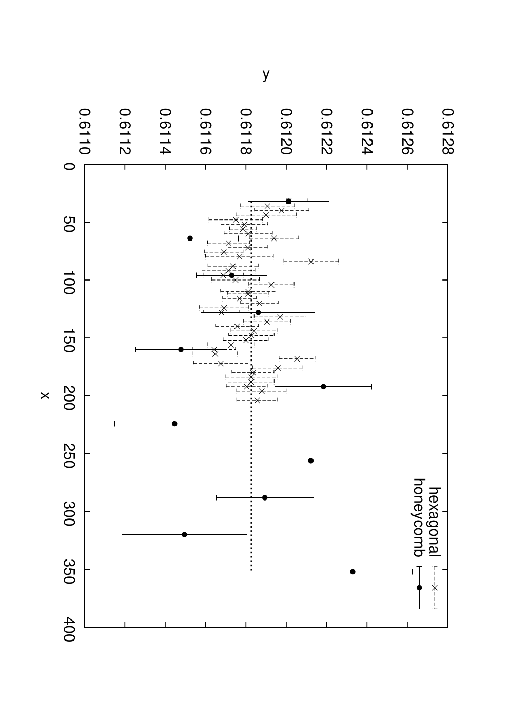
| (50) |
which involves the second and fourth moments of the magnetization , see Fig. 7. The definition of this parameter is such that for a Gaussian theory it vanishes. The critical value of the Binder parameter of the Ising model on a hexagonal lattice with periodic boundary conditions is known extremely well from transfer matrix calculations [31], viz. . Having no scaling dimension, does not change with lattice size in leading order. One-parameter fits to the data lead to the estimates with for the loop gas on the honeycomb lattice (transcribed to the hexagonal lattice), and with for the standard spin representation on the hexagonal lattice. Both estimates, based on different representations of the Ising model and obtained using different update algorithms, are in excellent agreement with the high-precision result.
We next turn to estimators of physical observables which exploit the nature of the worm update algorithm and which can be naturally measured in this scheme. As first estimator we introduce the binary variable that records whether a loop configuration can be mapped onto a spin configuration on the dual lattice, or not. If a map exists, this observable is assigned the value zero, else it is assigned the value unity. The top panel in Fig. 8 shows the average of this observable as a function of the inverse dual temperature introduced in Eq. (47) on lattices of linear extent .


For large , where mostly only a few small loops are present, loop configurations can typically be mapped onto spin configurations on the dual lattice and is small, tending to zero in the limit . When is lowered, larger loops appear and eventually loops can be found that wind around the lattice. As mentioned above, when, for example, a single loop does so once, a transcription is impossible, and the value unity is recorded in the time series of measurements. This explains the increase of with decreasing . In the limit , where loops are abundant, this observable is seen to tend to an asymptotic value (very close to) . In words, the ratio of the number of loop configurations with an odd winding number to those with an even winding number tends to in the zero-temperature limit, where it is recalled that, although impossible for loop configurations with an odd winding number, configurations with an even winding number can be mapped onto a spin configuration on the dual lattice. The observable has no scaling dimension and plays a role similar to the Binder parameter. Finite-size scaling implies that it depends not on the inverse temperature and the lattice size independently, but only on the combination , with the correlation length exponent. The bottom panel in Fig. 8, which displays the same data, but now as a function of this scaling variable with , shows that finite-size scaling is satisfied.
To quantify this statement, we measured at the critical point on lattices of different size, see inset of Fig. 9. A one-parameter fit to the data leads to the estimate with . That is, half of the critical configurations have an odd winding number. Since depends only on the scaling variable , differentiation of with respect to allows estimating , see Fig. 9. A two-parameter fit to the data gives as estimate for the slope with , in excellent agreement with the expected value .

As mentioned above, the great virtue of the worm algorithm is that it also generates open chains. Figure 10 shows the distribution , introduced in Eq. (7), of chains of steps with arbitrary end-to-end distance measured at the critical point on a lattice of linear size . By Eq. (12) and the definition of the magnetic susceptibility in terms of the correlation function given below Eq. (14), the sum gives at the critical point. According to finite-size scaling, scales with lattice size as
| (51) |
The inset of Fig. 10 shows a log-log plot of the ratio as a function of the lattice size. A linear two-parameter fit to the data gives the estimate with , in agreement with the exact result .

An important characteristic of the chains generated by the worm algorithm, whether closed or open, is their Hausdorff, or fractal, dimension . Figure 11 shows the average square radius of gyration of closed and open chains as a function of , as well as the average square end-to-end distance of open chains, also as a function of . In obtaining an accurate estimate of the fractal dimension from these and corresponding data measured on lattices of different size, we face two restrictions. The first is that the scaling (2) only holds asymptotically, i.e., for sufficiently large . To lift this restriction somewhat, we include the leading correction to scaling in Eq. (2) by writing
| (52) |
As for SAWs [32], we expect this leading correction term to be analytic and inversely proportional to . The length of a chain is, on the other side, bounded by the number of lattice sites available on a finite lattice. Figure 10 shows that, as a result, even at the critical point, the number of open chains of arbitrary end-to-end distance falls exponentially for large on a finite lattice. To obtain an estimate for the infinite lattice, chains that exceed a maximum length where they start to notice the finite extent of the lattice must be ignored. As measure of this maximum, we take the length of the shortest polygon winding the lattice recorded in the time series, see Table 3. To be on the safe side, the maximum value of included in the data considered for fitting is chosen to be about , while the minimum value it taken to be .
160 1.485(84) 1.080(61) 0.424 1.43(14) 1.04(10) 0.682 192 1.4213(62) 1.033(19) 0.493 1.475(46) 1.073(33) 0.588 224 1.3822(96) 1.0052(70) 0.301 1.381(16) 1.004(11) 0.288 256 1.3672(67) 0.9943(49) 0.499 1.364(12) 0.9924(90) 0.453 288 1.3762(44) 1.0008(32) 0.867 1.3733(79) 0.9987(58) 0.624 320 1.3738(34) 0.9991(24) 0.850 1.3733(67) 0.9988(49) 0.791 352 1.3755(31) 1.0004(23) 0.697 1.3789(55) 1.0028(40) 0.985 1.3747(19) 0.9998(14) 1.3752(35) 1.0002(25)
Table 4 summarizes the estimates for the fractal dimension obtained through three-parameter fits using the form (52). The last line in the table gives the weighted average of the estimates for , which are all consistent with a constant, i.e., -independent value. The final results are in excellent agreement with the exact value predicted by Saleur and Duplantier [33]. Drawing on numerical work by Cambier and Nauenberg [34], Vanderzande and Stella [35] provided early indirect support for this prediction. Direct numerical support was first provided by Dotsenko et al. [36], and more recently in Ref. [10] using other, percolationlike estimators and a plaquette update.

Polygons that wind the lattice have been excluded from the above measurements. However, as in percolation theory, the fractal dimension of polygons (clusters) at the critical point can also be determined by exclusively focussing on such winding polygons (percolating clusters). Because these polygons are long, no corrections to scaling as in Eq. (52) need to be included. Figure 12 shows the average length of loops winding the honeycomb lattice as a function of lattice size .

A linear fit to the data obtained on lattices of size up to using yields with , in excellent agreement with the predicted result. Note the extra digit of precision achieved here in comparison to the above estimates.
In Fig. 13, we show the probability that one or more loops wind the lattice of size at the critical point. The data show no finite-size effects. A one-parameter fit to the data with ranging from up to gives with . This probability is slightly larger than the probability of finding a configuration with odd winding number because also includes configurations with (nonzero) even winding number.

To detail this further, we give in Table 5 the probability of finding a configuration with winding number measured on lattices of sizes and at the critical point and also in the low-temperature phase at with ()
| (53) |
defining the low-temperature branch of the O() model on a honeycomb lattice [16]. At this temperature, the bond fugacity becomes unity for the Ising model so that each configuration carries the same weight according to the partition function (42). The loop model thus reduces to a purely geometric random model where a bond update is always accepted. By Eq. (47), this temperature corresponds to vanishing inverse dual temperature of the Ising model on the dual lattice where spins are oriented up or down at random. In this limit, the dual model becomes equivalent to random site percolation at the percolation threshold , and the polygons on the honeycomb lattice denote the boundaries of the occupied sites on the hexagonal lattice [33].
0 0.48747(89) 0.48802(74) 0.15764(29) 0.15836(29) 1 0.50029(88) 0.49960(73) 0.74579(34) 0.74545(53) 2 0.01221(12) 0.01236(14) 0.09214(16) 0.09171(36) 3 0.0000307(70) 0.0000299(64) 0.004369(70) 0.004413(76) 4 0 0 0.0000588(64) 0.000060(11)
For the two lattice sizes considered, we have not recorded any configuration with winding number . For the critical theory, we did not even observe a single configuration with . The data show no finite-size effects. The sum of the measured probabilities with odd equals for and for in the case of the critical theory, and for and for at . Since these numerical results are perfectly consistent with the fractions and , it is tempting to speculate that these are in fact exact results.
As final observable, we consider the distribution function of the end-to-end distance introduced in Eq. (8). The top panel in Fig. 14 shows this distribution as a function of for chains of length , and measured on the largest lattice considered, viz. . Each of the distributions are normalized according to Eq. (10) with . If our finite-size scaling conjecture (8) holds for the O(1) loop gas, the data for various should collapse onto a universal curve when with and is plotted as a function of the scaling variable . This is indeed what we observe, see bottom panel in Fig. 14. The analyses of data measured on smaller lattices, typically with three equidistant chain lengths, give similar results. For SAWs it has been suggested [37] that the whole scaling function can be approximated by a single function
| (54) |
with parameters and . This scaling function slightly generalizes the form originally proposed by Fisher [15], where was assumed. The exponent is related to the fractal dimension of the SAWs by the Fisher law [15]
| (55) |
We have cast this law in a form that allows generalization to arbitrary critical O() loop gases, where it is recalled that for SAWs, which are described by the O() model, with , but for arbitrary , . With given the predicted value for , a three-parameter fit to the data yields a surprisingly good approximation of the entire scaling function, see Table 6. The resulting estimate for is in excellent agreement with the predicted value . Note that the normalization (10) translates into the normalization
| (56) |
of the scaling function. With the explicit form (54), this gives a relation between the three parameters , and . Our estimates for these parameters satisfy this relation within statistical errors, so that the fits effectively involve only two free parameters.


160 1.017(08) 3.819(18) 0.3970(73) 1.058(19) 1.80 192 0.992(11) 3.798(24) 0.377(10) 1.006(27) 2.74 224 1.0070(94) 3.820(19) 0.3835(85) 1.022(22) 2.31 256 1.0019(59) 3.815(12) 0.3793(56) 1.011(15) 1.48 288 1.0022(50) 3.807(10) 0.3799(47) 1.013(12) 1.35 320 0.9950(47) 3.790(10) 0.3733(44) 0.995(11) 1.35 352 0.9973(51) 3.814(10) 0.3721(46) 0.992(12) 1.53 0.9994(26) 3.8096(55) 0.3769(24) 1.0050(64)
6 Outlook and discussion
The worm algorithm may potentially turn the loop gas approach to fluctuating fields on a lattice into a viable alternative for numerically simulating lattice field theories. Being an alternative, the algorithm calls for new estimators of physical observables, a few of which we have described here. Up to now, the loop gas approach has been widely adopted only in the de Gennes limit of the O() model, which describes self-avoiding random walks. As demonstrated in this paper, concepts developed to describe such random walks can be generalized to arbitrary O() models. A next step in advancing the worm algorithm, which we hope to explore in a future publication, is to include gauge fields. Finally, although field theories that contain fermions can also be expanded in a strong-coupling series, and are in principle amenable to the worm algorithm, it is an open question whether the algorithm can deal with the sign problem. A first step towards this problem, to which we also hope to return in a future publication, is to simulate the critical O() model for on a honeycomb lattice, so that according to the HT representation (42) each polygon caries a minus sign. That is, in this particular representation, the O() model exhibits the sign problem in its pristine form.
Acknowledgement
Work supported in part by the Deutsche Forschungsgemeinschaft (DFG) under grant No. JA483/23-2 and the EU RTN-Network ‘ENRAGE’: “Random Geometry and Random Matrices: From Quantum Gravity to Econophysics” under grant No. MRTN-CT-2004-005616.
References
- [1] R. P. Feynman, Rev. Mod. Phys. 20, 367 (1948).
- [2] H. E. Stanley, Introduction to Phase Transitions and Critical Phenomena (Oxford University Press, New York, 1971).
- [3] B. Berg and D. Foerster, Phys. Lett. B 106, 323 (1981).
- [4] C. Dasgupta and B. I. Halperin, Phys. Rev. Lett. 47, 1556 (1981).
- [5] W. Helfrich and W. Müller, in Continuum Models of Discrete Systems (University of Waterloo Press, Waterloo, Ontario, Canada, 1980), p. 753. See also F. Rys and W. Helfrich, J. Phys. A: Math. Gen. 15, 599 (1982).
- [6] M. Karowski, H. J. Thun, W. Helfrich, and F. S. Rys, J. Phys. A: Math. Gen. 16, 4073 (1983); M. Karowski and F. S. Rys, J. Phys. A: Math. Gen. 19, 2599 (1986).
- [7] T. Hofsäss, W. Janke, and H. Kleinert, Phys. Lett. A 105, 463 (1984); W. Janke and H. Kleinert, Phys. Lett. A 128, 463 (1988).
- [8] V. Elser, Topics in Statistical Mechanics, Ph.D. Thesis, University of California, Berkeley (1984).
- [9] N. Prokof’ev and B. Svistunov, Phys. Rev. Lett. 87, 160601 (2001).
- [10] W. Janke and A. M. J. Schakel, Nucl. Phys. B [FS] 700, 385 (2004).
- [11] W. Janke and A. M. J. Schakel, Phys. Rev. Lett. 95, 135702 (2005).
- [12] D. Stauffer and A. Aharony, Introduction to Percolation Theory, 2nd edition (Taylor & Francis, London, 1994).
- [13] B. Nienhuis, in: Phase Transitions and Critical Phenomena, edited by C. Domb and J. L. Lebowitz (Academic, London, 1987), Vol. 11, p. 1.
- [14] P. G. de Gennes, Phys. Lett. A 38, 339 (1972).
- [15] M. E. Fisher, J. Chem. Phys. 44, 616 (1966).
- [16] B. Nienhuis, Phys. Rev. Lett. 49, 1062 (1982).
- [17] C. Vanderzande, J. Phys. A: Math. Gen. 25, L75 (1992).
- [18] I. Jensen, J. Phys. A: Math. Gen. 37, 5503 (2004).
- [19] J. des Cloizeaux, Phys. Rev. A 10, 1665 (1974).
- [20] P. G. de Gennes, Scaling Concepts in Polymer Physics (Cornell University Press, Ithaca, 1979).
- [21] D. S. McKenzie and M.A. Moore, J. Phys. A: Math. Gen. 4, L82 (1971).
- [22] N. Prokof’ev and B. Svistunov, Phys. Rev. Lett. 96, 219701 (2006).
- [23] J. Smit, Introduction to Quantum Fields on a Lattice (Cambridge University Press, Cambridge, 2002).
- [24] E. Domany, D. Mukamel, B. Nienhuis, and A. Schwimmer, Nucl. Phys. B 190, 279 (1981).
- [25] L. Chayes, L. P. Pryadko, and K. Shtengel, Nucl. Phys. B 570, 590 (2000).
- [26] C. Gabriel, Dynamical properties of the worm algorithm, Diplomarbeit, Technische Universität Graz (2002).
- [27] U. Wolff, Nucl. Phys. B 810, 491 (2009).
- [28] H. A. Kramers and G. H. Wannier, Phys. Rev. 60, 252 (1941).
- [29] R. H. Swendsen and J. S. Wang, Phys. Rev. Lett. 58, 86 (1987).
- [30] R. B. Potts, Phys. Rev. 88, 352 (1952).
- [31] G. Kamieniarz and H. W. J. Blöte, J. Phys. A: Math. Gen. 26, 201 (1993).
- [32] S. Caracciolo, A. J. Guttmann, I. Jensen, A. Pelissetto, A. N. Rogers, and A. D. Sokal, J. Stat. Phys. 120, 1037 (2005).
- [33] H. Saleur and B. Duplantier, Phys. Rev. Lett. 58, 2325 (1987).
- [34] J. L. Cambier and M. Nauenberg, Phys. Rev. B 34, 8071 (1986).
- [35] C. Vanderzande and A. L. Stella, J. Phys. A: Math. Gen. 22, L445 (1989).
- [36] V. S. Dotsenko, M. Picco, P. Windey, G. Harris, E. Martinec, and E. Marinari, Nucl. Phys. B 448 [FS], 577 (1995).
- [37] J. des Cloizeaux and G. Jannink, Polymers in Solution: Their Modelling and Structure (Oxford University Press, Oxford, 1989).