Some conjectures on the zeros of approximates to the Riemann -function and incomplete gamma functions
Abstract
Riemann conjectured that all the zeros of the Riemann -function are real, which is now known as the Riemann Hypothesis (RH). In this article we introduce the study of the zeros of the truncated sums in Riemann’s uniformly convergent infinite series expansion of involving incomplete gamma functions. We conjecture that when the zeros of in the first quadrant of the complex plane are listed by increasing real part, their imaginary parts are monotone nondecreasing. We show how this conjecture implies the RH, and discuss some computational evidence for this and other related conjectures.
1 Introduction
Following Riemann (as described in a copy of an English translation of his memoir contained in the appendix of [Edw01]), let
| (1) |
is an even, entire function, and the famous Riemann Hypothesis (RH) says that all the zeros of are real. Let denote the first quadrant of the complex plane . Since is even and real on the real line, we can restate the RH as saying all zeros of in are real. Since is nonzero in , it follows that all zeros of in satisfy . In Hardy (as reprinted in [BCRW08]) showed that has infinitely many real zeros and in Selberg [Sel42] showed that a positive proportion of the zeros of are real. More recent work of Conrey [Con89] has at least of the zeros on the real line.
Riemann derived the following expression for ;
| (2) |
where with
| (3) |
The function is known to be an even function of . Pólya [Pól26] investigated ways of approximating by simpler functions. He showed that if in (2) we replace by
| (4) |
(obtained by replacing most of the exponentials in the definition of by hyperbolic cosines), then the resulting integral has only real zeros. Pólya also showed that if we replace by any function which is not an even function of , then the resulting integral has only finitely many real zeros. Hejhal [Hej90] investigated what happens if we replace by a “Pólya approximate”, i.e. a finite sum of the form
| (5) |
By building on earlier work of Bombieri and Hejhal [BH87], which showed that, under the Generalized Riemann Hypothesis (GRH) and some other assumptions, certain linear combinations of Dirichlet -series asymptotically have of their zeros on the critical line, Hejhal was able to show that if we replace in (2) by a Pólya approximate the resulting function asymptotically also has of its zeros on the real line (but infinitely many zeros off the line). By asymptotically we mean that the proportion of zeros in satisfying that are on the real line approaches as .
The starting point for this investigation is the idea that perhaps it is not necessary for worthwhile approximates to have all their zeros on the real line. If a given family of approximates approach uniformly, and if for each element in the family one could prove that within a certain sub-region of all the zeros are real, with the size of the sub-region expanding to eventually include all of as our approximates approach , then this would also imply RH. Thus it may be worth studying replacements for in (2) which are not even. With this in mind, a natural question to ask is what happens if we replace by .
2 Preliminary calculations
Let denote the integral
| (6) |
where , with . Making the change of variable , so , and , we get
| (7) | ||||
| (8) | ||||
| (9) | ||||
| (10) |
where
| (11) |
is the (upper) incomplete gamma function. For lack of a better name, we will refer to as a “hyperbolic gamma function”.
| (12) |
the interchange in integration and summation being justified by the uniform convergence. For , , the function is entire (as a function of ), and hence so is . There is a routine in Maple to compute , and (in the RootFinding package) a routine to compute the zeros, using the argument principle and Newton’s method, of a given analytic function in any rectangle of the complex plane. Using this, the author made several computations to compute the zeros of the -approximates
| (13) |
where
| (14) |
for various small values of . Lists of zeros for some of these are contained in the Appendix. In these computer runs, the parameter “Digits” in Maple (which tells the computer to use this many significant digits in all calculations) was typically set to or so, whatever number of digits was needed to compute the function in question over the specified rectangle accurately to or so significant digits. After runs were made first with Digits equal to , they were sometimes run again with Digits equal to , and the resulting zeros typically agreed to at least decimal digits or so, which the author has taken to mean the computer generated zeros (for Digits equal to ) agree with the actual ones to at least decimal digits, although no attempt has been made to establish rigorous error bounds.
We say that a given function has monotonic zeros in a region of the complex plane if, when we list the zeros of in by increasing real part, the imaginary parts of the zeros are monotone nondecreasing. Formally, if are the zeros of in numbered so that for , then . (We assume has at most one zero on the intersection of any vertical line with .) The data in the Appendix and other computer runs support the following hypothesis.
Conjecture 1
For , has monotonic zeros in .
Proposition 1
Conjecture 1 implies the Riemann Hypothesis.
Proof. This follows from the argument principle, combined with the simple fact that a function with infinitely many positive real zeros, and with monotonic zeros in , has only real zeros in . Assume the RH is false, and let be the zero of in with minimal real part, among those zeros with positive imaginary part, and let . By the argument principle, we have
| (15) |
where the integral is taken counterclockwise around a circle centered at , of small radius , so no other zeros of are enclosed in . Next choose sufficiently large so that has a real zero with . We can do this since converges uniformly to on compacta in , both and are real on the real line, and since has infinitely many positive real zeros. By assumption has monotonic zeros in , hence has no non-real zeros in with real part less than . This implies
| (16) |
and so
| (17) | ||||
| (18) |
On the closed and bounded set , is nonzero and hence must assume an absolute minimum . Due to the uniform convergence, as , the minimum of on must eventually be greater than . Hence for large the modulus of the denominator of the integrand in (18) is bounded away from zero, but (since approaches uniformly) the numerator approaches zero, and so the integral will also approach zero, a contradiction.
Remark 1
A weaker form of Conjecture 1, which still implies RH, is that there are no non-real zeros of in whose real part is less than the largest real zero of . Since is real for real , the real zeros can be found by looking at sign changes along the real line. Then the argument principle can be used via a numerical integration to obtain the total number of zeros of with real part not greater than the largest real zero, and matched against the number of real zeros. Computations along these lines indicate this weaker form of Conjecture 1 is true at least for . Below we list the largest real zero and number of real zeros of for .
3 Other Zeta Functions
Many other zeta functions which are conjectured to satisfy a Riemann Hypothesis can be approximated by sums of hyperbolic gamma functions. Let denote Ramanujan’s -function. Since the function
| (19) |
is a modular form of weight , we have
| (20) |
which can be used to show
| (21) |
which implies
| (22) |
again a uniformly convergent sum of hyperbolic gamma functions. (It is known that [Apo90].) The function defined by the left-hand-side of (22) is known as the Ramanujan -function, which we denote , and the approximate obtained by truncating the series on the right-hand-side of (22) after steps we denote . Ramanujan conjectured that has only real zeros, which is still open. We mention that Ki [Ki08] has studied the zeros of different approximates to the Ramanujan -function.
Conjecture 2
For , has monotonic zeros in .
Computations analogous to those described in Remark 1 indicate that the corresponding weaker form of Conjecture 2, that there are no nonreal zeros of in with real part smaller than the largest real zero of , is true at least for . Below we list the number of real zeros and the largest real zero of for .
More generally, we can start with any entire modular cusp form
| (23) |
of weight , and set
| (24) |
The modularity of can be used to show [Apo90, pp. 137-138] that
| (25) | ||||
| (26) |
where we have used the well-known bound to justify the interchange of summation and integration. Thus we see that, at least for even, is also a uniformly convergent (infinite) linear combination of hyperbolic gamma functions.
We can do a similar calculation for Dirichlet L-series with a primitive character with modulus . Assume for the moment that , and define
| (27) |
From [Dav00, pp.68-69] we have (using the fact that )
| (28) | ||||
| (29) | ||||
| (30) | ||||
where is a certain complex number of modulus one and is the conjugate character. Furthermore if we get
| (31) | ||||
| (32) | ||||
| (33) | ||||
| (34) | ||||
where again .
Let be the function defined by truncating the series on the right-hand-side of (26), or both of the series on the right-hand-side of either (30) or (34), after steps. If Conjectures and 1 and 2 are true, one might suspect that also has monotonic zeros in , although the author has not yet done any computations with these more general sums.
Another interesting question is where the zeros of are, for a positive real number. Neilsen [Nie65] showed that has no zeros in , and Gronwall [Gro16] proved that has infinitely many zeros in . Mahler [Mah30] showed that, as , the zeros of cluster about the limiting curve
| (35) |
Tricomi and other authors have investigated the zeros of (the meromorphic continuation of) as a function of , for fixed . In summary, not much information seems to be known about the zeros of , for a fixed positive real number ( although the literature contains a number of detailed results on the zeros of the lower incomplete gamma function ). In Gautschi [Gau98] published a nice survey of known results on incomplete gamma functions.
Computer calculations support the following.
Conjecture 3
For any fixed positive real number , the incomplete gamma function has monotonic zeros in .
Although some analog of Conjecture 3 may be true for hyperbolic gamma functions, in Section 5 we show that there exist some choices of , for which does not have monotonic zeros in .
Remark 2
To say a function has monotonic zeros in is equivalent to saying that the first differences of the imaginary parts of the zeros are all nonnegative. The zeros in of seem to satisfy the more general property that the -th differences of the imaginary parts of the zeros are positive for odd and negative for even, for or . Thus these zero sets seem to have extra structure beyond being monotonic. For linear combinations of hyperbolic gamma functions the same phenomena seems to occur for sufficiently large, which may be due to the main term in the asymptotics controlling the zeros.
4 Asymptotics
Throughout this section , , , . We begin with Stirling’s formula and some other known results:
| (36) |
(where )
| (37) |
([EMOT53, Vol. II, p. 135])
| (38) |
([EMOT53, Vol. I, p. 47]), where in the big-Oh results we mean as . From (36) we see that
| (39) |
Now if and only if so by (37) , large implies
| (40) |
or
| (41) |
If remains bounded and , the left hand side above grows too fast, while if remains bounded and it decreases too fast. Hence we need both . Furthermore, must be asymptotic to , hence and the zeros of in satisfy as .
To perform the same analysis for , first note that
| (42) | ||||
| (43) |
Thus using (38),
| (44) | ||||
| (45) |
From (37),
| (46) | |||
One finds
| (47) | |||
If remains bounded and doesn’t, then the first two terms on the right-hand-side of (46) approach like , so by (47), the expansion of in negative powers of has a nonzero coefficient of , unless in which case it has a nonzero coefficient of . In either case it cannot equal for sufficiently large . If remains bounded and doesn’t, then the second term on the right-hand-side of (46) blows up, while the others approach . So as , for fixed , if we need both , and thus from (45) cannot approach positive or negative infinity too quickly. In fact the zeros of must satisfy as .
The argument above also applies to any function of the form
| (48) |
, i.e. any -linear combination of hyperbolic gamma functions. For if you have a linear combination of terms like (46), more than one of which is approaching , the linear combination must also approach , since by taking into account the contribution of , no two such terms can approach at the same rate. The other parts of the argument follow through similarly (the coefficient of in the appropriate version of (47) must be nonzero for some , else (48) would essentially reduce to a linear combination of Gamma functions, which would not be entire) and thus the zeros of any function of the form (48) also satisfy as .
5 Linear Combinations
The examples in Section 3 involving Dirichlet characters motivate defining, for , , , , the generalized hyperbolic gamma function as
| (49) |
The author has made several hundred computer runs, calculating the zeros of various arbitrary -linear combinations of generalized hyperbolic gamma functions in different regions of . Surprisingly, in all of these runs the zeros turned out to be monotonic. Perhaps this results from a mysterious analytic principle, not yet understood, which causes generic sums of generalized hyperbolic gamma functions to have a high probability of having monotonic zeros. In this case the RH could be a consequence of this analytic principle, combined with Hardy’s theorem that has infinitely many real zeros.
It is not the case though that all linear combinations of generalized hyperbolic gamma functions have monotonic zeros in . For example, consider any function of the form , where are positive real numbers and are any two -functions, corresponding to different zeta functions from Section 3, which are real on the real line. Since and have infinitely many real zeros, as along the real line they each oscillate from positive to negative. Unless there is an unsuspected correlation between the two, any real linear combination of them will also oscillate and thus have infinitely many real zeros. But only for very special choices of will this linear combination correspond to a zeta function with an Euler product, and without an underlying Euler product it is generally expected that such functions will have infinitely many non-real zeros as well. In particular, , the sum of the Riemann -function and the fifth approximate to the Ramanujan function, has a non-real zero with real part between 19 and 23, and a real zero at . (Here is evaluated at to make the two functions compatible, since the expression (12) of in terms of hyperbolic gamma functions involves , while that of involves .)
More simply, one can create an example of non-monotonic zeros by considering what happens to as along the positive real line. From (46) and (47) we get
| (50) |
Applying this to (13) yields
| (51) |
which shows
| (52) | ||||
For the coefficient of in is positive. Thus the coefficient of in is positive for and negative for . It follows that is positive for sufficiently large if and negative for sufficiently large if , and so has a zero on the real line for some large and some . One finds in fact that there is a real zero between and when , which occurs after many non-real zeros, giving an example of non-monotonic zeros. This real zero travels travels quickly left as increases through real values, arriving at (the largest real zero of ) when .
One could hope that any series of the form
| (53) |
has monotonic zeros, modulo the problem of the forced real zero described above, which could be avoided by say requiring , since then
| (54) |
for some . A family of polynomials with real coefficients is called compatible if
| (55) |
has only real zeros whenever for . It is called pairwise compatible if forms a compatible family for each pair . Chudnovsky and Seymour [CS07] have shown that a family of polynomials whose members have only real zeros and positive leading coefficients is compatible if and only if it is pairwise compatible. Does a similar statement hold if we replace real polynomials with positive leading coefficients and only real zeros, by even, real, entire functions having monotonic zeros in ?
Eq. (50) also leads to an example of a single hyperbolic gamma function with non-monotonic zeros. For very large clearly and , so there must be some value of , for which for some very large , which will thus have non-monotonic zeros in .
Another interesting phenomena occurs when we consider the zeros of . As we let vary continuously from to , computations indicate that the imaginary parts of the non-real zeros decrease monotonically (i.e. continuously), in a very regular manner, until, for high enough , they collide with the corresponding zero (from Schwartz reflection) in the fourth quadrant, and arrive on the real line, where they remain.
Conjecture 4
For , the imaginary part of each non-real zero of decreases monotonically (i.e. continuously) as goes from to .
6 The modulus on vertical rays
It is known that the RH is equivalent to the statement that the modulus of is monotone increasing along any vertical ray which starts at a point on the nonnegative real line and travels straight upward to . (Clearly if the RH is false the statement is false. On the other hand, if the RH is true, start with Hadamard’s factorization theorem
| (56) |
where the are the positive real zeros of , and take the partial derivative with respect to , where . This is easily seen to be positive for positive .)
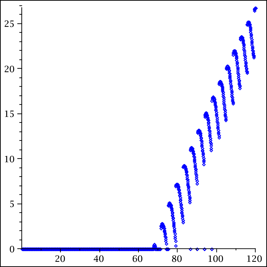
For a given function , analytic in , and a nonnegative real number, let denote the value of where the function is minimal, i.e. the height where the minimum of the modulus of occurs on the vertical ray starting at and going straight up. (If this minimum occurs at more than one , let denote the lim inf of such .) Finally call the set of pairs in the “M-curve” of .
Examples of these curves are given in Figures 1, 2, and 3 below. To calculate for a given pair and the author simply calculated the modulus of at many closely spaced grid points and then chose the which gave the minimum of these numbers (from the asymptotics, the modulus of a sum of hyperbolic gamma functions increases quite rapidly when increases beyond a certain point). This same procedure was followed for several closely spaced grid points , and the pairs then plotted on a grid using Maple, with the result looking something like a continuous curve. They seem to have the (as yet unexplained) property that the non-real zeros of in occur at the same places as the local maxima of the M-curve. If so, this would give another (rather informal) method for calculating the zeros of and other sums of hyperbolic gamma functions which doesn’t depend on the argument principle or Newton’s method. Other computations indicate this property may also hold for any real polynomial with no two zeros in the upper half-plane with the same real part.
6.1 Some Notes on the Computations
The list of zeros of in the Appendix was calculated using the argument principle and Newton’s method by a call to the function analytic in Maple, as were the zeros of , , and the zeros of the sum of two generalized hyperbolic gamma functions. This procedure failed however to compute the zeros of , as the program never finished even after running for over two days on the Sun system at the University of Pennsylvania. Note that is a sum of incomplete gamma functions, which may explain why the computation of the zeros of quickly becomes difficult. The author was able to find the zeros of by starting with the zeros of and using Newton’s method to find the zeros of , for a small positive number, then recursively using these new zeros and Newton’s method to find the zeros for a slightly larger value of , slowly increasing until equaled . The author then tried to compute the zeros of in the same way, by starting with the zeros of and using Newton’s method to compute the zeros of for small , and gradually increasing as before. This worked well until became very close to , about , at which point Newton’s method no longer converged. If the property discussed in the previous paragraph holds though, we can see from Figure 2 where the non-real zeros of in the range are.


7 Appendix
, zeros of first -approximate in rectangle with corners .
14.04543957882981756479858,
20.62534600592171760132974 + 2.697151842339519632505712 I
26.05616693357829946749575 + 7.125359707612690330897455 I
31.50143137824977099308422 + 10.72915037105496782822450 I
36.72702276874255239918647 + 13.75961410603683555833019 I
41.73703479849622101486046 + 16.44012737324329251859479 I
46.56622866997881255099908 + 18.88186965378958902053812 I
51.24456582311629453468990 + 21.14750420601374895347492 I
55.79525368022472028456165 + 23.27625685820891335493023 I
60.23621426525993802296865 + 25.29458549895993860216014 I
64.58150497097301796850798 + 27.22133555778112035831075 I
68.84235653395121330563843 + 29.07049609150585601287785 I
73.02789933182939276748060 + 30.85279227139366634464017 I
77.14567324003250763696303 + 32.57666324204392832752644 I
81.20199121212953110713480 + 34.24889253114939152723783 I
85.20220345212231662722890 + 35.87503096670553315342957 I
89.15089297349449318064800 + 37.45968995259880236581690 I
93.05202292717284600209187 + 39.00675061925213970478000 I
96.90904939663401491219210 + 40.51951660155401879741380 I
1st differences of imaginary parts of zeros
2.697151842339519632505712
4.428207865273170698391743
3.603790663442277497327045
3.03046373498186773010569
2.68051326720645696026460
2.44174228054629650194333
2.26563455222415993293680
2.12875265219516440145531
2.01832864075102524722991
1.92675005882118175615061
1.84916053372473565456710
1.78229617988781033176232
1.72387097065026198288627
1.67222928910546319971139
1.62613843555614162619174
1.58465898589326921238733
1.54706066665333733896310
1.51276598230187909263380
, zeros of in rectangle with corners .
14.1347251016150223590867934323428320
21.0220425550989420016995644399118565
25.0108186655252580507941448128443705
30.4267684045343046403275534114141879
32.9244008910878391337889771099093884
37.8603410698702633339745855804483258
39.5324810797879508571153350051479630
43.1389080680988950956236929709951507 + 3.28097100306881350163884998294539870 I
47.5227563037011494043923449534796642 + 6.25250911174970354129046143001000600 I
51.8283147335875594556295444210165891 + 8.95857384762622450769949019637180856 I
56.1120029199774070873341435705058778 + 11.4796085175258061625014962442075566 I
60.3502919249623580499827793888173447 + 13.8416168548275384327656057308155260 I
64.5390675686875954205140494065924195 + 16.0705629583418306170962131727661418 I
68.6761126675575950561373116041091163 + 18.1868197094425056650011185673044960 I
72.7617836933667997393215687715081074 + 20.2066697023948159796720721861483021 I
76.7975312791721943222372025862518267 + 22.1432248556299027619859319905393103 I
80.7854051988095067379835000872591797 + 24.0071081808438939881307280663316996 I
84.7277019646143359935370107950650673 + 25.8070157111458796320542608491379890 I
88.6267772741056992788936274593068783 + 27.5501321650503597200806915781312903 I
92.4849402660525200867715711075727066 + 29.2424518834035459512085274002314648 I
96.3043979005927443711172685790765488 + 30.8890225459009695084228517057586202 I
100.087228624602886284768301012877784 + 32.4941324878154139135000560357642324 I
, zeros of in rectangle with corners .
14.13472514173469376946955013374227983392383419451107438
21.02203963877155659023693964971327708279243073624430253
25.01085758014566673273814860967472222032345345332059477
30.42487612586063748020316156144982639562443306193294638
32.93506158773265354499645423632051649764195395468931578
37.58617815896445021695716617231461056957864550061946742
40.91871901006637538924149719014594063254432154184503222
43.32707329088964789958258005109768490700030014005496697
48.00515051035397786165873118175586051353275737166717210
49.77383399904302558365984997979234680103752864503720614
52.97031190983202078103080161894128897412215226172440818
56.44637829985894482385431963634767652784719134486888209
59.34511184966886217051112646891854833040742035322093409
60.83672336038805375320166674337805885068490701004798353
65.03207377198913910137679883482704065081967504834437506
, zeros of first approximate to the Ramanujan -function in rectangle with corners .
9.5489635091412543125672429455388951 + 1.7119172216212706912355445109132207 I
13.789433051893611052566335275629933 + 5.2848734079809646491896114233647142 I
17.427358570320731571246782104695096 + 7.7540563400814520087583759352815352 I
20.757098189027862070211629799284288 + 9.7974743824676388131629735365802915 I
23.879056232416349736892490077064465 + 11.592456287772395127573044664358961 I
26.847356442625470267126707245453301 + 13.219199923922411333605849186386965 I
29.695457505212671889597523331405240 + 14.722240962151850502838429485181816 I
32.445858241734786458856784110868772 + 16.129361168830359821304709531815352 I
35.114596915766277030958889001310311 + 17.459270918804088444729979963005156 I
37.713610437352047890893961093475018 + 18.725280350575037459960230440611499 I
40.252083817737620602530239123250025 + 19.937256671472885578681886805140642 I
42.737274291251073747956340698712113 + 21.102754510914081337479910411119165 I
45.175041128226087752248534272004155 + 22.227709943351466358153291572887016 I
47.570200654826011921382328419781717 + 23.316887844914435394477534028073124 I
49.926772425743961667810425669964510 + 24.374181909750589494277749519061023 I
52.248154899971609917404551354946461 + 25.402822596146688919661995414148711 I
54.537253919041181821883861911330465 + 26.405525330914909309258552834547793 I
56.796578677359823555284912818063663 + 27.384598689419083619944995509463388 I
59.028314745351122620881979673545968 + 28.342025013215928897705357026998109 I
61.234380542300284878652304849348298 + 29.279521587539252797178004730959225 I
63.416471643946175987038219068629433 + 30.198587816232713426722974287579177 I
65.576095995892802432660080685311982 + 31.100542121402673258701892990637098 I
67.714602225166643613493231218811692 + 31.986551176775085187674532167087986 I
69.833202642000750529879098123320031 + 32.857653335480587110184136136077900 I
71.932992106046633644353345531169636 + 33.714777601864923783681632805009935 I
74.014963635252309537091144416299462 + 34.558759141214355169362183745447748 I
76.080021422732136425762615907263059 + 35.390352069528146990609600601997921 I
78.128991771589170231983397657306861 + 36.210240084528180967081058119582790 I
80.162632342789627094434403795275856 + 37.019045367211828466413017905373453 I
82.181640025246587241041487951836980 + 37.817336085881271861478883874617446 I
84.186657672248860977039557949370316 + 38.605632761831562562091441356062965 I
86.178279898670686132064566105956960 + 39.384413700925457309936759214348925 I
88.157058095044852280187866298051226 + 40.154119653347769812443058137516104 I
90.123504784721498632008498428129335 + 40.915157831527436633928427478875093 I
92.078097426893282987651528394221783 + 41.667905391109706656241503132525470 I
94.021281749721926032933713327889188 + 42.412712460188349826344885668577328 I
95.953474683021781433616191339406534 + 43.149904786473380482490406058490112 I
97.875066948097497309259057547588008 + 43.879786059713960896674731680251557 I
99.786425352756449975929052839495573 + 44.602639956801403127156000977181747 I
, zeros of second approximate to the Ramanujan -function in rectangle with corners .
9.19376894449217893
13.8348516743546257 + 1.54300060155520050 I
17.0006907368319637 + 4.58047657550007841 I
20.1893418670461022 + 6.99896197324829350 I
23.2665587059084961 + 9.04437482423736081 I
26.2157755564237380 + 10.8464634984827865 I
29.0559366154717340 + 12.4806210190923921 I
31.8034718883051467 + 13.9910040730670684 I
34.4718383897903041 + 15.4050720323654861 I
37.0718504676122273 + 16.7414677662025767 I
39.6120959833238977 + 18.0135340186718953 I
42.0994917987503797 + 19.2311725419877171 I
44.5397026159453686 + 20.4019721238147549 I
46.9374285351558464 + 21.5319037938006434 I
49.2966167316589794 + 22.6257645644359874 I
51.6206201858570109 + 23.6874764176583670 I
53.9123161924908609 + 24.7202947836257462 I
56.1741960636482404 + 25.7269571656683657 I
58.4084343572848694 + 26.7097915965161903 I
60.6169430187982438 + 27.6707975724897949 I
62.8014141732518389 + 28.6117075511920988 I
64.9633543292524033 + 29.5340343986557084 I
67.1041120187127688 + 30.4391085162350689 I
69.2249003477575950 + 31.3281072698702158 I
71.3268155548021774 + 32.2020785869307989 I
73.4108524066057312 + 33.0619600720511948 I
75.4779170679704262 + 33.9085946393025650 I
77.5288379348185691 + 34.7427434066455078 I
79.5643748117146020 + 35.5650964167873912 I
81.5852267334967588 + 36.3762816159807758 I
83.5920386687224333 + 37.1768724246086591 I
85.5854072948756678 + 37.9673941604083026 I
87.5658859982298918 + 38.7483295199556847 I
89.5339892223226212 + 39.5201232818472100 I
91.4901962662154965 + 40.2831863625189748 I
93.4349546156253617 + 41.0378993303884662 I
95.3686828755524769 + 41.7846154642047194 I
97.2917733614022269 + 42.5236634258506564 I
99.2045943961865493 + 43.2553496053959862 I
, zeros, in rectangle with corners , of linear combination of two generalized hyperbolic gamma functions
| (57) |
where
| (58) | ||||
| (59) | ||||
| (60) |
10000.08899697917243762827 + 1943.699378898319010297001 I,
10000.84424695361683674126 + 1943.828178641310676925944 I,
10001.59949024766823939791 + 1943.956976210289663002380 I,
10002.35472686200573704240 + 1944.085771605493580928470 I,
10003.10995679730829337130 + 1944.214564827159996509445 I,
10003.86518005425474436858 + 1944.343355875526428966768 I,
10004.62039663352379834061 + 1944.472144750830350951281 I,
10005.37560653579403595119 + 1944.600931453309188556355 I,
10006.13080976174391025650 + 1944.729715983200321331031 I,
10006.88600631205174674006 + 1944.858498340741082293155 I,
10007.64119618739574334772 + 1944.987278526168757942515 I,
10008.39637938845397052261 + 1945.116056539720588273964 I,
10009.15155591590437124002 + 1945.244832381633766790543 I,
10009.90672577042476104237 + 1945.373606052145440516603 I,
10010.66188895269282807412 + 1945.502377551492710010906 I,
10011.41704546338613311658 + 1945.631146879912629379767 I,
10012.17219530318210962295 + 1945.759914037642206290096 I,
10012.92733847275806375302 + 1945.888679024918401982558 I,
10013.68247497279117440814 + 1946.017441841978131284633 I,
10014.43760480395849326601 + 1946.146202489058262623716 I,
10015.19272796693694481556 + 1946.274960966395618040195 I,
10015.94784446240332639171 + 1946.403717274226973200536 I,
10016.70295429103430821021 + 1946.532471412789057410354 I,
10017.45805745350643340246 + 1946.661223382318553627526 I,
10018.21315395049611805021 + 1946.789973183052098475038 I,
10018.96824378267965122043 + 1946.918720815226282254485 I,
10019.72332695073319499999 + 1947.047466279077648958683 I,
10020.47840345533278453047 + 1947.176209574842696284945 I,
10021.23347329715432804280 + 1947.304950702757875648075 I,
10021.98853647687360689210 + 1947.433689663059592193412 I,
10022.74359299516627559224 + 1947.562426455984204809882 I,
10023.49864285270786185070 + 1947.691161081768026142988 I,
10024.25368605017376660312 + 1947.819893540647322607883 I,
10025.00872258823926404804 + 1947.948623832858314402362 I,
10025.76375246757950168151 + 1948.077351958637175519890 I,
1st differences of imaginary parts
0.128799742991666628943
0.128797568978986076436
0.128795395203917926090
0.128793221666415580975
0.128791048366432457323
0.128788875303921984513
0.128786702478837605074
0.128784529891132774676
0.128782357540760962124
0.128780185427675649360
0.128778013551830331449
0.128775841913178516579
0.128773670511673726060
0.128771499347269494303
0.128769328419919368861
0.128767157729576910329
0.128764987276195692462
0.128762817059729302075
0.128760647080131339083
0.128758477337355416479
0.128756307831355160341
0.128754138562084209818
0.128751969529496217172
0.128749800733544847512
0.128747632174183779447
0.128745463851366704198
0.128743295765047326262
0.128741127915179363130
0.128738960301716545337
0.128736792924612616470
0.128734625783821333106
0.128732458879296464895
0.128730292210991794479
0.128728125778861117528
2nd differences of imaginary parts of zeros (times minus )
References
- [Apo90] Tom M. Apostol. Modular functions and Dirichlet series in number theory, volume 41 of Graduate Texts in Mathematics. Springer-Verlag, New York, second edition, 1990.
- [BCRW08] P. Borwein, S. Choi, B. Rooney, and A Weirathmueller. The Riemann Hypothesis. CMS Books in Mathematics. Springer, New York, NY, 2008.
- [BH87] Enrico Bombieri and Dennis A. Hejhal. On the zeros of Epstein zeta functions. C. R. Acad. Sci. Paris Sér. I Math., 304(9):213–217, 1987.
- [Con89] J. B. Conrey. More than two fifths of the zeros of the Riemann zeta function are on the critical line. J. Reine Angew. Math., 399:1–26, 1989.
- [CS07] Maria Chudnovsky and Paul Seymour. The roots of the independence polynomial of a clawfree graph. J. Combin. Theory Ser. B, 97(3):350–357, 2007.
- [Dav00] Harold Davenport. Multiplicative number theory, volume 74 of Graduate Texts in Mathematics. Springer-Verlag, New York, third edition, 2000. Revised and with a preface by Hugh L. Montgomery.
- [Edw01] H. M. Edwards. Riemann’s zeta function. Dover Publications Inc., Mineola, NY, 2001. Reprint of the 1974 original [Academic Press, New York; MR0466039 (57 #5922)].
- [EMOT53] Arthur Erdélyi, Wilhelm Magnus, Fritz Oberhettinger, and Francesco G. Tricomi. Higher transcendental functions. Vols. I, II. McGraw-Hill Book Company, Inc., New York-Toronto-London, 1953. Based, in part, on notes left by Harry Bateman.
- [Gau98] Walter Gautschi. The incomplete gamma functions since Tricomi. In Tricomi’s ideas and contemporary applied mathematics (Rome/Turin, 1997), volume 147 of Atti Convegni Lincei, pages 203–237. Accad. Naz. Lincei, Rome, 1998.
- [Gro16] T. H. Gronwall. Sur les zéros des fonctions et associées à la fonction gamma. Ann. École Norm. Sup., 3(33):381–393, 1916.
- [Hej90] Dennis A. Hejhal. On a result of G. Pólya concerning the Riemann -function. J. Analyse Math., 55:59–95, 1990.
- [Ki08] Haseo Ki. On the zeros of approximations of the Ramanujan -function. Ramanujan J., 17(1):123–143, 2008.
- [Mah30] K. Mahler. über die nullstellen der unvollstaendigen gammafunktionen. Circ. Mat. Palermo, 54:1–31, 1930.
- [Nie65] Niels Nielsen. Die Gammafunktion. Band I. Handbuch der Theorie der Gammafunktion. Band II. Theorie des Integrallogarithmus und verwandter Transzendenten. Chelsea Publishing Co., New York, 1965.
- [Pól26] G. Pólya. Bemerkung Über die Integraldarstellung der Riemannschen -Funktion. Acta Math., 48(3-4):305–317, 1926.
- [Sel42] Atle Selberg. On the zeros of Riemann’s zeta-function. Skr. Norske Vid. Akad. Oslo I., 1942(10):59, 1942.