O-V-S-Z and friends: Non-Gaussianity from inhomogeneous reionization
Abstract
We calculate the cosmic microwave background (CMB) bispectrum due to inhomogeneous reionization. We calculate all the terms that can contribute to the bispectrum that are products of first order terms on all scales in conformal Newtonian gauge. We also correctly account for the de-correlation between the matter density and initial conditions using perturbation theory up to third order. We find that the bispectrum is of local type as expected. For a reasonable model of reionization, in which the universe is completely ionized by redshift with optical depth to the last scattering surface the signal-to-noise ratio for detection of the CMB temperature bispectrum is and confusion in the estimation of primordial non-Gaussianity is . For an extreme model with and we get and .
Keywords:
cosmic background radiation — cosmology:theory — dark ages, reionization, first stars — early universe — inflationI Introduction
Secondary anisotropies [1] in the cosmic microwave background CMB can be used to probe the universe after recombination. It is also important to take them into account when using CMB to learn about the initial conditions of the universe. One important class of secondary anisotropies arises due to the scattering of CMB photons by free electrons during and after reionization. In this class, cosmologists have so far concentrated on only one of the terms in the second order Boltzmann equation, the product of electron velocity and electron number density (). It is known as Sunyaev-Zel’dovich effect when the source of electrons is hot gas in galaxy clusters [32]. If instead of thermal motion velocity due to the bulk motion of electrons is considered it is known as Ostriker-Vishniac (OV) effect [24, 36] or kinetic Sunyaev-Zel’dovich (kSZ) effect. There are however additional terms in the full second order equations [2, 3, 25, 30] which also arise due to scattering of CMB photons by electrons and which might be important. Most of the work on OV/kSZ effect has focused on the CMB power spectrum . The CMB bispectrum and trispectrum were calculated in Castro [7], Castro [8], however they calculated the next to leading order term which is a six point correlation function of first order terms for the bispectrum. The leading order term in bispectrum is a four point correlation function of first order terms. They also ignored the de-correlation between the linear and the non-linear quantities in their calculation.
The CMB bispectrum due to inhomogeneous recombination was calculated in Khatri & Wandelt [17] hereafter referred to as KW09 (see Senatore et al. [31] for a different approach, also Khatri & Wandelt [18]). The same equations need to be solved for inhomogeneous reionization and we will follow the treatment in KW09. We will model the inhomogeneous reionization using the linear perturbation theory of Zhang et al. [37] (hereafter ZHH07). For the recombination case the Doppler terms which give rise to OV/kSZ effects were found to be sub-dominant compared to the net contribution from the quadrupole and higher order moments of the CMB. We will see that this is also the case for reionization. For all calculations the gauge dependent quantities are in conformal Newtonian gauge. The cosmological parameters used are baryon density , cold dark matter density , cosmological constant , number of massless neutrinos , Hubble constant , present CMB temperature , primordial Helium fraction , spectral index of primordial fluctuations and .
II Inhomogeneous reionization
We will use the linear perturbation theory of ZHH07 to model reionization. The results from this model are similar to the bubble model of reionization [12]. Due to the fact that reionization is sourced by non-linear physics, the validity of any model will have to be tested with computer simulations (see Trac & Gnedin [34] for a recent review). For our purpose the analytical treatment of ZHH07, which captures the essential features of reionization on linear scales, is sufficient. We refer the reader to ZHH07 for details of the model as well as for discussion on the validity of this approach. An important input for this theory is a model for the distribution of ionizing sources. We will use the same model used in ZHH07 which is based on the excursion set treatment of halo formation [26, 5, 22] with the minimum mass of a halo given by virial temperature of K corresponding to where hydrogen line cooling becomes efficient. The spectrum of ionizing radiation is taken to be a power law
| (1) |
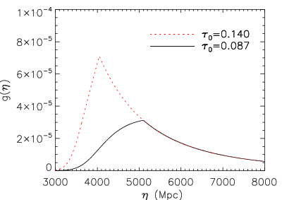
where , is the photon frequency, is the ionization threshold for hydrogen, is the Planck’s constant, is the number of ionizing photons emitted at frequency per unit parameter per collapsed hydrogen atom, is the spectral index of ionizing radiation spectrum, is the total number of ionizing photons emitted per hydrogen atom and is the normalization constant with the spectrum cutoff at . We take into account Helium reionization by assuming that the first ionization of Helium is identical to that of Hydrogen. Although not strictly correct, it should introduce only a small error, unimportant for us, since Helium will contribute only about of the total electrons. Second ionization of Helium is expected to occur at much lower redshifts [11] and will give a negligible contribution to the CMB bispectrum. We will consider two different models of reionization arrived at by choosing different values of parameter in Equation 1 with spectral index . For the first model we choose to give the optical depth to the last scattering surface . For the second model we choose resulting in which can be considered a reasonable upper limit based on WMAP 5 year results [19]. Figure 1 shows the reionization history for these two models. We use the RECFAST code [28] to calculate the residual mean electron number density after recombination switching to reionization code once the electron density due to reionization exceeds the residual value from recombination. The ratio of electron number density perturbation to matter density perturbation for comoving wavenumber of is plotted in Figure 2. We use the approximate solutions to the perturbation equations given in ZHH07 and force the electron bias once the universe is fully reionized. This is a very good approximation to the exact equations of ZHH07 where the bias goes smoothly to unity. The matter density and hence the electron number density will be non-linear on small scales and thus will de-correlate with the linear quantities, for example CMB, on these scales. We will use on all scales, where is calculated using linear theory but can be non-linear. We will take the de-correlation into account using the third order perturbation theory. Note that the non-linearity will be significant only at low redshifts for scales of interest when the universe is fully reionized and exactly. Also for the leading term in the bispectrum we need to correlate CMB with the electron number density perturbation. However this correlation will be small on scales much smaller than the horizon size because CMB traces the perturbations at a much higher redshift than that of reionization. Thus the contributions to the bispectrum from perturbations in the electron number density will be significant only for scales which are linear and where we should expect the linear perturbation theory of reionization to work well.
At low redshifts a significant fraction of baryons are expected to be in a diffuse phase called warm-hot intergalactic medium (WHIM) [9, 10]. The perturbations in these baryons are suppressed on small (non-linear) scales compared to the dark matter and for these baryons the bias should be less than . However the contribution to the bispectrum from is and contribution from is . This is because of the absence of bias due to the inhomogeneities in the reionization process once the universe is completely reionized and the decreasing optical depth due to the expansion of the universe. At only a small percentage of baryons are in WHIM (). Thus their contribution to the bispectrum is less than and the error in assuming negligible. We neglect the contribution from in our numerical calculations.


III Cross correlation between matter density and initial conditions
We will need to calculate the correlation () between the electron number density and linear perturbation variables or equivalently the cross-correlation between the non-linear matter density () and linearly evolved matter density (). We will be interested in the CMB anisotropies on scales of angular wavenumber , corresponding to the smallest scales predicted to be probed by the Planck mission 11 1 http://www.rssd.esa.int/Planck. On these scales it is sufficiently accurate to calculate the next term in the perturbation expansion which, for , means going to the third order in perturbation theory for matter density perturbation . For Einstein-De Sitter universe () the solution for can be written as the following perturbation series [35, 13, 23, 15] (see Bernardeau et al. [4] for a review).
| (2) |
where is the linear matter density perturbation at and is of order , is the Fourier wavenumber and is conformal time. The correlation between the linear and the non-linear matter density is then given by
| (3) | |||||
where is the linear matter power spectrum at and is the correction given by [33]
| (4) | |||||
For a general cosmology replacing the scale factor with the linear growth factor in the Einstein De-Sitter solution gives an excellent approximation to the true result [27, 4]. Thus we have
| (5) |
where is negative signifying de-correlation between the linear and the non-linear density fields as expected.
We plot the ratio of cross power spectrum to linear power spectrum in Figure 3. For , the CMB bispectrum will get contributions from Fourier modes . It is evident from Figure 3 that for the matter density perturbations become mildly non-linear (i.e. ). On these scales comparison with -body simulations shows that going up to third order in perturbation theory is a very good approximation while on smaller scales third order perturbation theory underestimates the cross-correlation between the linear and non-linear matter density fields [16, 6]. Taking this de-correlation into account results in replacing the linear power spectrum in the bispectrum expression involving by the cross power spectrum . Equivalently we can define an effective transfer function that we can use in the bispectrum expressions derived in KW09.
| (6) |

IV Bispectrum
The CMB bispectrum is given by
| (7) |
where is the spherical harmonic transform of CMB temperature field and superscript indicates the perturbation order. Taking into account all terms that multiply in the second order Boltzmann equation for photons results in the following expression for the angular averaged bispectrum (see KW09 for details of the derivation).
| (15) | |||||
| (19) | |||||
where is the visibility function, is spherical Bessel function, are the first order CMB transfer functions, with the CMB temperature perturbation, the matrices are Wigner 3- symbols, , is the baryon velocity, , , are spherical harmonic transform coefficients of the polarization field. is the power spectrum of the initial gravitational potential.
The term in Equation 19 is the OV/kSZ term which has been the focus of extensive research so far. The last term gives negligible contribution. The term in Equation 19 is the new term and it, we will find, dominates over OV/kSZ term. During recombination also this term was found to dominate over other terms in KW09. Recently Hernandez-Monteagudo and Sunyaev have calculated the effect of this term for the scattering of CMB photons in the galaxy clusters [14].
V Numerical Results
We use CMBFAST [29] to calculate all first order quantities. All gauge dependent first order quantities are in conformal Newtonian gauge. Figure 4 shows and contributions from different terms in . It is clear that gives the dominant contribution. Also the OV term has a sign opposite to that of term. We cutoff the sum at which is sufficient for . The contribution from () to the bispectrum is small (few ) because the visibility function is small as evident from Figure 5 and also because the perturbation in the ionization fraction is zero since the universe is fully ionized by this time and we neglect it. Figure 6 shows the absolute value of bispectrum for our two models of reionization for . The bispectrum is clearly of local type. It has however a different shape than the primordial bispectrum of local type parameterized by the parameter . The confusion with the estimators of the primordial bispectrum of local type can be quantified by using the following statistic [21]:
| (20) |
Solving Equation 20 for gives the confusion that can be expected if the effects of reionization on the bispectrum were ignored. This is plotted in Figure 7. Planck experiment is expected to have error bars on of . The confusion due to the inhomogeneous reionization is much smaller and thus can be safely ignored while looking for the primordial non-Gaussianity. We also calculate the signal-to-noise (S/N) for the detection of the bispectrum due to inhomogeneous reionization [20]
| (21) |
This is plotted in Figure 8 for our two reionization models and for primordial non-Gaussianity with . For normal reionization with optical depth the S/N for is . For the extreme case with we get , about more than the primordial bispectrum with .



VI Conclusions
We have calculated the leading term in the CMB bispectrum due to inhomogeneous reionization. The bispectrum consists of product of two terms in Equation , , . is due to the correlation of electron number density perturbation with CMB. is the sum of two terms, the correlation of CMB with the peculiar velocity of electrons ( the OV or the kSZ term) and the correlation of CMB with all higher order moments of CMB. Since CMB traces the perturbations at a much higher redshift, the correlation of CMB with peculiar velocity in and the correlation of CMB with electron number density in is small on small scales. In particular the correlation of CMB with CMB in dominates over the peculiar velocity or OV/kSZ term. We have found the bispectrum to be of squeezed triangle type, i.e., it peaks where one mode is much smaller than the other two with the contribution to the small (large scale) mode coming from the correlation of with CMB and to that of large (small scale) modes coming from the correlation of CMB with CMB. Note that there will be some correlation of CMB with even on small scales due to Thomson scattering.
If the correlations of CMB with itself are ignored as has been done prior to this work, the leading term, which is a four point function of first order terms and which we have calculated, would be small. In that case the next to leading order term will be a six-point correlation of only the electron number densities and velocities and may be expected to be comparatively important since the electron number density and the velocity would be strongly correlated with each other. This six point term was calculated in Castro [7], Castro [8]. However in the regime where density is slightly non-linear but velocity is linear, they will get slightly de-correlated. This was ignored in Castro [7], Castro [8] which might have resulted in overestimation of their S/N. They also used an instantaneous reionization model which does not include the enhancement in the electron number density perturbation due to inhomogeneous reionization, , which is expected to be greater than one leading to underestimation of their S/N.
The S/N that we get for the leading term including the correlations of CMB with itself (Figure 8) is more than an order of magnitude greater than what was found in Castro [7], Castro [8] for the next to leading order term. It is still below the detection limit of Planck for the models considered here. Thus if the reionization occurs at even higher redshifts than our extreme model or if the bias is higher than what the model of reionization used by us predicts, then the imprint of reionization in the CMB bispectrum may be seen by Planck or post-Planck experiments. We would like to point out that there are additional terms in the second order Boltzmann equation, the second order electron velocity, CMB monopole and quadrupole, that may also give similar magnitude contributions to the reionization bispectrum. The CMB polarization may also get important contributions from reionization. However the bispectrum is so small, except in the extreme cases, that it is unlikely that these additional terms would change our results significantly. More important is the finding that even in extreme cases the confusion with the primordial non-Gaussianity of local type is much smaller than one (Figure 7). Thus inhomogeneous reionization should not be a cause of concern when looking for non-Gaussianity in the initial conditions of the universe in Planck data.
References
- [1] Aghanim, N., Majumdar, S., & Silk, J. 2008, Reports on Progress in Physics, 71, 066902, arXiv:0711.0518
- [2] Bartolo, N., Matarrese, S., & Riotto, A. 2006, Journal of Cosmology and Astro-Particle Physics, 6, 24, arXiv:astro-ph/0604416
- [3] ——. 2007, arXiv:astro-ph/0703496
- [4] Bernardeau, F., Colombi, S., Gaztañaga, E., & Scoccimarro, R. 2002, Physics Reports, 367, 1, arXiv:astro-ph/0112551
- [5] Bond, J. R., Cole, S., Efstathiou, G., & Kaiser, N. 1991, ApJ, 379, 440
- [6] Carlson, J., White, M., & Padmanabhan, N. 2009, Phys. Rev. D, 80, 043531, arXiv:0905.0479
- [7] Castro, P. G. 2003, Phys. Rev. D, 67, 123001
- [8] ——. 2004, Phys. Rev. D, 70, 049902
- [9] Cen, R., & Ostriker, J. P. 1999, ApJ, 514, 1, arXiv:astro-ph/9806281
- [10] ——. 2006, ApJ, 650, 560, arXiv:astro-ph/0601008
- [11] Furlanetto, S. R., & Oh, S. P. 2008, ApJ, 681, 1, arXiv:0711.1542
- [12] Furlanetto, S. R., Zaldarriaga, M., & Hernquist, L. 2004, ApJ, 613, 1, arXiv:astro-ph/0403697
- [13] Goroff, M. H., Grinstein, B., Rey, S.-J., & Wise, M. B. 1986, ApJ, 311, 6
- [14] Hernández-Monteagudo, C., & Sunyaev, R. A. 2010, A&A, 509, A82, arXiv:0905.3001
- [15] Jain, B., & Bertschinger, E. 1994, ApJ, 431, 495, arXiv:astro-ph/9311070
- [16] Jeong, D., & Komatsu, E. 2006, ApJ, 651, 619, arXiv:astro-ph/0604075
- [17] Khatri, R., & Wandelt, B. D. 2009a, Phys. Rev. D, 79, 023501, arXiv:0810.4370
- [18] ——. 2009b, arXiv:0903.0871
- [19] Komatsu, E. et al. 2009, Astrophys. J. Suppl., 180, 330, arXiv:0803.0547
- [20] Komatsu, E., & Spergel, D. N. 2001, Phys. Rev. D, 63, 063002, arXiv:astro-ph/0005036
- [21] Komatsu, E., Spergel, D. N., & Wandelt, B. D. 2005, ApJ, 634, 14, arXiv:astro-ph/0305189
- [22] Lacey, C., & Cole, S. 1993, Mon. Not. R. Astron. Soc., 262, 627
- [23] Makino, N., Sasaki, M., & Suto, Y. 1992, Phys. Rev. D, 46, 585
- [24] Ostriker, J. P., & Vishniac, E. T. 1986, Astrophys. J. Lett., 306, L51
- [25] Pitrou, C. 2009, Classical and Quantum Gravity, 26, 065006, arXiv:0809.3036
- [26] Press, W. H., & Schechter, P. 1974, ApJ, 187, 425
- [27] Scoccimarro, R., Colombi, S., Fry, J. N., Frieman, J. A., Hivon, E., & Melott, A. 1998, ApJ, 496, 586, arXiv:astro-ph/9704075
- [28] Seager, S., Sasselov, D. D., & Scott, D. 1999, Astrophys. J. Lett., 523, L1
- [29] Seljak, U., & Zaldarriaga, M. 1996, ApJ, 469, 437
- [30] Senatore, L., Tassev, S., & Zaldarriaga, M. 2009a, Journal of Cosmology and Astro-Particle Physics, 8, 31, arXiv:0812.3652
- [31] ——. 2009b, Journal of Cosmology and Astro-Particle Physics, 9, 38, arXiv:0812.3658
- [32] Sunyaev, R. A., & Zeldovich, Y. B. 1970, Astrophysics and Space Science, 7, 20
- [33] Suto, Y., & Sasaki, M. 1991, Phys. Rev. Lett., 66, 264
- [34] Trac, H., & Gnedin, N. Y. 2009, arXiv:0906.4348
- [35] Vishniac, E. T. 1983, Mon. Not. R. Astron. Soc., 203, 345
- [36] ——. 1987, ApJ, 322, 597
- [37] Zhang, J., Hui, L., & Haiman, Z. 2007, Mon. Not. R. Astron. Soc., 375, 324, arXiv:astro-ph/0607628