Fast Image Recovery Using Variable
Splitting
and Constrained Optimization
Abstract
We propose a new fast algorithm for solving one of the standard formulations of image restoration and reconstruction which consists of an unconstrained optimization problem where the objective includes an data-fidelity term and a non-smooth regularizer. This formulation allows both wavelet-based (with orthogonal or frame-based representations) regularization or total-variation regularization. Our approach is based on a variable splitting to obtain an equivalent constrained optimization formulation, which is then addressed with an augmented Lagrangian method. The proposed algorithm is an instance of the so-called alternating direction method of multipliers, for which convergence has been proved. Experiments on a set of image restoration and reconstruction benchmark problems show that the proposed algorithm is faster than the current state of the art methods.
I Introduction
I-A Problem Formulation
Image restoration/reconstruction is one of the earliest and most classical linear inverse problems in imaging, dating back to the 1960’s [1]. In this class of problems, a noisy indirect observation , of an original image , is modeled as
where is the matrix representation of the direct operator and is noise. As is common, we are adopting the vector notation for images, where the pixels on an image are stacked into a an -vector in, e.g., lexicographic order. In the sequel, we denote by the number of elements of , thus , while ( and may or may not be equal).
In the particular case of image deblurring/deconvolution, is the matrix representation of a convolution operator; if this convolution is periodic, is then a (block) circulant matrix. This type of observation model describes well several physical mechanisms, such as relative motion between the camera and the subject (motion blur), bad focusing (defocusing blur), or a number of other mechanisms which are well modeled by a convolution.
In more general image reconstruction problems, represents some linear direct operator, such as a set of tomographic projections (Radon transform), a partially observed (e.g., Fourier) transform, or the loss of part of the image pixels.
It is well known that the problem of estimating from is ill-posed, thus this inverse problem can only be solved satisfactorily by adopting some sort of regularization (or prior information, in Bayesian inference terms). One of the standard formulations for wavelet-based regularization of image restoration/reconstruction problems is built as follows. Let the unknown image be represented as a linear combination of the elements of some frame, i.e., , where , and the columns of the matrix are the elements of a wavelet11 1 We will use the generic term “wavelet” to mean any wavelet-like multi-scale representation, such as “curvelets”, “beamlets”, or “ridgelets”. frame (an orthogonal basis or a redundant dictionary). Then, the coefficients of this representation are estimated from the noisy image, under one of the well-known sparsity inducing regularizers, such as the norm (see [15], [18], [21], [22], [23], and further references therein). Formally, this leads to the following optimization problem:
| (1) |
where , usually called the regularizer or regularization function is usually nonsmooth, or maybe even nonconvex, and is the regularization parameter. This formulation is referred to as the synthesis approach [19], since it is based on a synthesis equation where is synthesized from its representation coefficients () with are the object of the estimation criterion. Of course, the final image estimate is computed as .
An alternative formulation applies a regularizer directly to the unknown image, leading to criteria of the form
| (2) |
where is the regularizer. This type of criteria are usually called analysis approaches, since they’re based on a regularizer that analyzes the image itself, , rather than the coefficients of a representation thereof. Arguably, the best known and most often used regularizer used in analysis approaches to image restoration is the total variation (TV) norm [40], [11]. Wavelet-based analysis approaches are also possible [19], but will not be considered in this paper.
Finally, it should be mentioned that problems (1) and (2) can be seen as the Lagrangians of associated constrained optimization problems: (1) is the Lagrangian of the constrained problem
| (3) |
while (2) is the Lagrangian of
| (4) |
Specifically, a solution of (3) (for any such that this problem is feasible) is either the null vector, or else is a minimizer of (1), for some (see [39, Theorem 27.4]). A similar relationship exists between problems (2) and (4).
I-B Previous Algorithms
For any problem of non-trivial dimension, matrices , , and cannot be stored explicitly, and it is costly, even impractical, to access portions (lines, columns, blocks) of them. On the other hand, matrix-vector products involving or (or their conjugate transposes and ) can be done quite efficiently. For example, if the columns of contain a wavelet basis or a tight wavelet frame, any multiplication of the form or can be performed by a fast wavelet transform algorithm [34]. Similarly, if represents a convolution, products of the form or can be performed with the help of the fast Fourier transform (FFT) algorithm. These facts have stimulated the development of special purpose methods, in which the only operations involving or (or their conjugate transposes) are matrix-vector products.
To present a unified view of algorithms for handling (1) and (2), we write them in a common form
| (5) |
Arguably, the standard algorithm for solving problems of the form (5) is the so-called iterative shrinkage/thresholding (IST) algorithm. IST can be derived as an expectation-maximization (EM) algorithm [22], as a majorization-minimization (MM, [29]) method [15], [23], or as a forward-backward splitting technique [13], [27]. A key ingredient of IST algorithms is the so-called shrinkage/thresholding function, also known as the Moreau proximal mapping [13] or the denoising function, associated to the regularizer , which provides the solution of the corresponding pure denoising problem. Formally, this function is denoted as and defined as
| (6) |
Notice that if is proper and convex, the function being minimized is proper and strictly convex, thus the minimizer exists and is unique making the function well defined [13].
For some choices of , the corresponding denoising functions have well known closed forms. For example, choosing , the norm, leads to , where denotes the component-wise application of the function .
If , usually referred to as the “norm” (although it is not a norm), despite the fact that this regularizer is not convex, the corresponding shrinkage/thresholding function also has a simple close form: the so-called hard-threshold function, , where denotes the component-wise application of the function . A comprehensive coverage of Moreau proximal maps can be found in [13].
Each IST iteration for solving (5) is given by
| (7) |
where is a step size. Notice that is the gradient of the data-fidelity term , computed at ; thus, each IST iteration takes a step of length in the direction of the negative gradient of the data-fidelity term, followed by the application of the shrinkage/thresholding function associated with the regularizer .
It has been shown that if and is convex, the algorithm converges to a solution of (1) [13]. However, it is known that IST may be quite slow, specially when is very small and/or the matrix is very ill-conditioned [4], [5], [21], [27]. This observation has stimulated work on faster variants of IST, which we will briefly review in the next paragraphs.
In the two-step IST (TwIST) algorithm [5], each iterate depends on the two previous iterates, rather than only on the previous one (as in IST). This algorithm may be seen as a non-linear version of the so-called two-step methods for linear problems [2]. TwIST was shown to be considerably faster than IST on a variety of wavelet-based and TV-based image restoration problems; the speed gains can reach up two orders of magnitude in typical benchmark problems.
Another two-step variant of IST, named fast IST algorithm (FISTA), was recently proposed and also shown to clearly outperform IST in terms of speed [4]. FISTA is a non-smooth variant of Nesterov’s optimal gradient-based algorithm for smooth convex problems [35], [36].
A strategy recently proposed to obtain faster variants of IST consists in relaxing the condition . In the SpaRSA (standing for sparse reconstruction by separable approximation) framework [44], [45], a different is used in each iteration (which may be smaller than , meaning larger step sizes). It was shown experimentally that SpaRSA clearly outperforms standard IST. A convergence result for SpaRSA was also given in [45].
Finally, when the slowness is caused by the use of a small value of the regularization parameter, continuation schemes have been found quite effective in speeding up the algorithm. The key observation is that IST algorithm benefits significantly from warm-starting, i.e., from being initialized near a minimum of the objective function. This suggests that we can use the solution of (5), for a given value of , to initialize IST in solving the same problem for a nearby value of . This warm-starting property underlies continuation schemes [24], [27], [45]. The idea is to use IST to solve (1) for a larger value of (which is usually fast), then decrease in steps toward its desired value, running IST with warm-start for each successive value of .
I-C Proposed Approach
The approach proposed in this paper is based on the principle of variable splitting, which goes back at least to Courant in the 40’s [14], [43]. Since the objective function (5) to be minimized is the sum of two functions, the idea is to split the variable into a pair of variables, say and , each to serve as the argument of each of the two functions, and then minimize the sum of the two functions under the constraint that the two variables have to be equal, so that the problems are equivalent. Although variable splitting is also the rationale behind the recently proposed split-Bregman method [25], in this paper, we exploit a different type of splitting to attack problem (5). Below we will explain this difference in detail.
The obtained constrained optimization problem is then dealt with using an augmented Lagrangian (AL) scheme [37], which is known to be equivalent to the Bregman iterative methods recently proposed to handle imaging inverse problems (see [46] and references therein). We prefer the AL perspective, rather than the Bregman iterative view, as it is a standard and more elementary optimization tool (covered in most textbooks on optimization). In particular, we solve the constrained problem resulting from the variable splitting using an algorithm known as alternating direction method of multipliers (ADMM) [17].
The application of ADMM to our particular problem involves solving a linear system with the size of the unknown image (in the case of problem (2)) or with the size of its representation (in the case of problem (1)). Although this seems like an unsurmountable obstacle, we show that it is not the case. In many problems of the form (2), such as deconvolution, recovery of missing samples, or reconstruction from partial Fourier observations, this system can be solved very quickly in closed form (with or cost). For problems of the form (1), we show how exploiting the fact that is a tight Parseval frame, this system can still be solved efficiently (typically with cost.
We report results of a comprehensive set of experiments, on a set of benchmark problems, including image deconvolution, recovery of missing pixels, and reconstruction from partial Fourier transform, using both frame-based and TV-based regularization. In all the experiments, the resulting algorithm is consistently and considerably faster than the previous state of the art methods FISTA [4], TwIST [5], and SpaRSA [45].
The speed of the proposed algorithm, which we term SALSA (split augmented Lagrangian shrinkage algorithm), comes from the fact that it uses (a regularized version of) the Hessian of the data fidelity term of (5), that is, , while the above mentioned algorithms essentially only use gradient information.
I-D Organization of the Paper
Section II describes the basic ingredients of SALSA: variable splitting, augmented Lagrangians, and ADMM. In Section III, we show how these ingredients are combined to obtain the proposed SALSA. Section IV reports experimental results, and Section V ends the paper with a few remarks and pointers to future work.
II Basic Ingredients
II-A Variable Splitting
Consider an unconstrained optimization problem in which the objective function is the sum of two functions, one of which is written as the composition of two functions,
| (8) |
where . Variable splitting is a very simple procedure that consists in creating a new variable, say , to serve as the argument of , under the constraint that . This leads to the constrained problem
| (9) |
which is clearly equivalent to unconstrained problem (8): in the feasible set , the objective function in (9) coincides with that in (8). The rationale behind variable splitting methods is that it may be easier to solve the constrained problem (9) than it is to solve its unconstrained counterpart (8).
The splitting idea has been recently used in several image processing applications. A variable splitting method was used in [43] to obtain a fast algorithm for TV-based image restoration. Variable splitting was also used in [6] to handle problems involving compound regularizers; i.e., where instead of a single regularizer in (5), one has a linear combination of two (or more) regularizers . In [6] and [43], the constrained problem (9) is attacked by a quadratic penalty approach, i.e., by solving
| (10) |
by alternating minimization with respect to and , while slowly taking to very large values (a continuation process), to force the solution of (10) to approach that of (9), which in turn is equivalent to (8). The rationale behind these methods is that each step of this alternating minimization may be much easier than the original unconstrained problem (8). The drawback is that as becomes very large, the intermediate minimization problems become increasingly ill-conditioned, thus causing numerical problems (see [37], Chapter 17).
A similar variable splitting approach underlies the recently proposed split-Bregman methods [25]; however, instead of using a quadratic penalty technique, those methods attack the constrained problem directly using a Bregman iterative algorithm [46]. It has been shown that, when is a linear function, i.e., , the Bregman iterative algorithm is equivalent to the augmented Lagrangian method [46], which is briefly reviewed in the following subsection.
II-B Augmented Lagrangian
Consider the constrained optimization problem
| (11) |
where and , i.e., there are linear equality constraints. The so-called augmented Lagrangian function for this problem is defined as
| (12) |
where is a vector of Lagrange multipliers and is called the penalty parameter [37].
The so-called augmented Lagrangian method (ALM) [37], also known as the method of multipliers (MM) [28], [38], consists in minimizing with respect to , keeping fixed, then updating , and repeating these two steps until some convergence criterion is satisfied. Formally, the ALM/MM works as follows:
- Algorithm ALM/MM
- 1.
Set , choose , , and .
- 2.
repeat
- 3.
- 4.
- 5.
- 6.
until stopping criterion is satisfied.
It is also possible (and even recommended) to update the value of in each iteration [37], [3, Chap. 9]. However, unlike in the quadratic penalty approach, the ALM/MM does not require to be taken to infinity to guarantee convergence to the solution of the constrained problem (11).
Notice that (after a straightforward complete-the-squares procedure) the terms added to in the definition of the augmented Lagrangian in (12) can be written as a single quadratic term (plus a constant independent of , thus irrelevant for the ALM/MM), leading to the following alternative form of the algorithm (which makes clear its equivalence with the Bregman iterative method [46]):
- Algorithm ALM/MM (version II)
- 1.
Set , choose and .
- 2.
repeat
- 3.
- 4.
- 5.
- 6.
until stopping criterion is satisfied.
It has been shown that, with adequate initializations, the ALM/MM generates the same sequence as a proximal point algorithm applied to the Lagrange dual of problem (11) [30]. Moreover, the sequence converges to a solution of this dual problem and all cluster points of the sequence are solutions of the (primal) problem (11) [30].
II-C ALM/MM for Variable Splitting
We now show how the ALM/MM can be used to address problem (9), in the particular case where , i.e.,
| (13) |
where Problem (13) can be written in the form (11) using the following definitions:
| (14) |
and
| (15) |
With these definitions in place, Steps 3 and 4 of the ALM/MM (version II) can be written as follows:
| (16) | |||||
| (17) |
The minimization problem (16) is not trivial since, in general, it involves non-separable quadratic and possibly non-smooth terms. A natural to address (16) is to use a non-linear block-Gauss-Seidel (NLBGS) technique, in which (16) is solved by alternatingly minimizing it with respect to and , while keeping the other variable fixed. Of course this raises several questions: for a given , how much computational effort should be spent in approximating the solution of (16)? Does this NLBGS procedure converge? Experimental evidence in [25] suggests that an efficient algorithm is obtained by running just one NLBGS step. It turns out that the resulting algorithm is the so-called alternating direction method of multipliers (ADMM) [17], which works as follows:
- Algorithm ADMM
- 1.
Set , choose , , and .
- 2.
repeat
- 3.
- 4.
- 5.
- 6.
- 7.
until stopping criterion is satisfied.
For later reference, we now recall the theorem by Eckstein and Bertsekas, in which convergence of (a generalized version of) ADMM is shown. This theorem applies to problems of the form (8) with , i.e.,
| (18) |
of which (13) is the constrained optimization reformulation.
Theorem 1 (Eckstein-Bertsekas, [17])
Consider problem (18), where and are closed, proper convex functions, and has full column rank. Consider arbitrary and . Let and be two sequences such that
Consider three sequences , , and that satisfy
Then, if (18) has a solution, the sequence converges, , where is a solution of (18). If (18) does not have a solution, then at least one of the sequences or diverges.
Notice that the ADMM algorithm defined above generates sequences , , and which satisfy the conditions in Theorem 1 in a strict sense (i.e., with ). One of the important consequences of this theorem is that it shows that it is not necessary to exactly solve the minimizations in lines 3 and 4 of ADMM; as long as sequence of errors is absolutely summable, convergence is not compromised.
The proof of Theorem 1 is based on the equivalence between ADMM and the so-called Douglas-Rachford splitting method (DRSM) applied to the dual of problem (18). The DRSM was recently used for image recovery problems in [12]. For recent and comprehensive reviews of ALM/MM, ADMM, DRSM, and their relationship with Bregman and split-Bregman methods, see [26], [42].
III Proposed Method
III-A Constrained Optimization Formulation of Image Recovery
We now return to the unconstrained optimization formulation of regularized image recovery, as defined in (5). This problem can be written in the form (18), with
| (19) | |||||
| (20) | |||||
| (21) |
The constrained optimization formulation is thus
| (22) |
At this point, we are in a position to clearly explain the difference between this formulation and the splitting exploited in split-Bregman methods (SBM) for image recovery [25]. In those methods, the focus of attention is a non-separable regularizer that can be written as , as is the case of the TV norm. The variable splitting used in SBM addresses this non-separability by defining the following constrained optimization formulation:
| (23) |
In contrast, we assume that the Moreau proximal mapping associated to the regularizer , i.e., the function defined in (6), can be computed efficiently. The goal of our splitting is not to address the difficulty raised by a non-separable and non-quadratic regularizer, but to exploit second order (Hessian) information of the function , as will be shown below.
III-B Algorithm and Its Convergence
Inserting the definitions given in (19)–(21) in the ADMM presented in the previous section yields the proposed SALSA (split augmented Lagrangian shrinkage algorithm).
- Algorithm SALSA
- 1.
Set , choose , , and .
- 2.
repeat
- 3.
- 4.
- 5.
- 6.
- 7.
- 8.
- 9.
until stopping criterion is satisfied.
Notice that SALSA is an instance of ADMM with ; thus, the full column rank condition on in Theorem 1 is satisfied. If the minimizations in lines 4 and 6 are solved exactly, we can then invoke Theorem 1 to guarantee to convergence of SALSA.
In line 4 of SALSA, a strictly convex quadratic function has to be minimized; which leads to the following linear system
| (24) |
As shown in the next subsection, this linear system can be solved exactly (naturally, up to numerical precision), i.e., non-iteratively, for a comprehensive set of situations of interest. The matrix can be seen as a regularized (by the addition of ) version of the Hessian of , thus SALSA does use second order information of this function. Notice also that (24) is formally similar to the maximum a posteriori (MAP) estimate of , from observations (where is white Gaussian noise of variance ) under a Gaussian prior of mean and covariance .
The problem in line 6 is, by definition, the Moreau proximal mapping of applied to , thus its solution can be written as
| (25) |
If this mapping can be computed exactly in closed form, for example, if thus is simply a soft threshold, then, by Theorem 1, SALSA is guaranteed to converge. If does not have a closed form solution and requires itself an iterative algorithm (e.g., if is the TV norm), then convergence of SALSA still holds if one can guarantee that the error sequence (see Theorem 1) is summable. This can be achieved (at least approximately) if the iterative algorithm used to approximate is initialized with the result of the previous outer iteration, and a decreasing stopping threshold is used.
III-C Computing
As stated above, we are interested in problems where it is not feasible to explicitly form matrix ; this might suggest that it is not easy, or even feasible, to compute the inverse in (24). However, as shown next, in a number of problems of interest, this inverse can be computed very efficiently.
III-C1 Deconvolution with Analysis Prior
In this case we have (see (1), (2), and (5)), where is the matrix representation of a convolution. This is the simplest case, since the inverse can be computed in the Fourier domain. Although this is an elementary and well-known fact, we include the derivation for the sake of completeness. Assuming that the convolution is periodic (other boundary conditions can be addressed with minor changes), is a block-circulant matrix with circulant blocks which can be factorized as
| (26) |
where is the matrix that represents the 2D discrete Fourier transform (DFT), is its inverse ( is unitary, i.e., ), and is a diagonal matrix containing the DFT coefficients of the convolution operator represented by . Thus,
| (27) | |||||
| (28) |
where denotes complex conjugate and the squared absolute values of the entries of the diagonal matrix . Since is diagonal, its inversion has linear cost . The products by and can be carried out with cost using the FFT algorithm. The expression in (28) is a Wiener filter in the frequency domain.
III-C2 Deconvolution with Frame-Based Synthesis Prior
In this case, we have a problem of the form (1), i.e., , thus the inversion that needs to be performed is . Assuming that represents a (periodic) convolution, this inversion may be sidestepped under the assumption that matrix corresponds to a normalized tight frame (a Parseval frame), i.e., . Applying the Sherman-Morrison-Woodbury (SMW) matrix inversion formula yields
Let’s focus on the term ; using the factorization (26), we have
| (29) |
Since all the matrices in are diagonal, this expression can be computed with cost, while the products by and can be computed with cost using the FFT. Consequently, products by matrix (defined in (29)) have cost.
Defining , allows writing (24) compactly as
| (30) |
Notice that multiplication by corresponds to applying an image filter in the Fourier domain. Finally, notice also that the term can be precomputed, as it doesn’t change during the algorithm.
The leading cost of each application of (30) will be either or the cost of the products by and . For most tight frames used in image processing, these products correspond to direct and inverse transforms for which fast algorithms exist. For example, when and are the inverse and direct translation-invariant wavelet transforms, these products can be computed using the undecimated wavelet transform with total cost [32]. Curvelets also constitute a Parseval frame for which fast implementations of the forward and inverse transform exist [7]. Yet another example of a redundant Parseval frame is the complex wavelet transform, which has computational cost [31], [41]. In conclusion, for a large class of choices of , each iteration of the SALSA algorithm has cost.
III-C3 Missing Pixels: Image Inpainting
In the analysis prior case (TV-based), we have , where the observation matrix models the loss of some image pixels. Matrix is thus an binary matrix, with , which can be obtained by taking a subset of rows of an identity matrix. Due to its particular structure, this matrix satisfies . Using this fact together with the SMW formula leads to
| (31) |
Since is equal to an identity matrix with some zeros in the diagonal (corresponding to the positions of the missing observations), the matrix in (31) is diagonal with elements either equal to or . Consequently, (24) corresponds simply to multiplying by this diagonal matrix, which is an operation.
In the synthesis prior case, we have , where is the binary sub-sampling matrix defined in the previous paragraph. Using the SMW formula yet again, and the fact that , we have
| (32) |
As noted in the previous paragraph, is equal to an identity matrix with zeros in the diagonal (corresponding to the positions of the missing observations), i.e., it is a binary mask. Thus, the multiplication by corresponds to synthesizing the image, multiplying it by this mask, and computing the representation coefficients of the result. In conclusion, the cost of (24) is again that of the products by and , usually .
III-C4 Partial Fourier Observations: MRI Reconstruction.
The final case considered is that of partial Fourier observations, which is used to model magnetic resonance image (MRI) acquisition [33], and has been the focus of much recent interest due to its connection to compressed sensing [8, 9, 16]. In the TV-regularized case, the observation matrix has the form , where is an binary matrix, with , similar to the one in the missing pixels case (it is formed by a subset of rows of an identity matrix), and is the DFT matrix. This case is similar to (32), with and instead of and , respectively. The cost of (24) is again that of the products by and , i.e., if we use the FFT.
IV Experiments
In this section, we report results of experiments aimed at comparing the speed of SALSA with that of the current state of the art methods (all of which are freely available online): TwIST22 2 Available at http://www.lx.it.pt/~bioucas/code/TwIST_v1.zip [5], SpaRSA33 3 Available at http://www.lx.it.pt/~mtf/SpaRSA/ [45], and FISTA44 4 Available at http://iew3.technion.ac.il/~becka/papers/wavelet_FISTA.zip [4]. We consider three standard and often studied imaging inverse problems: image deconvolution (using both wavelet and TV-based regularization); image restoration from missing samples (inpainting); image reconstruction from partial Fourier observations, which (as mentioned above) has been the focus of much recent interest due to its connection with compressed sensing and the fact that it models MRI acquisition [33]. All experiments were performed using MATLAB for Windows XP, on a desktop computer equipped with an Intel Pentium-IV GHz processor and GB of RAM. To compare the speed of the algorithms, in a way that is as independent as possible from the different stopping criteria, we first run SALSA and then the other algorithms until they reach the same value of the objective function. The value of for fastest convergence was found to differ (though not very much) in each case, but a good rule of thumb, adopted in all the experiments, is .
| Experiment | blur kernel | |
|---|---|---|
| 1 | uniform | |
| 2A | Gaussian | 2 |
| 2B | Gaussian | 8 |
| 3A | 2 | |
| 3B | 8 |
IV-A Image Deblurring with wavelets
We consider five benchmark deblurring problems [22], summarized in Table I, all on the well-known Cameraman image. The regularizer is , thus is an element-wise soft threshold. The blur operator is applied via the FFT. The regularization parameter is hand tuned in each case for best improvement in SNR, so that the comparison is carried out in the regime that is relevant in practice. Since the restored images are visually indistinguishable from those obtained in [22], and the SNR improvements are also very similar, we simply report computation times.
In the first set of experiments, is a redundant Haar wavelet frame with four levels. The CPU times taken by each of the algorithms are presented in Table II. In the second set of experiments, is an orthogonal Haar wavelet basis; the results are reported in Table III. To visually illustrate the relative speed of the algorithms, Figures 1 and 2 plot the evolution of the objective function (see Eq. (1)), versus time, in experiments , B, and A, for redundant and orthogonal wavelets, respectively.


| Experiment | TwIST | SpARSA | FISTA | SALSA |
|---|---|---|---|---|
| 1 | 38.5781 | 53.4844 | 98.2344 | 2.26563 |
| 2A | 33.8125 | 42.7656 | 65.3281 | 4.60938 |
| 2B | 35.2031 | 70.7031 | 112.109 | 12.0313 |
| 3A | 20.4688 | 13.3594 | 32.2969 | 2.67188 |
| 3B | 9.0625 | 5.8125 | 18.0469 | 2.07813 |


| Experiment | TwIST | SpARSA | FISTA | SALSA |
|---|---|---|---|---|
| 1 | 16.5156 | 39.6094 | 16.8281 | 2.23438 |
| 2A | 10.1406 | 16.3438 | 15.9531 | 1.375 |
| 2B | 5.10938 | 7.96875 | 5.3125 | 0.640625 |
| 3A | 3.67188 | 5.23438 | 7.46875 | 1.03125 |
| 3B | 2.57813 | 2.64063 | 3.625 | 0.5625 |
IV-B Image Deblurring with Total Variation
The same five image deconvolution problems listed in Table I were also addressed using total variation (TV) regularization (more specifically, the isotropic discrete total variation, as defined in [10]). The corresponding Moreau proximal mapping is computed using iterations of Chambolle’s algorithm [10].
The CPU times taken by SALSA, TwIST, SpaRSA, and FISTA are listed in Table IV. The evolutions of the objective functions (for experiments , B, and A) are plotted in Figure 3.
We can conclude from Tables II, III, and IV that, in image deconvolution problems, both with wavelet-based and TV-based regularization, SALSA is always clearly faster than the fastest of the other competing algorithms.


| Experiment | TwIST | SpARSA | FISTA | SALSA |
|---|---|---|---|---|
| 1 | 63.2344 | 80.0469 | 346.734 | 11.2813 |
| 2A | 19.1563 | 24.1094 | 34.1406 | 4.79688 |
| 2B | 10.9375 | 7.75 | 29.0156 | 2.46875 |
| 3A | 13.9688 | 12.4375 | 35.2969 | 2.79688 |
| 3B | 10.9531 | 7.75 | 28.3438 | 2.78125 |
IV-C MRI Image Reconstruction
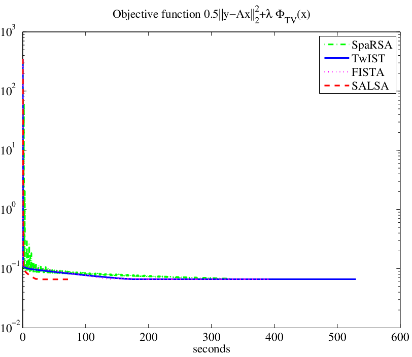
We consider the problem of reconstructing the Shepp-Logan phantom (shown in Figure 4) from a limited number of radial lines (22, in our experiments, as shown in Figure 4) of its 2D discrete Fourier transform. The projections are also corrupted with circular complex Gaussian noise, with variance . We use TV regularization (as described in Subsection IV-B), with the corresponding Moreau proximal mapping implemented by iterations of Chambolle’s algorithm [10].


Table V shows the CPU times, while Figure 5 plots the evolution of the objective function over time. Figure 4 shows the estimate obtained using SALSA (the others are, naturally, visually indistinguishable). Again, we may conclude that SALSA is considerably faster than the other three algorithms, while achieving comparable values of mean squared error of the reconstructed image.
| TwIST | SpARSA | FISTA | SALSA | |
|---|---|---|---|---|
| Iterations | 1002 | 1001 | 1000 | 53 |
| CPU time (seconds) | 529.297 | 328.688 | 390.75 | 76.5781 |
| MSE | 4.384e-7 | 6.033e-5 | 4.644e-7 | 5.817e-7 |
IV-D Image Inpainting
Finally, we consider an image inpainting problem, as explained in Section III-C. The original image is again the Cameraman, and the observation consists in loosing of its pixels, as shown in Figure 6. The observations are also corrupted with Gaussian noise (with an SNR of dB). The regularizer is again TV implemented by iterations of Chambolle’s algorithm.


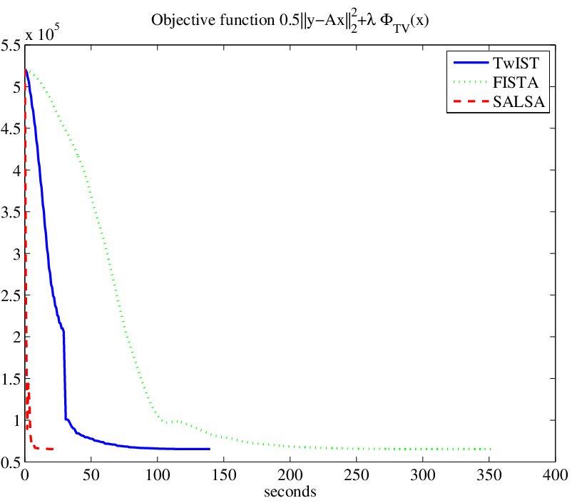
The image estimate obtained by SALSA is shown in Figure 6, with the original also shown for comparison. The estimates obtained using TwIST and FISTA were visually very similar. Table VI compares the performance of SALSA with that of TwIST and FISTA and Figure 7 shows the evolution of the objective function for each of the algorithms. Again, SALSA is considerably faster than the alternative algorithms.
| TwIST | FISTA | SALSA | |
| Iterations | 302 | 300 | 33 |
| CPU time (seconds) | 305 | 228 | 23 |
| MSE | 105 | 101 | 99.1 |
| ISNR (dB) | 18.4 | 18.5 | 18.6 |
V Conclusions
We have presented a new algorithm for solving the unconstrained optimization formulation of regularized image reconstruction/restoration. The approach, which can be used with different types of regularization (wavelet-based, total variation), is based on a variable splitting technique which yields an equivalent constrained problem. This constrained problem is then addressed using an augmented Lagrangian method, more specifically, the alternating direction method of multipliers (ADMM). The algorithm uses a regularized version of the Hessian of the data-fidelity term, which can be computed efficiently for several classes of problems. Experiments on a set of standard image recovery problems (deconvolution, MRI reconstruction, inpainting) have shown that the proposed algorithm (termed SALSA, for split augmented Lagrangian shrinkage algorithm) is faster than previous state-of-the-art methods. Current and future work involves using a similar approach to solve constrained formulations of the forms (3) and (4).
References
- [1] H. Andrews and B. Hunt. Digital Image Restoration, Prentice Hall, Englewood Cliffs, NJ, 1977.
- [2] O. Axelsson, Iterative Solution Methods, Cambridge University Press, New York, 1996.
- [3] M. Bazaraa, H. Sherali, and C. Shetty, Nonlinear Programming: Theory and Algorithms, John Wiley & Sons, New York, 1993.
- [4] A. Beck and M. Teboulle, “A fast iterative shrinkage-thresholding algorithm for linear inverse problems”, SIAM Journal on Imaging Sciences, vol. 2, pp. 183–202, 2009.
- [5] J. Bioucas-Dias and M. Figueiredo, “A new TwIST: two-step iterative shrinkage/thresholding algorithms for image restoration”, IEEE Transactions on Image Processing, vol. 16, no. 12, pp. 2992-3004, 2007.
- [6] J. Bioucas-Dias and M. Figueiredo, “An iterative algorithm for linear inverse problems with compound regularizers”, IEEE International Conference on Image Processing - ICIP’2008, San Diego, CA, USA, 2008.
- [7] E. Candès, L. Demanet, D. Donoho, and L. Ying, “Fast discrete curvelet transforms”, Multiscale Modelling and Simulation, vol. 5, pp. 861–899, 2005.
- [8] E. Candès, J. Romberg and T. Tao. “Stable signal recovery from incomplete and inaccurate information,” Communications on Pure and Applied Mathematics, vol. 59, pp. 1207–1233, 2005.
- [9] E. Candès, J. Romberg, and T. Tao. “Robust uncertainty principles: Exact signal reconstruction from highly incomplete frequency information,” IEEE Transactions on Information Theory, vol. 52, pp. 489–509, 2006.
- [10] A. Chambolle, “An algorithm for total variation minimization and applications,” J. Math. Imaging Vis., vol. 20, no. 1-2, pp. 89–97, 2004.
- [11] T. Chan, S. Esedoglu, F. Park, and A. Yip, “Recent developments in total variation image restoration”, in Handbook of Mathematical Models in Computer Vision, N. Paragios, Y. Chen, O. Faugeras (Editors), Springer Verlag, 2005.
- [12] P. Combettes and J.-C. Pesquet, “A Douglas-Rachford splitting approach to nonsmooth convex variational signal recovery”, IEEE Journal of Selected Topics in Signal Processing, vol. 1, pp. 564–574, 2007.
- [13] P. Combettes and V. Wajs, “Signal recovery by proximal forward-backward splitting,” SIAM Journal on Multiscale Modeling & Simulation, vol. 4, pp. 1168–1200, 2005.
- [14] R. Courant, “Variational methods for the solution of problems with equilibrium and vibration”, Bulletin of the American Mathematical Society, vol. 49, pp. 123, 1943.
- [15] I. Daubechies, M. De Friese, and C. De Mol. “An iterative thresholding algorithm for linear inverse problems with a sparsity constraint.” Communications in Pure and Applied Mathematics, vol. 57, pp. 1413–1457, 2004.
- [16] D. Donoho. “Compressed sensing,” IEEE Transactions on Information Theory, vol. 52, pp. 1289–1306, 2006.
- [17] J. Eckstein and D. Bertsekas, “On the DouglasRachford splitting method and the proximal point algorithm for maximal monotone operators”, Mathematical Programming, vol. 5, pp. 293-318, 1992.
- [18] M. Elad, B. Matalon, and M. Zibulevsky, “Image denoising with shrinkage and redundant representations”, Proceedings of the IEEE Computer Society Conference on Computer Vision and Pattern Recognition – CVPR’2006, New York, 2006.
- [19] M. Elad, P. Milanfar, and R. Rubinstein, “Analysis versus synthesis in signal priors”, Inverse Problems, vol. 23, pp. 947–968, 2007.
- [20] M. Figueiredo, J. Bioucas-Dias, and M. Afonso, “Fast frame-based image deconvolution using variable splitting and constrained optimization”, Proceedings of the IEEE Workshop on Statistical Signal Processing – SSP’2009, Cardiff, 2009.
- [21] M. Figueiredo, J. Bioucas-Dias, and R. Nowak, “Majorization-minimization algorithms for wavelet-based image restoration” IEEE Transactions on Image Processing, vol. 16, no. 12, pp. 2980–2991, 2007.
- [22] M. Figueiredo and R. Nowak. “An EM algorithm for wavelet-based image restoration.” IEEE Transactions on Image Processing, vol. 12, pp. 906–916, 2003.
- [23] M. Figueiredo and R. Nowak. “A bound optimization approach to wavelet-based image deconvolution”, Proceedings of the IEEE International Conference on Image Processing – ICIP’2005, Genoa, Italy, 2005.
- [24] M. Figueiredo, R. Nowak, S. Wright, “Gradient projection for sparse reconstruction: application to compressed sensing and other inverse problems,” IEEE Journal on Selected Topics in Signal Processing, vol. 1, pp. 586–598, 2007.
- [25] T. Goldstein and S. Osher, “The split Bregman algorithm for regularized problems”, Technical Report 08-29, Computational and Applied Mathematics, University of California, Los Angeles, 2008.
- [26] E. Esser, “Applications of Lagrangian-based alternating direction methods and connections to split-Bregman”, Technical Report 09-31, Computational and Applied Mathematics, University of California, Los Angeles, 2009.
- [27] T. Hale, W. Yin, Y. Zhang, “A fixed-point continuation method for -regularized minimization with applications to compressed sensing.” TR07-07, Department of Computational and Applied Mathematics, Rice University, 2007.
- [28] M. Hestenes, “Multiplier and gradient methods”, Journal of Optimization Theory and Applications, vol. 4, pp. 303–320, 1969.
- [29] D. Hunter and K. Lange. “A tutorial on MM algorithms.” The American Statistician, vol. 58, pp. 30–37, 2004.
- [30] A. Iusem, “Augmented Lagrangian methods and proximal point methods for convex optimization”, Investigación Operativa, vol. 8, pp. 11–49, 1999.
- [31] N. Kingsbury, “Complex wavelets for shift invariant analysis and filtering of signals”, Journal of Applied and Computational Harmonic Analysis, vol. 10, pp. 234-253, 2001.
- [32] M. Lang, H. Guo, J. Odegard, C. Burrus and R. Wells. “Noise reduction using an undecimated discrete wavelet transform,” IEEE Signal Processing Letters, vol. 3, pp. 10–12, 1996.
- [33] M. Lustig, D. Donoho, and J. Pauly, “Sparse MRI: the application of compressed sensing for rapid MR imaging,” Magnetic Resonance in Medicine, vol. 58, pp. 1182–1195, 2007.
- [34] S. Mallat. A Wavelet Tour of Signal Processing. Academic Press, San Diego, CA, 1998.
- [35] Y. Nesterov, “A method for solving the convex programming problem with convergence rate ”, Soviet Math. Doklady, vol. 269, pp. 543-547, 1983 (in Russian).
- [36] Y. Nesterov, Introductory Lectures on Optimization, Kluwer Academic Publishers, Dordrecht, The Netherlands, 2004.
- [37] J. Nocedal, S. J. Wright. Numerical Optimization, 2nd Edition, Springer, 2006.
- [38] M. Powell, “A method for nonlinear constraints in minimization problems”, in Optimization, R. Fletcher (Editor), pp. 283-298, Academic Press, New York, 1969.
- [39] R. T. Rockafellar, Convex Analysis, Princeton University Press, Princeton, NJ, 1970.
- [40] L. Rudin, S. Osher, and E. Fatemi, Nonlinear total variation based noise removal algorithms, Physica D, vol. 60, pp. 259–268, 1992.
- [41] I. Selesnick, “Hilbert transform pairs of wavelet bases”, IEEE Signal Processing Letters, vol. 8, pp. 170-173, 2001.
- [42] S. Setzer, “Split Bregman algorithm, Douglas-Rachford splitting, and frame shrinkage”, Proceedings of the Second International Conference on Scale Space Methods and Variational Methods in Computer Vision, Springer, 2009.
- [43] Y. Wang, J. Yang, W. Yin, and Y. Zhang, “A new alternating minimization algorithm for total variation image reconstruction”, SIAM Journal on Imaging Sciences, vol. 1, pp. 248–272, 2008.
- [44] S. Wright, R. Nowak, M. Figueiredo, “Sparse reconstruction by separable approximation, Proceedings of the IEEE International Conference on Acoustics, Speech, and Signal Processing ICASSP2008, Las Vegas, NV, USA, 2008.
- [45] S. Wright, R. Nowak, M. Figueiredo, “Sparse reconstruction by separable approximation, IEEE Transactions on Signal Processing, vol. 57, pp. 2479–2493, 2009.
- [46] W. Yin, S. Osher, D. Goldfarb, and J. Darbon, “Bregman iterative algorithms for minimization with applications to compressed sensing”, SIAM Journal on Imaging Science, vol. 1, pp. 143–168, 2008.