Physical properties of the 0.94-day period transiting planetary system WASP-18
Abstract
We present high-precision photometry of five consecutive transits of WASP-18, an extrasolar planetary system with one of the shortest orbital periods known. Through the use of telescope defocussing we achieve a photometric precision of 0.47–0.83 mmag per observation over complete transit events. The data are analysed using the jktebop code and three different sets of stellar evolutionary models. We find the mass and radius of the planet to be and (statistical and systematic errors) respectively. The systematic errors in the orbital separation and the stellar and planetary masses, arising from the use of theoretical predictions, are of a similar size to the statistical errors and set a limit on our understanding of the WASP-18 system. We point out that seven of the nine known massive transiting planets () have eccentric orbits, whereas significant orbital eccentricity has been detected for only four of the 46 less massive planets. This may indicate that there are two different populations of transiting planets, but could also be explained by observational biases. Further radial velocity observations of low-mass planets will make it possible to choose between these two scenarios.
I. Introduction
The recent discovery of the transiting extrasolar planetary system WASP-18 [16, hereafter H09] lights the way towards understanding the tidal interactions between giant planets and their parent stars. WASP-18 b is one of the shortest-period ( d) and most massive () extrasolar planets known. These properties make it an unparallelled indicator of the tidal dissipation parameters [15] for the star and the planet [17]. A value similar to that observed for Solar system bodies (–; Peale 24) would cause the orbital period of WASP-18 to decrease at a sufficient rate for the effect to be observable within ten years (H09).
In this work we present high-precision follow-up photometry of WASP-18, obtained using telescope-defocussing techniques [36, 37] which give a scatter of only 0.47 to 0.83 mmag per observation. These are analysed to yield improved physical properties of the WASP-18 system, with careful attention paid to statistical and systematic errors. The quality of the light curve is a critical factor in measurement of the physical properties of transiting planets [29]. In the case of WASP-18 the systematic errors arising from the use of theoretical stellar models are also important, and are a limiting factor in the understanding of this system.
II. Observations and data reduction
| Date | Start time (UT) | End time (UT) | Exposure time (s) | Filter | Airmass | Moon | Distance (∘) | Scatter (mmag) | |
|---|---|---|---|---|---|---|---|---|---|
| 2009 09 07 | 06:41 | 10:05 | 93 | 80.0 | 1.05 1.27 | 0.860 | 61.9 | 0.83 | |
| 2009 09 08 | 05:00 | 10:04 | 140 | 80.0 | 1.15 1.04 1.28 | 0.784 | 67.1 | 0.68 | |
| 2009 09 09 | 03:55 | 10:00 | 169 | 80.0 | 1.31 1.04 1.27 | 0.696 | 73.3 | 0.51 | |
| 2009 09 10 | 03:25 | 08:29 | 141 | 80.0 | 1.41 1.04 1.10 | 0.597 | 80.2 | 0.56 | |
| 2009 09 11 | 04:07 | 07:12 | 86 | 80.0 | 1.25 1.04 | 0.492 | 87.6 | 0.47 |
We observed five consecutive transits of WASP-18 on the nights of 2009 September 7–11, using the 1.54 m Danish Telescope at ESO La Silla with the focal-reducing imager DFOSC. The plate scale of this setup is 0.39′′ pixel-1. The CCD was windowed down to an area of 12′8′ in order to decrease the readout time to 51 s. This window was chosen to include WASP-18 (HD 10069, spectral type F6 V, , ) and a good comparison star (HD 10179, spectral type F3 V, , ).
A Johnson filter and exposure times of 80 s were used (instead of our usual Cousins and 120 s), to obtain lower count rates from the target and comparison stars. We defocussed the telescope to a point spread function (PSF) diameter of 90 pixels (35′′), to limit the peak counts to 45 000 per pixel for WASP-18 and also lower the flat-fielding noise. This focus setting was used for all observations and the pointing of the telescope was maintained using autoguiding. An observing log is given in Table 1.
We took several images with the telescope properly focussed in order to check that there were no nearby stars contaminating the PSF of WASP-18. There are five detectable objects nearby, but all are at least 100 pixels distant. The brightest is 6.75 mag fainter than WASP-18 and the other four are more than 9.5 mag fainter. We conclude that the PSF of WASP-18 is not contaminated by any star detectable with our equipment.
Data reduction was performed in the same way as in Southworth et al. [36], Southworth et al. [37]. In short, we run a reduction pipeline written in idl11 1 The acronym idl stands for Interactive Data Language and is a trademark of ITT Visual Information Solutions. For further details see http://www.ittvis.com/ProductServices/IDL.aspx. which uses an implementation of the daophot package [38] to perform aperture photometry. For each night’s data the apertures were placed interactively and their positions fixed for each CCD image. We found that the most precise photometry was obtained using an object aperture of radius 60 pixels and a sky annulus of radius 85–110 pixels. The choice of aperture sizes (within reason) excludes flux from the nearby faint stars, and has a negligible effect on the resulting photometry.
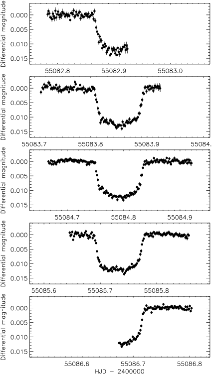
We calculated differential magnitudes for WASP-18 using an ensemble of four comparison stars, of which HD 10179 is by far the brightest. The light curve for each night was normalised to zero differential magnitude by fitting a straight line to the observations taken outside transit, whilst simultaneously optimising the weights of the four comparison stars. We have applied bias and flat-field corrections to the images, but find that this does not have a significant effect on the photometry. The individual light curves are shown in Fig. 1, and the full 629 datapoints are given in Table 2. The scatter in the final light curves varies from 0.47 to 0.83 mmag per point, and is higher for data taken when the moon was bright (Table 1).
| Midpoint of | Relative | Error in |
|---|---|---|
| observation (BJD) | magnitude | magnitude |
| 55082.783033 | 0.000200 | 0.000788 |
| 55082.784491 | 0.001340 | 0.000790 |
| 55082.786030 | 0.000495 | 0.000786 |
| 55082.787570 | 0.000825 | 0.000786 |
| 55082.789109 | 0.000989 | 0.000804 |
| 55082.790649 | 0.001469 | 0.000880 |
| 55082.792188 | 0.000431 | 0.000965 |
| 55082.793727 | 0.000483 | 0.001159 |
| 55082.795267 | 0.001142 | 0.001067 |
| 55082.796806 | 0.001431 | 0.001156 |
III. Light curve analysis
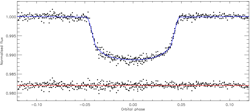
The light curves of WASP-18 were analysed with the jktebop22 2 jktebop is written in fortran77 and the source code is available at http://www.astro.keele.ac.uk/jkt/ code [30, 31], using the approach discussed in detail by Southworth [28]. jktebop approximates the two components of WASP-18 using biaxial spheroids whose shapes are governed by the mass ratio; we adopt the value 0.008 but find that large changes in this number have a negligible effect on the results.
WASP-18 b has a slightly eccentric orbit, which should be taken into account as it has a small effect on the shape of the transit. However, for transit light curves the effect is in general too subtle to include it as a fitted parameter [21]. We could fix eccentricity, , and periastron longitude, , to the values obtained from the velocity variation of the parent star (H09), but this would neglect their measurement uncertainties. We have therefore modified jktebop to allow the inclusion of and as fitted parameters constrained by the known values and uncertainties. In practise we use and , as these two parameters are only weakly correlated with each other. In the current case the uncertainties in the and values have a very minor effect on our results.
We have incorporated the H09 photometry of WASP-18 in order to obtain the most precise ephemeris. This was done by including the reference transit epoch from H09 as an observed quantity, and then fitting for transit epoch and orbital period directly [35, see]. We chose a new transit epoch which is close to the midpoint of our own observations, so is essentially based on just the data presented in this work. The final eclipse ephemeris is
where is the transit midpoint, is the number of orbital cycles after the reference epoch, and quantities in parentheses denote the uncertainty in the final digit of the preceding number.
| Linear LD law | Quadratic LD law | Square-root LD law | Logarithmic LD law | Cubic LD law | ||||||
| All LD coefficients fixed | ||||||||||
| 0.3094 | 0.0075 | 0.3034 | 0.0074 | 0.3060 | 0.0077 | 0.3069 | 0.0075 | 0.3176 | 0.0068 | |
| 0.09704 | 0.00075 | 0.09636 | 0.00057 | 0.09682 | 0.00069 | 0.09712 | 0.00062 | 0.09912 | 0.00048 | |
| (deg.) | 84.68 | 1.33 | 85.96 | 1.70 | 85.31 | 1.51 | 85.05 | 1.35 | 83.05 | 0.90 |
| 0.60 fixed | 0.40 fixed | 0.20 fixed | 0.70 fixed | 0.40 fixed | ||||||
| 0.30 fixed | 0.60 fixed | 0.25 fixed | 0.15 fixed | |||||||
| 0.94145182 | 0.00000040 | 0.94145181 | 0.00000041 | 0.94145182 | 0.00000044 | 0.94145181 | 0.00000045 | 0.94145181 | 0.00000043 | |
| 84.792935 | 0.000090 | 84.792929 | 0.000085 | 84.792932 | 0.000084 | 84.792931 | 0.000084 | 84.792924 | 0.000085 | |
| 0.2821 | 0.0067 | 0.2767 | 0.0066 | 0.2790 | 0.0069 | 0.2798 | 0.0067 | 0.2890 | 0.0060 | |
| 0.02737 | 0.00085 | 0.02667 | 0.00078 | 0.02701 | 0.00085 | 0.02717 | 0.00081 | 0.02864 | 0.00072 | |
| (mag) | 0.6406 | 0.6358 | 0.6356 | 0.6355 | 0.6408 | |||||
| 1.0194 | 1.0048 | 1.0031 | 1.0034 | 1.0247 | ||||||
| Fitting for the linear LD coefficient and fixing the nonlinear LD coefficient | ||||||||||
| 0.3106 | 0.0070 | 0.3053 | 0.0082 | 0.3073 | 0.0080 | 0.3066 | 0.0076 | 0.3071 | 0.0079 | |
| 0.09813 | 0.00070 | 0.09672 | 0.00087 | 0.09720 | 0.00082 | 0.09702 | 0.00081 | 0.09726 | 0.00086 | |
| (deg.) | 84.2 | 1.1 | 85.5 | 1.8 | 85.0 | 1.5 | 85.1 | 1.5 | 85.0 | 1.5 |
| 0.527 | 0.023 | 0.384 | 0.029 | 0.180 | 0.024 | 0.705 | 0.025 | 0.495 | 0.025 | |
| 0.30 fixed | 0.60 fixed | 0.25 fixed | 0.15 fixed | |||||||
| 0.94145182 | 0.00000043 | 0.94145181 | 0.00000041 | 0.94145182 | 0.00000042 | 0.94145181 | 0.00000042 | 0.94145182 | 0.00000039 | |
| 84.792931 | 0.000080 | 84.792930 | 0.000089 | 84.792931 | 0.000086 | 84.792931 | 0.000081 | 84.792932 | 0.000084 | |
| 0.2829 | 0.0062 | 0.2784 | 0.0072 | 0.2801 | 0.0071 | 0.2795 | 0.0068 | 0.2799 | 0.0070 | |
| 0.02776 | 0.00078 | 0.02692 | 0.00094 | 0.02722 | 0.00090 | 0.02711 | 0.00086 | 0.02722 | 0.00088 | |
| (mag) | 0.6357 | 0.6356 | 0.6352 | 0.6355 | 0.6350 | |||||
| 1.0048 | 1.0061 | 1.0037 | 1.0049 | 1.0031 | ||||||
| Fitting for the linear LD coefficient and perturbing the nonlinear LD coefficient | ||||||||||
| 0.3106 | 0.0066 | 0.3053 | 0.0084 | 0.3073 | 0.0079 | 0.3066 | 0.0081 | 0.3071 | 0.0079 | |
| 0.09813 | 0.00069 | 0.09672 | 0.00092 | 0.09720 | 0.00081 | 0.09702 | 0.00086 | 0.09726 | 0.00083 | |
| (deg.) | 84.2 | 1.0 | 85.5 | 1.8 | 85.0 | 1.5 | 85.1 | 1.6 | 85.0 | 1.5 |
| 0.527 | 0.022 | 0.384 | 0.039 | 0.180 | 0.042 | 0.705 | 0.053 | 0.495 | 0.028 | |
| 0.30 perturbed | 0.60 perturbed | 0.25 perturbed | 0.15 perturbed | |||||||
| 0.94145182 | 0.00000042 | 0.94145181 | 0.00000043 | 0.94145182 | 0.00000043 | 0.94145181 | 0.00000043 | 0.94145182 | 0.00000043 | |
| 84.792931 | 0.000086 | 84.792930 | 0.000085 | 84.792931 | 0.000080 | 84.792931 | 0.000084 | 84.792932 | 0.000084 | |
| 0.2829 | 0.0059 | 0.2784 | 0.0075 | 0.2801 | 0.0070 | 0.2795 | 0.0072 | 0.2799 | 0.0070 | |
| 0.02776 | 0.00076 | 0.02692 | 0.00095 | 0.02722 | 0.00086 | 0.02711 | 0.00090 | 0.02722 | 0.00091 | |
| (mag) | 0.6357 | 0.6356 | 0.6352 | 0.6355 | 0.6350 | |||||
| 1.0048 | 1.0061 | 1.0037 | 1.0049 | 1.0031 | ||||||
| Fitting for both LD coefficients | ||||||||||
| 0.3106 | 0.0070 | 0.3064 | 0.0086 | 0.3068 | 0.0083 | 0.3063 | 0.0083 | 0.3071 | 0.0081 | |
| 0.09813 | 0.00070 | 0.09740 | 0.00117 | 0.09721 | 0.00144 | 0.09737 | 0.00128 | 0.09721 | 0.00140 | |
| (deg.) | 84.2 | 1.1 | 85.0 | 1.7 | 85.0 | 1.9 | 85.0 | 1.7 | 85.0 | 1.8 |
| 0.527 | 0.022 | 0.473 | 0.087 | 0.213 | 0.433 | 0.617 | 0.175 | 0.492 | 0.045 | |
| 0.11 | 0.18 | 0.54 | 0.77 | 0.12 | 0.24 | 0.16 | 0.20 | |||
| 0.94145182 | 0.00000041 | 0.94145181 | 0.00000044 | 0.94145181 | 0.00000043 | 0.94145182 | 0.00000044 | 0.94145181 | 0.00000041 | |
| 84.792931 | 0.000086 | 84.792932 | 0.000089 | 84.792931 | 0.000084 | 84.792932 | 0.000088 | 84.792931 | 0.000084 | |
| 0.2829 | 0.0062 | 0.2792 | 0.0076 | 0.2796 | 0.0072 | 0.2792 | 0.0073 | 0.2799 | 0.0071 | |
| 0.02776 | 0.00078 | 0.02719 | 0.00103 | 0.02718 | 0.00108 | 0.02718 | 0.00103 | 0.02721 | 0.00105 | |
| (mag) | 0.6357 | 0.6353 | 0.6352 | 0.6354 | 0.6350 | |||||
| 1.0048 | 1.0055 | 1.0053 | 1.0057 | 1.0047 | ||||||
The limb darkening (LD) of WASP 18 A was accounted for using five different parametric laws [28, see]. Theoretical LD coefficients were obtained by bilinear interpolation, to the known effective temperature () and surface gravity of the parent star, in the tables of Van Hamme [39], Claret [5], Claret [6] and Claret & Hauschildt [11]. We obtained solutions with the LD coefficients fixed at the theoretical values, with the linear coefficient fitted for and the nonlinear coefficient fixed (and optionally perturbed by 0.05 on a flat distribution in the error analyses), and with both LD coefficients included as fitted parameters. The full set of solutions is given in Table 3.
The uncertainties of the light curve parameters were assessed using Monte Carlo simulations [32, 34]. The importance of red noise was checked using a residual-permutation approach, and found to be minor. The solutions with LD coefficients fixed to theoretical values are poorer than those where one or both LD coefficients are fitted parameters. We adopt the mean of the solutions with non-linear LD and both LD coefficients fitted, as these are the most internally consistent. The final uncertainties come from Monte Carlo solutions but include contributions from the residual-permutation analyses and the (minor) variation between the solutions with different LD laws. We find the fractional radius33 3 Fractional radius is the radius of a component of a binary system expressed as a fraction of the orbital semimajor axis. The utility of this quantity is that it is measureable from light curve data alone. of the star and planet to be and , respectively, and the orbital inclination to be .
IV. The physical properties of WASP-18
| Cambridge models | Y2 models | Claret models | Final result (this work) | Hellier et al. [16] | ||||||||
| Orbital separation | (AU) | 0.02022 | 0.00022 | 0.02043 | 0.00028 | 0.02047 | 0.00027 | 0.02047 | 0.00028 | 0.00025 | 0.02026 | 0.00068 |
| Stellar mass | () | 1.235 | 0.039 | 1.274 | 0.052 | 1.281 | 0.050 | 1.281 | 0.052 | 0.046 | 1.25 | 0.13 |
| Stellar radius | () | 1.215 | 0.048 | 1.227 | 0.043 | 1.230 | 0.042 | 1.230 | 0.045 | 0.015 | ||
| Stellar | [cgs] | 4.361 | 0.022 | 4.365 | 0.026 | 4.366 | 0.026 | 4.366 | 0.026 | 0.005 | ||
| Stellar density | () | 0.689 | 0.062 | 0.689 | 0.062 | 0.689 | 0.062 | 0.689 | 0.062 | 0.000 | ||
| Planetary mass | () | 10.18 | 0.22 | 10.39 | 0.30 | 10.43 | 0.28 | 10.43 | 0.30 | 0.24 | 10.30 | 0.69 |
| Planetary radius | () | 1.151 | 0.052 | 1.163 | 0.055 | 1.165 | 0.054 | 1.165 | 0.055 | 0.014 | ||
| Planet surface gravity | ( m s-2) | 191 | 17 | 191 | 17 | 191 | 17 | 191 | 17 | |||
| Planetary density | () | 6.68 | 0.89 | 6.61 | 0.89 | 6.60 | 0.88 | 6.60 | 0.90 | 0.08 | ||
| Stellar age | (Gyr) | 0.0 – 0.6 | 0.0 – 2.1 | 0.0 – 2.0 | 0.5 – 1.5 | |||||||
The physical properties of a transiting planetary system cannot in general be calculated purely from observed quantities. The most common way to overcome this difficulty is to impose predictions from theoretical stellar evolutionary models onto the parent star. We have used tabulated predictions from three sources: Claret [7, 8, 9, 10], Y2 [12] and Cambridge [25, 13]. This allows the assessment of the systematic errors caused by using stellar theory.
We began with the parameters measured from the light curve and the observed velocity amplitude of the parent star, m s-1 (H09). These were augmented by an estimate of the velocity amplitude of the planet, , to calculate preliminary physical properties of the system. We then interpolated within one of the grids of theoretical predictions to find the expected radius and of the star for the preliminary mass and the measured metal abundance (; H09). was then iteratively refined to minimise the difference between the model-predicted radius and , and the calculated radius and measured ( K; H09). This was done for a range of ages for the star, and the best overall fit retained as the optimal solution. Finally, the above process was repeated whilst varying every input parameter by its uncertainty to build up a complete error budget for each output parameter [33]. A detailed description of this process can be found in Southworth [29].
Table 4 shows the results of these analyses. The physical properties calculated using the Claret and Y2 sets of stellar models are in excellent agreement, but those from the Cambridge models are slightly discrepant. This causes systematic errors of 4% in the stellar mass and 2% in the planetary mass, both of similar size to the corresponding statistical errors. The quality of our results is therefore limited by our theoretical understanding of the parent star. Our final results are in good agreement with those of H09 (Table 4), but incorporate a more comprehensive set of uncertainties.
These results give the equilibrium temperature of the planet to be one of the highest for the known planets:
where is the Bond albedo and is the heat redistribution factor. This equilibrium temperature, and the closeness to its parent star, make WASP-18 b a good target for the detection of thermal emission and reflected light.
V. Conclusions
We have presented high-quality observations of five consecutive transits by the newly-discovered planet WASP-18 b, which has one of the shortest orbital periods of all known transiting extrasolar planetary systems (TEPs). Our defocussed-photometry approach yielded scatters of between 0.47 and 0.83 mmag per point in the final light curves. These data were analysed using the jktebop code, which was modified to include the spectroscopically derived orbital eccentricity in a statistically correct way. The light curve parameters were then combined with the predictions of theoretical stellar evolutionary models to determine the physical properties of the planet and its host star.
A significant source of uncertainty in our results stems from the use of theoretical models to constrain the physical properties of the star. Further uncertainty comes from observed and , for which improved values are warranted. However, the systematic error from the use of stellar theory is an important uncertainty in the masses of the star and planet. This is due to our fundamentally incomplete understanding of the structure and evolution of low-mass stars. As with many other transiting systems (e.g. WASP-4; Southworth et al. 37), our understanding of the planet is limited by our lack of understanding of the parent star.
We confirm and refine the physical properties of WASP 18 found by H09. WASP-18 b is a very massive planet in an extremely short-period and eccentric orbit, which is a clear indicator that the tidal effects in planetary systems are weaker than expected (see H09). Long-term follow-up studies of WASP-18 will add progressively stricter constraints on the orbital decay of the planet and thus the strength of these tidal effects.
We now split the full sample of known (i.e. published) TEPS into two classes according to planetary mass. The mass distribution of transiting planets shows a dearth of objects with masses in the interval 2.0–3.1. There are nine planets more massive than this and 46 less massive. Seven of the nine high-mass TEPs have eccentric orbits (HAT-P-2, Bakos et al. 2; HD 17156, Barbieri et al. 3; HD 80606, Laughlin et al. 22; WASP-10, Christian et al. 4; WASP-14, Joshi et al. 20; WASP-18; XO-3, Johns-Krull et al. 18), and the existing radial velocity observations of the remaining two cannot rule out an eccentricity of or lower (CoRoT-Exo-2, Alonso et al. 1; OGLE-TR-L9, Snellen et al. 27). By comparison, only four of the 46 low-mass TEPs have a significant [23] orbital eccentricity measurement.
These numbers imply that the more massive TEPs are a different population to the less massive ones; Fisher’s exact test [14] returns a probability lower than of the null hypothesis (although this does not account for our freedom to choose the dividing line between the two classes). This indicates that the two types of TEPs have a different internal structure, formation mechanism, or evolution, a suggestion which is supported by observations of misalignment between the spin and orbital axes of TEPs [19].
There is, however, a bias at work here. The more massive TEPs cause a larger radial velocity signal in their parent star (), so a given set of radial velocity measurements can detect smaller eccentricities [26, see also]. The eccentricity of the WASP-18 system is in fact below the detection limit of existing observations of most TEPs. We therefore advocate the acquisition of additional velocity data for the known low-mass TEPs, in order to equalise the eccentricity detection limits between the two classes of TEPs. These observations would allow acceptance or rejection of the hypothesis that more massive TEPs represent a fundamentally different planet population to their lower-mass brethren.
References
- [1] Alonso, R., et al., 2008, A&A, 482, L21
- [2] Bakos, G. Á., et al., 2007, ApJ, 670, 826
- [3] Barbieri, M., et al., 2007, A&A, 476, L13
- [4] Christian, D. J., et al., 2009, MNRAS, 392, 1585
- [5] Claret, A., 2000, A&A, 363, 1081
- [6] Claret, A., 2004a, A&A, 428, 1001
- [7] Claret, A., 2004b, A&A, 424, 919
- [8] Claret, A., 2005, A&A, 440, 647
- [9] Claret, A., 2006, A&A, 453, 769
- [10] Claret, A., 2007, A&A, 467, 1389
- [11] Claret, A., Hauschildt, P. H., 2003, A&A, 412, 241
- [12] Demarque, P., Woo, J.-H., Kim, Y.-C., Yi, S. K., 2004, ApJS, 155, 667
- [13] Eldridge, J. J., Tout, C. A., 2004, MNRAS, 353, 87
- [14] Fisher, R. A., 1922, Journal of the Royal Statistical Society, 85, 87
- [15] Goldreich, P., Soter, S., 1966, Icarus, 5, 375
- [16] Hellier, C., et al., 2009, Nature, 460, 1098
- [17] Jackson, B., Barnes, R., Greenberg, R., 2009, ApJ, 698, 1357
- [18] Johns-Krull, C. M., et al., 2008, ApJ, 677, 657
- [19] Johnson, J. A., Winn, J. N., Albrecht, S., Howard, A. W., Marcy, G. W., Gazak, J. Z., 2009, PASP, 121, 1104
- [20] Joshi, Y. C., et al., 2009, MNRAS, 392, 1532
- [21] Kipping, D. M., 2008, MNRAS, 389, 1383
- [22] Laughlin, G., Deming, D., Langton, J., Kasen, D., Vogt, S., Butler, P., Rivera, E., Meschiari, S., 2009, Nature, 457, 562
- [23] Lucy, L. B., Sweeney, M. A., 1971, AJ, 76, 544
- [24] Peale, S. J., 1999, ARA&A, 37, 533
- [25] Pols, O. R., Schroder, K.-P., Hurley, J. R., Tout, C. A., Eggleton, P. P., 1998, MNRAS, 298, 525
- [26] Shen, Y., Turner, E. L., 2008, ApJ, 685, 553
- [27] Snellen, I. A. G., et al., 2009, A&A, 497, 545
- [28] Southworth, J., 2008, MNRAS, 386, 1644
- [29] Southworth, J., 2009, MNRAS, 394, 272
- [30] Southworth, J., Maxted, P. F. L., Smalley, B., 2004a, MNRAS, 349, 547
- [31] Southworth, J., Maxted, P. F. L., Smalley, B., 2004b, MNRAS, 351, 1277
- [32] Southworth, J., Zucker, S., Maxted, P. F. L., Smalley, B., 2004c, MNRAS, 355, 986
- [33] Southworth, J., Maxted, P. F. L., Smalley, B., 2005a, A&A, 429, 645
- [34] Southworth, J., Smalley, B., Maxted, P. F. L., Claret, A., Etzel, P. B., 2005b, MNRAS, 363, 529
- [35] Southworth, J., Bruntt, H., Buzasi, D. L., 2007, A&A, 467, 1215
- [36] Southworth, J., et al., 2009a, MNRAS, 396, 1023
- [37] Southworth, J., et al., 2009b, MNRAS, in press (preprint arXiv:0907:3356)
- [38] Stetson, P. B., 1987, PASP, 99, 191
- [39] Van Hamme, W., 1993, AJ, 106, 2096