Determining the Anisotropic Exchange Coupling of CrO2 via First-Principles Density Functional Theory Calculations
Abstract
We report a study of the anisotropic exchange interactions in bulk CrO2 calculated from first principles within density functional theory.[8] We determine the exchange coupling energies, using both the experimental lattice parameters and those obtained within DFT, within a modified Heisenberg model Hamiltonian in two ways. We employ a supercell method in which certain spins within a cell are rotated and the energy dependence is calculated and a spin-spiral method that modifies the periodic boundary conditions of the problem to allow for an overall rotation of the spins between unit cells. Using the results from each of these methods, we calculate the spin-wave stiffness constant from the exchange energies using the magnon dispersion relation. We employ a Monte Carlo method to determine the DFT-predicted Curie temperature from these calculated energies and compare with accepted values. Finally, we offer an evaluation of the accuracy of the DFT-based methods and suggest implications of the competing ferro- and antiferromagnetic interactions.eting ferro- and antiferromagnetic interactions.
I Introduction
CrO2 is one of only a few known ferromagnetic oxides and is predicted to be a half-metal by first-principles calculations.[1] In fact, it is the only material which has been experimentally shown to be a ferromagnetic “half-metal,”[2, 3] a material that is a metal for one spin channel and an insulator for the other. CrO2 crystallizes in the rutile crystal structure (Figure 1), as do TiO2, VO2, MnO2, RuO2, and SnO2. The existence of isostructural oxides with a variety of different electronic and magnetic properties makes the rutile system interesting for theoretical investigations of spintronics because one can envisage the growth of layered devices with the same crystal structure throughout. Since CrO2 offers such special opportunities for understanding oxide spintronics, it is important to establish how well our standard electronic structure tools work in dealing with the electronic and magnetic structure of this material. It is well known that they encounter difficulties in dealing with many transition metal oxides, including the very similar oxide VO2, which DFT[8] also predicts to be a half-metal at 0K, [4] but is observed to be an insulator. An additional motivation for understanding exchange interactions in CrO2 is the fact that its Curie temperature ( K)[5, 6] is sufficiently close to room temperature that its magnetic properties are significantly degraded at room temperature, hindering potential spintronics applications. A better understanding may point the way to improvement.
In this work, we investigated the magnetic structure of CrO2 by considering three near neighbor Cr-Cr exchange interactions: the interaction between corner and body center atoms mediated through a single oxygen atom, the interaction between a Cr and the Cr directly “above” it in the (001) direction, and the interaction between a Cr and its neighbor in the (100) direction. The interactions were calculated by rotating the moments of one or more of the Cr ions while constraining the others to remain parallel. We then fit the resulting energy vs. angle data to the Heisenberg model and extracted exchange energy parameters with a least-squares method. We also calculated the exchange interactions using a “spin-spiral” technique, in which a relative angular displacement was imposed upon Cr moments in adjacent cells. Similar results were obtained with both approaches. The calculated K exchange interactions were subsequently used to determine the magnetization as a function of temperature via low-T spin-wave dispersion and a Monte-Carlo method.
II Electronic Structure of CrO2 Within Density Functional Theory
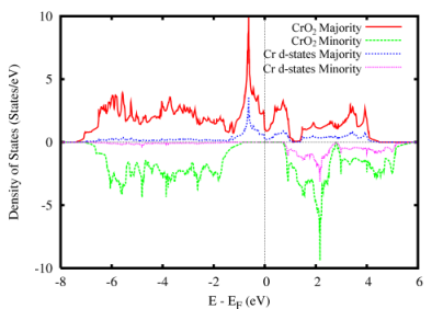
In the following, the electronic structure and density of states of CrO2 were calculated using density functional theory[8] (DFT) and the generalized gradient approximation[9] (GGA) using GGA-relaxed lattice parameters (see Table 2). Our calculated density of states is similar to previous calculations.[1, 10] For a detailed discussion of the electronic structure of the rutiles, we refer the reader to the work of Sorantin and Schwarz.[10] Additionally, the lattice structure is presented in Figure 1.

It is straightforward to show that if we treat this system in a tight-binding approximation in which the TM atoms only interact directly with the oxygen atoms (i.e. hopping matrix elements only connect nearest neighbors), there will be an energy gap separating the oxygen -states and the TM -states. The gap extends from the O- onsite energy to the TM- onsite energy. This gap is apparent in TiO2, for which the oxygen -states are filled and the Ti -states are empty (Fig. 2). When an energy gap occurs at the Fermi energy, it contributes significantly to reducing the energy of the structure, because all occupied states are pushed down in energy, while all unoccupied states are pushed up. In CrO2, there are two additional electrons per TM atom compared to TiO2, so some of the -states above the gap must be occupied.
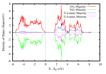
Comparing these the energies of the possible magnetic configurations (FM, AF, or nonmagnetic) using total-energy GGA DFT calculations (with GGA-relaxed lattice parameters), it is not surprising that we find that the ferromagnetic state has the lowest energy (with the DOS seen in Figure 3), the nonmagnetic state the highest (1.02 eV above ferromagnetic) with the anti-ferromagnetic intermediate between the two (0.30 eV above ferromagnetic). Thus, the tendency to form a moment in CrO2 is very strong, and the energy associated with the ferromagnetic alignment of moments based on this initial test is moderately large within DFT. It should be recognized that other more complicated spin arrangements (e.g. different antiferromagnetic states) may have lower energy than the simple one calculated here.
III Exchange Interactions in CrO2
In order to investigate interatomic exchange interactions in CrO2 in more detail, we have calculated the near-neighbor exchange interactions along the (100), (001), and (111) directions by rotating moments within specially-constructed supercells. We fit the resulting relationship between the energy of the system and the angle of rotation to the Heisenberg model
| (1) |
where is the spin moment, is the electron spin -factor, is the spin number, and is the Bohr magneton. To make contact with the standard Heisenberg model, we can pull the magnitude of the spin moment () into the value of and treat the spins as unit vectors.
In addition to this supercell approach, we have taken advantage of a recently developed feature in the Vienna Ab-initio Simulation Package[7] (VASP) to calculate a so-called helimagnetic state in which the moment in the magnetic layer is canted by an angle with respect to the layer. In so doing, we are able to calculate several orders of of the form
| (2) |
via Fourier analysis. The relationship between the and the will be made explicit in Section III.2.
III.1 Near Neighbor Exchange Using Supercells
All of the calculations in this study were performed within DFT[8] in the GGA[9] and in the local (spin) density approximation with onsite Coulomb interactions (LSDA+U)[11] using the Dudarev method,[12] for which we use = 2.1 eV, in agreement with the and values seen in other works.[13] We perform all calculations using the VASP software[7] and pseudopotentials generated by Kresse et al.[14]. To calculate the near-neighbor exchange interactions, we created a supercell containing two rutile unit cells (using both experimental and DFT-relaxed lattice parameters), stacked in either the (100) (Fig. 4) or (001) (Fig. 5) direction as appropriate. In all of the following calculations, we use an energy cut-off of 500 eV. For cells stacked along the (100) direction, we use a Monkhorst-Pack[15] grid of k-points, a grid for supercells stacked along (001), and a grid for the 6-atom cell used in the spin-spiral calculations. We also make use of the spin interpolation method of Vosko-Wilk-Nusair.[16] Each of the 12-atom supercells has four Cr ions, whose magnetic moments we can individually constrain within the calculation. We chose three distinct magnetic configurations designed to probe the exchange coefficients. In the first configuration, we rotated the moment of a corner Cr atom and held all other moments fixed using the constraining field method in VASP. In the second, we rotated the two Cr moments in the centers of their respective unit cells, and in the third we rotated a corner atom and its nearest center atom. A summary of the configurations can be found in Table 1.


| Cr1 | Cr2 | Cr3 | Cr4 | |
|---|---|---|---|---|
| Case 1 | fixed | rotated | fixed | fixed |
| Case 2 | rotated | rotated | fixed | fixed |
| Case 3 | rotated | fixed | rotated | fixed |
To ensure that we can accurately apply our modified Heisenberg model to these systems, we rotated the moments through small angles (up to 60∘). We fit the energy vs. angle data to , where is the contribution to the exchange energy from all rotated moments and is simply the angle-independent component of the energy. The fits can be seen in Figures 6 - 8.


For a given choice of supercell orientation, we have the following system of equations:
| (3) |
| (4) |
| (5) |
Using a least-squares technique for overdetermined systems of equations,[18] we can write
| (6) |
| (7) |
| (8) |
| (9) |
where is the calculated column vector, is the error in the fit, and
| (10) |
We summarize the calculations performed within GGA and LSDA+U for experimental and relaxed lattice parameters using the supercell method in Table 2. Throughout this work, the terms “experimental” and “relaxed” (in the sense used in Table 2) denote structures with the experimental and the GGA- or LSDA+U-relaxed lattice parameters, respectively.
| GGA | LSDA+U ( eV) | |||
| Experimental | Relaxed | Experimental | Relaxed | |
| a (Å) | 4.421 | 4.4495 | 4.421 | 4.3775 |
| c (Å) | 2.917 | 2.9470 | 2.917 | 2.8758 |
| (meV) | ||||
| (meV) | ||||
| (meV) | ||||
The results of the calculations for the three cases are summarized as follows: in each case, we find a near-perfect fit to the cosine function, provided that we restrict the fit to small angles (less than or equal to ), as we did with the original calculations. We can see the anisotropic nature of the exchange clearly in Table 2, which is to be expected given the shape of the cell. Most interestingly, we find that the interaction between Cr neighbors along the (100) or (010) directions (parallel to the or axes) is antiferromagnetic. However, the strength and multiplicity of the other interactions is sufficient to lead to a ferromagnetic ground state. Considering the dependence on lattice parameter, we notice that the (001) and (111) interactions seem to be almost unchanged with the small (0.6%) change in lattice constant. Somewhat surprisingly, however, the (100) interaction (calculated within the GGA) increases (becomes more positive) by more than an meV under this small expansion of the lattice. We also note that the LSDA+U calculations predict a smaller (in magnitude), though still negative, .
III.2 Helimagnetism
Helimagnetism is a noncollinear magnetic state in which the spins in adjacent layers along a certain direction are rotated with respect to one another by a fixed angle. Rutile MnO2, for example, has been shown to exhibit helimagnetic ordering in the ground state.[19] We do not suspect that CrO2 is a helimagnetic material, but by setting up a helimagnetic spin state, we can investigate the exchange using a different approach. The recently-added spin spiral capabilities of VASP[17] allow us to calculate arbitrarily long-range exchange interactions within bulk CrO2.
The spin spiral method modifies the periodic boundary conditions of the supercell approach, imposing helimagnetic order on the magnetic structure as determined by the propagation vector q. The vector q and the angle between any two spins are given by
| (11) |
| (12) |
where the polar angle is restricted to (). Thus, the moment of an ion is given by
| (13) |
where and .
In defining , we choose the unit vector to be either the (100) or (001) direction, and allow to vary between 0 and 1. Clearly, when , we recover the ferromagnetic state.
Because the unit cell contains two magnetic ions, varying the angles between neighboring CrO2 cells requires that one modify both and the orientation of the magnetic moments in the 0 cell. For example, to obtain a system in which neighboring magnetic “layers” (one half of a unit cell) are oriented at an angle of from one another, we use , so that each cell after the initial one is rotated by . We then set up the moments in the initial cell such that the corner and body-centered Cr moments are oriented at the desired angle of , leading to a smooth spin wave in the desired direction. This can be seen schematically in Figure 9.

In this work, we choose a relatively short spin wavelength in order to simplify the analysis, although the method allows for more general configurations as well. Using different values of q, and thus different values of , we create a q spectrum. We then use Fourier analysis to extract the . These differ in meaning from the s calculated using the supercell method; they are given by
| (14) |
| (15) |
To calculate the helimagnetic state, we used a supercell composed of a single rutile unit cell. The angle of each subsequent Cr ion with respect to the first is given by (13). After acquiring points (including the zero-frequency point q=0) of the curve, we performed a discrete Fourier transform to obtain the first 4 . We used a discrete cosine transform of the first kind (appropriate when the data are even about the end-points), given by
| (16) |
where the are the exchange energies and the are the calculated .
We find good agreement between the calculated with (100) and (001) spin spirals, as expected. We also find a difference in sign between in the (100) and (001) cases, in agreement with the larger supercell calculations. Moreover, this method yields the additional parameters and , corresponding to and , respectively. These higher-order energies are smaller than the first- and second-order exchange energies, and will be neglected in further analysis. The results of the calculations are summarized in Table 3.
| GGA | LSDA+U | |||
|---|---|---|---|---|
| Experimental | Relaxed | Experimental | Relaxed | |
| (meV) | -12.0 | -12.2 | -6.9 | -6.8 |
| (meV) | 27.5 | 29.8 | 32.6 | 28.4 |
| (meV) | 20.8 | 20.7 | 26.0 | 25.9 |
IV Comparison with Experiments
IV.1 Spin Wave Stiffness
To compare our calculations against known experimental results, we have calculated the spin wave stiffness constant for CrO2 using expressions similar to those derived by Schlottmann[20]:
| (17) |
| (18) |
where and are the lattice spacings in the appropriate directions and is the spin number (1 for CrO2). These expressions can be easily understood as anisotropic extensions of results obtained for magnons in a one-dimensional chain (for which ). In his work, Schlottmann considers the spins as quantum operators, and he keeps the value of separate from . Additionally, he neglects in his expression for . However, we use classical spins of magnitude (although the units are collapsed into the exchange constant as previously explained). Consequently, we must scale our s by in order to apply this expression. Further, our calculations indicate that is not negligible when compared to and , so we have included it in our analysis. Using this model, we calculate and for the various cells, exchange-correlation approximations, and methods considered throughout this work. Table 4 reviews the values we obtained. Examining the experimental literature, we find several values (in good agreement with one another) for the spin wave stiffness obtained through different methods. All of the experimental values assume an isotropic stiffness constant. Ji et al.[22] fit the M(T) curve in order to obtain the coefficient on the term, from which they determine Jm2. Zou et al[23] used magnetic force microscopy to determine the length and width of domain walls in CrO2, from which they were able to calculate Jm2. Further, Rameev et al.[24] used ferromagnetic resonance to measure the bulk magnon modes and obtained Oe cm2, which is equivalent to Jm2 via the relation ,[25] which is smaller than but of the same order as the other reported values.
| GGA | LSDA+U | ||||
|---|---|---|---|---|---|
| Experimental | Relaxed | Experimental | Relaxed | ||
| Supercell | J m | ||||
| J m | |||||
| J m | |||||
| Spin Spiral | J m | ||||
| J m | |||||
| J m | |||||
Using our calculated s, we can predict the low-temperature spin-wave contribution to the magnetization as a function of temperature. The relatively straight-forward generalization of the argument found in Kittel[21] for a cubic system that we used above to calculate the spin stiffness also allows one to write the spin-wave dispersion relation for small excitations and long wavelengths as
| (19) | |||
| (20) | |||
| (21) | |||
| (22) |
Integrating over a surface of constant in -space, one obtains a density of states given by
| (23) |
Using this expression and the Planck distribution, we can calculate the coefficient in the model
| (24) |
| (25) |
where is the number of magnetic ions per unit cell (2, in this case), is the volume of the cell, and is Boltzmann’s constant. Fitting the experimental[22] M(T) curve yields K-3/2. Using the spin-wave stiffnesses shown in Table 4, we have, for supercells, K-3/2, K-3/2, K-3/2, and K-3/2. For the spin spiral approach, K-3/2, K-3/2, K-3/2, and K-3/2. Thus, the coefficient obtained from GGA is within a factor of two, while that derived from LSDA+U is off by about a factor of four. Assuming that DFT overestimates each exchange energy equally, this implies that our calculated values of may differ from experimental values by about 50% for GGA and a factor of about for LSDA+U (with eV). In each case, the spin spiral numbers are closer to experiment. Figure 10 shows the low-T M(T) curves from the calculated spin-wave dispersion compared to that from a fit to the experimental M(T) curve.

IV.2 Curie Temperature
In light of the favorable agreement between calculated and experimental spin stiffness, we subsequently attempted to calculate the magnetic ordering temperature of CrO2, comparing a mean field prediction to Monte Carlo simulations. A mean-field model using the calculated exchange parameters yields a Curie temperature several times larger than the measured value of 386.5 K.[5, 6] The mean-field expression is given by
| (26) |
where is equivalent to half of the energy difference between a ferro- and an antiferromagnetic configuration in a 6-atom (2-Cr) cell. Using this expression, we obtain a mean-field Curie temperature for CrO2 of 1160 K or 1240 K for the experimental and DFT-relaxed lattice parameters in the supercell method, respectively. This is somewhat surprising given the above analysis of our estimation of the exchange. However, it is not sufficient to consider only the low-temperature behavior. In order to gain a simple yet illuminating picture of the temperature dependence, we utilized a Monte Carlo simulation using the Metropolis-Hastings algorithm[26] with random numbers generated using the Mersenne Twister method.[27] For this simulation, we used a cubic grid of unit cells (L=10), where a unit cell consists of a corner and body-centered Cr ion. Only Cr ions are considered, and they are treated as simple constant-magnitude magnetic moments. Our first-principles calculations indicate that the constant-magnitude approximation should be valid as long as the angle between adjacent moments is less than .
We begin with a random spin configuration with the spin vectors chosen to be uniformly distributed on the unit sphere. In the Metropolis method, an iteration consists of a randomly-chosen Cr ion being assigned a magnetic moment in a random direction. This will result in a change in energy E from the old configuration. If E is negative, meaning the new energy is lower, the new direction for that moment is kept. Otherwise, the new direction still has a probability of of being kept in its new orientation to simulate thermal agitation. If neither condition for keeping the moment’s new direction is met, then the change is undone, and the lattice of spins remains unmodified until the next iteration. Following a “burn-in” period to remove any artifacts of the initial configuration, we take averages of the magnetization at regular intervals to allow for the computation of thermodynamic quantities.
The calculation of E at each step considers all nearest neighbors along (100), (010), (001), and (111) directions, using a Heisenberg interaction between moments with the calculated exchange constants for GGA and LSDA+U with experimental and DFT-relaxed lattice parameters. Figure 11 shows the simulated results for the magnitude of the net magnetization versus temperature compared to reported values.[5] When interpreting these data, one must must be cognizant of the fact that the Monte Carlo simulations exhibit several shortcomings—namely, that it will necessarily not be able to predict the correct low-temperature T-dependence (as it uses a classical model), that there exists an unphysical tail on the curve arising from finite-size effects in the lattice, and that we assume that exchange remains constant with temperature, likely leading to an overestimation of the Curie temperature. The errors in the shape of the curve at low temperature should not have an impact in the accuracy of the result, as each value of is run independently. Further, the high-temperature tail can be accounted for by calculating the Binder cumulant[28] instead of the raw magnetization. The Binder cumulant is given by
| (27) |
By calculating as a function of temperature for a range of L, we can find the true calculated critical temperature at the intersection of the resulting curves (Figures 12 and 13). The remaining discrepancy, that the exchange will reduce in strength as temperature rises, is a limitation of exploring this behavior with first-principles calculations.


V Conclusions
We have calculated the near neighbor exchange interactions for bulk CrO2 in the (100), (001), and (111) directions. From our calculated spin stiffness parameters and the results of our classical Heisenberg Metropolis method, we obtain some confidence that DFT and VASP can describe the exchange coupling in CrO2 (to within 15% using the GGA-spin-spiral method). However, the agreement is not in all cases impressive (for example in the LSDA+U calculations). One should understand that, although DFT is well-suited to determine the structural parameters of such a system (less than 1% error in the determination of the lattice parameters), it is known to underestimate band gaps (such as that in the minority channel of CrO2), and it is possible that the exchange coupling (particularly the double exchange between Cr-O-Cr neighbors) may arise from correlation effects that DFT is ill-suited to handle. Given such considerations, an error as low as 15% (in one case) could be considered a modest success.
Examining the calculated exchange parameters, we find that the sign of , both in the supercell and the equivalent spin spiral calculations, indicates the possibility of non-collinear behavior in CrO2 if the exchange parameters are modified. Thus, a mixed interface between CrO2 and another material (such as RuO2) might lead to non-collinear spins if the ratio between nearest and next-nearest neighbor interactions is pushed into a “favorable” zone. We investigate this possibility explicitly for CrO2-RuO2 interfaces in an upcoming paper. Non-collinear spins in the neighborhood of a spacer material would eliminate the expected GMR effect in such a system.
VI Acknowledgments
This work was supported by the NSF-DMR under Grant No. 0706280 and MRSEC Grant No. 0213985. It was completed using computing resources from the University of Alabama’s High Performance Cluster.
References
- [1] K. Schwarz, J. Phys. F: Met. Phys. 16, L211-215 (1986); I. I. Mazin, D. J. Singh, and C. Ambrosch-Draxl, Phys. Rev. B 59, 411-418 (1999).
- [2] Y. Ji, G. J. Strijkers, F. Y. Yang, C. L. Chien, J. M. Byers, A. Anguelouch, G. Xiao, and A. Gupta, Phys. Rev. Lett. 86, 5585-5588 (2001); J. S. Parker, S. M. Watts, P. G. Ivanov, and P. Xiong, Phys. Rev. Lett. 88, 196601 (2002).
- [3] K. P. Kämper, W. Schmitt, G. Güntherodt, R. J. Gambino, and R. Ruf, Phys. Rev. Lett. 59, 2788 (1987).
- [4] M. E. Williams, W. H. Butler, C. K. Mewes, H. Sims, M. Chshiev, and S. K. Sarker J. Appl. Phys. 105, 07E510 (2009).
- [5] X. W. Li, A. Gupta, Giang Xiao, Appl. Phys. Lett. 75, 713 (1999).
- [6] F. Y. Yang, C. L. Chien, X. W. Li, Gang Xiao, A. Gupta, Phys. Rev. B 63, 092403 (2001).
- [7] G. Kresse and J. Hafner, Phys. Rev. B 47, 558 (1993); G. Kresse and J. Hafner, Phys. Rev. B 49, 14 251 (1994); G. Kresse and J. Furthmüller, Comput. Mat. Sci. 6, 15 (1996); G. Kresse and J. Furthmüller, Phys. Rev. B 54, 11169 (1996).
- [8] W. Kohn and L. J. Sham, Phys. Rev. 140, A1133 (1965).
- [9] Y. Wang and J. P. Perdew, Phys. Rev. B 43, 8911 (1991).
- [10] P. I. Sorantin and K. Schwarz, Inorg. Chem. 31, 567 (1992).
- [11] V. I. Anisimov, J. Zaanen, O. K. Andersen, Phys. Rev. B 44, 943 (1991).
- [12] S. L. Dudarev, G. A. Botton, S. Y. Savrasov, C. J. Humphreys and A. P. Sutton, Phys. Rev. B 57, 1505 (1998).
- [13] L. Chioncel, H. Allmaier, E. Arrigoni, A. Yamasaki, M. Daghofer, M. I. Katsnelson, and A. I. Lichtenstein, Phys. Rev. B 75, 140406(R) (2007).
- [14] G. Kresse, and D. Joubert, Phys. Rev. B 59, 1758 (1999).
- [15] H. J. Monkhorst and J. D. Pack, Phys. Rev. B 13, 5188 (1976).
- [16] S. H. Vosko, L. Wilk and M. Nusair, Can. J. Phys. 58, 1200 (1980).
- [17] M. Marsman and J. Hafner, Phys. Rev. B 66, 224409 (2002).
- [18] Gareth Williams, The American Mathematical Monthly, Vol. 97, No. 6. (Jun. – Jul., 1990), pp. 511-513.
- [19] A. Yoshimori, J. Phys. Soc. Jpn. 14, 807 (1959).
- [20] P. Schlottmann, Phys. Rev. B. 67, 174419 (2003).
- [21] C. Kittel, Introduction to Solid State Physics, 8th Ed. Hoboken, NJ: John Wiley and Sons, Inc., 2005.
- [22] Y. Ji, G. J. Strijkers, F. Y. Yang, C. L. Chien, J. M. Byers, A. Anguelouch, G. Xiao, A. Gupta, Phys. Rev. Lett. 86, 5585 (2001).
- [23] Xiaozing Zou and Gang Xiao, Appl. Phys. Lett. 91, 113512 (2007).
- [24] B. Z. Rameeva, R. Yilgina, B. Akta, A. Gupta and L. R. Tagirov, Microelec. Eng. 69, 336 (2003).
- [25] J. Hamrle, O. Gaier, Seong-Gi Min, B. Hillebrands, Y. Sakuraba, and Y. Ando, J. Phys. D: Appl. Phys. 42, 084005 (2009).
- [26] Nicholas Metropolis, Arianna W. Rosenbluth, Marshall N. Rosenbluth, and Augusta H. Teller, J. Chem. Phys. 21, 1087 (1953); W.K. Hastings, Biometrika 57, 97 (1970).
- [27] Makoto Matsumoto and Takuji Nishimura, ACM Transactions on Modeling and Computer Simulation. 8, 3 (1998).
- [28] K. Binder, Z. Phys. B, 43, 119 (1981).