The Cosmic Neutrino Background Anisotropy - Linear Theory

The evolution of any given particle species can be described via the Boltzmann equation. Our notation is similar to that of Ma and Bertschinger [32]. As the time variable we use conformal time, defined as $d\eta\equiv dt/a(t)$, where $a(t)$ is the scale factor and $t$ is cosmic time. Also, as the momentum variable we shall use the comoving momentum $q_{j}\equiv ap_{j}$. We further parametrise $q_{j}$ as $q_{j}=qn_{j}$, where $q$ is the magnitude of the comoving momentum and $n_{j}$ is a unit 3-vector specifying direction.

The Boltzmann equation can generically be written as

where $L[f]$ is the Liouville operator. The collision operator $C[f]$ on the right-hand side describes any possible collisional interactions. For neutrinos $C[f]=0$ after neutrino decoupling at $T\sim 2-3$ MeV.

We then write the distribution function as

where $f_{0}(q)$ is the unperturbed distribution function. For a fermion which decouples while relativistic, this distribution function is

where $T_{0}$ is the present-day temperature of the species.

In conformal Newtonian (longitudinal) gauge the Boltzmann equation for neutrinos can be written as an evolution equation for $\Psi$ in $k$-space [32]

where $\mu\equiv n^{j}\hat{k}_{j}$. $\psi$ and $\phi$ are the metric perturbations, defined from the perturbed space-time metric in the conformal Newtonian gauge [32]

The perturbation to the distribution function can be expanded as follows

One can then write the collisionless Boltzmann equation as a moment hierarchy for the $\Psi_{l}$’s by performing the angular integration of $L[f]$

By integrating the neutrino perturbation over momentum

one finds a set of equations equivalent to those used to follow the perturbations in photons or massless neutrinos, i.e a set of equations for $F_{\nu l}$.

The distortion to the sky intensity can also be found using the perturbation to the temperature, $\Theta$, related to the distribution function via

Equating Eqs. (2) and (11), $\Psi$ and $\Theta$ are related by

Since the transformation between $\Psi$ and $\Theta$ is mass-independent, the normalisation of the angular power spectrum is not significantly affected. [31] used the transformation $-\left(\frac{d{\rm ln}f_{0}}{d{\rm ln}\epsilon}\right)^{-1}$ which introduces an extra factor of $v^{2}$ relative to our definition. The $v^{2}$ factor, by construction, suppresses the perturbations for the higher neutrino masses significantly.

By substituting $\Theta$ into the Boltzmann equation, Eq. (4), it can be seen that $\Theta$ is $q$-independent in the massless case. For massless particles it is therefore convenient to calculate the angular power spectrum of the temperature perturbation. For massive particles $\Theta$ is $q$-dependent giving rise to spectral distortions in the temperature field. Since it is convenient to have results similar to the CMB in the massless neutrino case we calculate the massive neutrino anisotropy spectrum of the quantity $\Theta_{l}(q)$ related to $\Theta_{\nu l}$ by

Of course, the quantity which is actually measurable will depend on the type of experiment used. A typical experiment will measure either a number flux, a momentum flux, or a kinetic energy flux as a function of angle. For massless particles these quantities are trivially related by a momentum independent number, i.e. the number flux anisotropy is $3\Theta_{\nu l}$ and the momentum/energy flux anisotropy is $F_{\nu l}=4\Theta_{\nu l}$. For massive particles this is no longer true and one must calculate the appropriate quantity for any given experiment.

Similarly to the photon case one can then construct the C$\nu$B sky brightness fluctuation angular power spectrum as

Here $P_{I}(k)$ is the primordial potential fluctuation power spectrum, $P_{I}(k)\propto k^{n-4}$. Throughout the paper we assume a flat Harrison-Zel’dovich spectrum so that $n=1$ with cosmological parameters $(\Omega_{\rm b},\penalty\ \Omega_{\rm m},\penalty\ \Omega_{\rm\Lambda},\penalty\ h,\penalty\ A_{\rm s})\penalty\ =\penalty\ (0.05,\penalty\ 0.3,\penalty\ 0.7,\penalty\ 0.7,\penalty\ 2.3\cdot 10^{-9})$. As can be seen, a given $l$ gets contributions from all $k$. The extra $q$-dependence arises because in principle one should perform the $q$-dependent lensing of $C_{l}^{\Theta}(q)$ in $q$-bins. The total $C_{l}^{\Theta}$ is found by averaging over momenta at the present time $\eta_{0}$

$C_{l}^{\Theta}$ does not include lensing, since the second-order term encoding deflections has been left out of the Boltzmann equation. Note that mapping the neutrino anisotropic sky in different momentum bins (anisotropic neutrino momentum tomography) will probe structures at different spacial distances from us. Furthermore, the observed C$\nu$B will be a superposition of the spectra for each individual neutrino mass.

As noted we use the conformal Newtonian gauge, since this gauge is directly related to physically measurable quantities. In the Synchronous gauge the velocity perturbation, $\theta$, for the CDM component is, by definition, zero. Therefore $\theta_{\nu}$, which is a momentum integral over $\Psi_{1}$, is a gauge dependent quantity. In contrast, the anisotropic stress, which is a momentum integral over $\Psi_{2}$, is a gauge independent quantity. Since all moments $\Psi_{l}$ with $l>2$ is recursively related to $\Psi_{2}$, these higher order moments are gauge independent as well.

Since we cannot separate the CMB/C$\nu$B dipole from our own peculiar motion, we are only interested in modelling the $C_{l}^{\Theta}$’s with $l\geq 2$ when comparing with observations. But $C_{1}$, the lowest mode containing physically relevant information, is gauge dependent. We have taken this into account by working in the physical conformal Newtonian gauge.

We also note that the transfer functions are gauge dependent, though for the Synchronous and conformal Newtonian gauges they are almost identical inside the horizon for the massive components. Therefore we have calculated the transfer functions used to get the lensing contribution in the Synchronous gauge with CAMB [33].

We have used the COSMICS code [34] to solve the Boltzmann hierarchy for the neutrinos. In practise we have solved the system going up to $l=500$ with 64 bins in $q$, equally spaced from $q/T_{0}\penalty\ =$ 0 to 15. In Fig. 1 we show results for $C_{l}^{\Theta}$ for various masses and Fig. 2 shows sky map realisations for these spectra.

The massless case (i.e. $10^{-5}\,{\rm eV}$) is consistent with the result of [30]. At high $l$ the spectra are almost identical, and do not depend on the neutrino mass. The reason for this can be understood from the following argument: Above a certain $k$-value, $k_{\rm FS}$, neutrinos are completely dominated by free-streaming and this $k$-value is proportional to $m_{\nu}$. In order to convert this to an $l$-value one then uses the relation $l_{\rm FS}\sim k_{\rm FS}\chi^{*}$ (where $\chi^{*}$ is the comoving coordinate from which the neutrinos originate) and since $\chi^{*}\propto m_{\nu}^{-1}$ for non-relativistic particles [36], $l_{\rm FS}$ does not depend on $m_{\nu}$. Inserting numbers one finds $l_{\rm FS}\sim 100$ which is in good agreement with Fig. 1. At smaller angular scales, $l\mbox{\;\raisebox{1.29167pt}{$>$}$\!\!\!\!\!$\raisebox{-3.87495pt}{$\sim$}}\;l_{\rm FS}$, the anisotropy comes from the Sachs-Wolfe effect during radiation domination.

For smaller $l$-values the anisotropy increases dramatically as the mass increases. This can be understood as follows. As soon as neutrinos go non-relativistic the $\frac{\epsilon k}{3q}\psi\frac{d\ln f_{0}}{d\ln q}$ term in $\dot{\Psi}_{1}$ begins to dominate the Boltzmann hierarchy evolution. This quickly makes the higher $l$ modes increase as well, and the final amplitude simply depends on the time elapsed after neutrinos go non-relativistic.

The effect can be seen in Fig. 3 which shows the evolution of $\Psi_{1}$, $\Psi_{2}$ and $\Psi_{10}$ for three different neutrino masses and two different $k$-values. As soon as neutrinos go non-relativistic $\Psi_{1}$ immediately begins to grow, and the higher $\Psi_{l}$’s follow with a slight delay for $k=0.1\,h\,{\rm Mpc}^{-1}$. This exactly matches the low $l$ behaviour seen in Fig. 1. Note also the behaviour of $\Psi_{10}$ for $k=0.01\,h\,{\rm Mpc}^{-1}$ and $m_{\nu}=0.1$ eV. For this mass and $k$-value, the $q/\epsilon$ term in the $\dot{\Psi}_{l}$ equations becomes sufficiently important to suppress the propagation of the gravitational source term to high $l$. At higher $k$ this is no longer true.

For high mass neutrinos ($\gtrsim 0.1{\rm eV}$) gravitational distortion is so strong that the dominant contribution comes from the local galactic and/or cluster halo. This case is similar to the study of the WIMP flux anisotropy and requires $N$-body simulations [37]. This will be treated separately in a later paper while in the present paper we limit ourselves to the framework of linear theory.

For strictly massless neutrinos the lensing distortion is identical to that for photons [38, 39, 40]. The change in angle $d\alpha$ per unit path $d\chi$ is proportional to the transverse derivative of the gravitational potential, $\psi$,

where $\nabla_{\perp}\psi$ is the component perpendicular to the line of sight. Relaxing the assumption of relativistic particles and solving the geodesic equation for a neutrino propagating in a weak potential, one arrives at the result

Note that this result reduces to the ordinary Newtonian expression $\frac{d\alpha}{dx}=-\frac{1}{v}\nabla_{\perp}\psi$ in the limit $v\to 0$. It should also be noted that the expression diverges as $v\to 0$ because the assumption $v>v_{\rm esc}$ is violated, i.e. particles with low velocity will be gravitationally bound in the potential.

From Eq. (17) we can calculate the distortion spectrum in a manner similar to what is done for the usual gravitational lensing spectrum. This is done with the assumption of Gaussian perturbations and using the Born approximation [40].

The total deflection angle $\boldsymbol{\alpha}$ is related to the lensing potential, $\Pi$, by

In a flat universe the normal formula for the angular lensing power spectrum, $\langle\Pi_{lm}\Pi_{l^{\prime}m^{\prime}}^{*}\rangle=\delta_{ll^{\prime}}\delta_{mm^{\prime}}C_{l}^{\Pi}$, is given by

derived using Eq. (16). Here the power spectrum, $\mathcal{P}_{\psi}$, is related to the ordinary matter power spectrum in the density contrast by $\mathcal{P}_{\psi}\propto a^{-2}P_{m}/k$. $\chi^{*}$ is the conformal distance at which the photons (or neutrinos) decoupled, taken to be a single source sphere, and $j_{l}$ is a spherical Bessel function. $j_{l}(k\chi)(\chi^{*}-\chi)/(\chi^{*}\chi)$ is an effective window function, which distributes power in $k$-space along the particle trajectory to angular $l$-space.

However, several changes are necessary when particles are allowed to have mass. The relation $d\chi=-d\eta$ must be replaced with $d\chi=-vd\eta$ (the minus sign accounts for the fact that time and space run in different directions, i.e. $\int_{0}^{\chi^{*}}{d\chi}\sim\int_{\eta_{0}}^{\eta^{*}}{d\eta}$ with $\eta^{*}\simeq 0$, so that the observer is at the origin). In addition, the power spectrum $\mathcal{P}_{\psi}(k,\eta_{0}-\chi)$ should be replaced by $\mathcal{P}_{\psi}(k,\eta)$. With these modifications, the expression for massive particles becomes

with

and

where $v(q,\eta)=q/\epsilon=1/\sqrt{1+a^{2}(\eta)m^{2}/q^{2}}$. $\chi^{*}$ is now momentum dependent since neutrinos with different velocities have different distances to their respective last scattering surfaces, though they still scattered at the same time $\eta^{*}$.

We calculate an average quantity of the lensing power spectrum found by doing an energy average over the $C_{l}^{\Pi}(q)$’s

Using the orthogonality of the Bessel functions together with the fact that they pick out the scale $k\simeq l/\chi$ at high $l$, the high $l$ limit of the above equations reduce to the Limber approximation (see e.g. [41, 42]) for massive particles

For $l\gtrsim 100$ this approximation is very good for all masses simulated.

In Fig. 4 we show $l^{2}(l+1)^{2}C_{l}^{\Pi}$¹¹ 1 Compared to $C_{l}^{\Theta}$ their is an extra factor of $l(l+1)$ since the physically relevant quantity is the deflection angle. for various neutrino masses, all in a $\Lambda$CDM background model, and Fig. 5 shows realisations of these spectra. We have done the calculation in linear theory only. As can be seen, for higher neutrino masses the lensing distortion peaks at lower $l$ because a given $k$-scale corresponds to lower $l$ when $v<c$. Basically there is no contribution from modes with $k\lesssim l/\chi^{*}$. This also means that for higher masses $C_{l}^{\Pi}$ picks up a much larger contribution from high $k$. This can be seen explicitly in Fig. 6 which shows the contribution to $C_{l}^{\Pi}$ from various scales. For the higher masses there are significant high-$k$ contributions to lensing already at low $l$.

From the Limber approximation it is also straightforward to understand how $C_{l}^{\Pi}$ changes with neutrino mass. At high $l$, very approximately we can set $v\propto\chi$ in Eq. (24), which means that $\frac{\chi}{v}\left[\frac{\chi^{*}-\chi}{\chi^{*}\chi}\right]^{2}\propto 1/\chi^{2}$. The potential power spectrum changes from $\mathcal{P}_{\psi}(l/\chi,\eta)\sim$ Const. at low $l$ to $\mathcal{P}_{\psi}(l/\chi,\eta)\sim\chi^{4}$ at high $l$. Thus, at high $l$ the integrand is proportional to $\chi^{2}$ which is proportional to $m_{\nu}^{-2}$. This explains the lower overall lensing power at high $l$ for high masses.

From Figs. 1 and 4 it can be seen that there is a large cross-correlation between $C_{l}^{\Theta}$ and $C_{l}^{\Pi}$ at low $l$. This was also shown in [40].

In Fig. 7 we show the contribution to lensing from different redshifts. Almost all of the low $l$ contribution comes at very low $z$. Note that for the $m_{\nu}=10^{-2}$ eV case which was semi-relativistic until a fairly low redshift the high-$z$ contribution is fairly similar to the massless case, i.e. the transition from relativistic to non-relativistic can be seen directly from the change in shape of the lensing spectrum.

Finally, in this section we combine the results from the two previous sections to derive the lensed C$\nu$B spectrum.

Modelling weak gravitational lensing as a second-order effect, the full-sky lensed angular neutrino power spectrum is found from

where $\tilde{\xi}(q,\beta)$ is the lensed correlation function and $\rm{cos}\beta=\hat{\bf{n}}_{1}\cdot\hat{\bf{n}}_{2}$, where $\hat{\bf{n}}_{1}$ and $\hat{\bf{n}}_{2}$ indicate two directions on the sky. $d^{l}_{00}(\beta)$ is a special case of the reduced Wigner functions, $d^{l}_{mm^{\prime}}(\beta)$, given by

where the sum is over all $k$ fulfilling the criterion that the arguments of the factorials should be non-negative.

Taking sky curvature into account $\tilde{\xi}(q,\beta)$ is given by

Here $C_{l}^{\Theta}(q)$ is the unlensed power spectrum and in the double sum, $\sum_{mm^{\prime}}$, $m$ and $m^{\prime}$ runs from $-\penalty\ l$ to $+\penalty\ l$ in integer steps with the criterion that $m+m^{\prime}$ is even. $L=l+1/2$ and $I_{n}(x)$ is the modified Bessel function of the first kind. Finally

where $C_{l}^{\Pi}(q)$ is the power spectrum of the lensing potential.

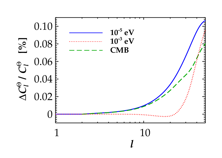
We have found $\tilde{C}_{l}^{\Theta}$ with the lensing code in CAMB and Fig. 8 shows the difference with respect to the unlensed spectra for the $m_{\nu}=10^{-5}$ eV and $10^{-3}$ eV cases, as well as for the CMB. Both neutrino spectra are closely correlated with the CMB case because the main effect is to move power from the higher $l$ modes in the primary spectra which are very similar at these $l$-values. Since the primary spectrum dips to a minimum at a somewhat higher $l$ for $m_{\nu}=10^{-3}$ eV than for $m_{\nu}=10^{-5}$ eV the lensing effect also kicks in later, as can be seen in Fig. 8.

We have not presented lensing results for the higher masses because the relative effect of lensing becomes less important at low $l$, and because numerical noise from the truncation of both primary and lensing spectra at $l=500$ prevents a reliable calculation of the lensed C$\nu$B spectrum much beyond $l\sim 10$ for the most massive cases.

Note that we have found $\tilde{C}_{l}^{\Theta}$ by lensing the average primary spectrum with the average lensing spectrum. For small neutrino masses with $v\simeq c$ this is surely a good approximation. For higher masses it will be more important to lense each $C_{l}^{\Theta}(q)$ with its corresponding $C_{l}^{\Pi}(q)$ and then calculate an energy average, though the order of averaging should not significantly affect the total $\tilde{C}_{l}^{\Theta}$.

References

- [1] E. Komatsu et al. [WMAP Collaboration], Astrophys. J. Suppl. 180, 330 (2009) [arXiv:0803.0547 [astro-ph]].
- [2] J. Hamann, S. Hannestad, G. G. Raffelt and Y. Y. Y. Wong, JCAP 0708, 021 (2007) [arXiv:0705.0440 [astro-ph]].
- [3] F. de Bernardis, A. Melchiorri, L. Verde and R. Jimenez, JCAP 0803, 020 (2008) [arXiv:0707.4170 [astro-ph]].
- [4] K. Ichikawa, T. Sekiguchi and T. Takahashi, Phys. Rev. D 78, 083526 (2008) [arXiv:0803.0889 [astro-ph]].
- [5] J. Hamann, S. Hannestad, A. Melchiorri and Y. Y. Y. Wong, JCAP 0807, 017 (2008) [arXiv:0804.1789 [astro-ph]].
- [6] L. A. Popa and A. Vasile, JCAP 0806, 028 (2008) [arXiv:0804.2971 [astro-ph]].
- [7] S. Bashinsky and U. Seljak, Phys. Rev. D 69, 083002 (2004) [arXiv:astro-ph/0310198].
- [8] R. Trotta and A. Melchiorri, Phys. Rev. Lett. 95, 011305 (2005) [arXiv:astro-ph/0412066].
- [9] N. F. Bell, E. Pierpaoli and K. Sigurdson, Phys. Rev. D 73, 063523 (2006) [arXiv:astro-ph/0511410].
- [10] F. De Bernardis, L. Pagano, P. Serra, A. Melchiorri and A. Cooray, JCAP 0806, 013 (2008) [arXiv:0804.1925 [astro-ph]].
- [11] A. Basboll, O. E. Bjaelde, S. Hannestad and G. G. Raffelt, Phys. Rev. D 79, 043512 (2009) [arXiv:0806.1735 [astro-ph]].
- [12] S. Hannestad, JCAP 0502, 011 (2005) [arXiv:astro-ph/0411475].
- [13] A. Friedland, K. M. Zurek and S. Bashinsky, arXiv:0704.3271 [astro-ph].
- [14] S. Weinberg, Phys. Rev. 128, 1457 (1962).
- [15] A. G. Cocco, G. Mangano and M. Messina, JCAP 0706, 015 (2007) [J. Phys. Conf. Ser. 110, 082014 (2008)] [arXiv:hep-ph/0703075].
- [16] M. Blennow, Phys. Rev. D 77, 113014 (2008) [arXiv:0803.3762 [astro-ph]].
- [17] T. J. Weiler, Phys. Rev. Lett. 49, 234 (1982).
- [18] L. Stodolsky, Phys. Rev. Lett. 34, 110 (1975) [Erratum-ibid. 34, 508 (1975)].
- [19] G. B. Gelmini, Phys. Scripta T121, 131 (2005) [arXiv:hep-ph/0412305].
- [20] A. Ringwald and Y. Y. Y. Wong, JCAP 0412, 005 (2004) [arXiv:hep-ph/0408241].
- [21] Z. Fodor, S. D. Katz and A. Ringwald, JHEP 0206, 046 (2002) [arXiv:hep-ph/0203198].
- [22] G. Duda, G. Gelmini and S. Nussinov, Phys. Rev. D 64, 122001 (2001) [arXiv:hep-ph/0107027].
- [23] P. Langacker, J. P. Leveille and J. Sheiman, Phys. Rev. D 27, 1228 (1983).
- [24] N. Cabibbo and L. Maiani, Phys. Lett. B 114, 115 (1982).
- [25] S. Pastor, G. G. Raffelt and D. V. Semikoz, Phys. Rev. D 65, 053011 (2002) [arXiv:hep-ph/0109035].
- [26] S. Pastor, T. Pinto and G. G. Raffelt, Phys. Rev. Lett. 102, 241302 (2009) [arXiv:0808.3137 [astro-ph]].
- [27] V. Simha and G. Steigman, JCAP 0808, 011 (2008) [arXiv:0806.0179 [hep-ph]].
- [28] Y. Y. Y. Wong, Phys. Rev. D 66, 025015 (2002) [arXiv:hep-ph/0203180].
- [29] K. N. Abazajian, J. F. Beacom and N. F. Bell, Phys. Rev. D 66, 013008 (2002) [arXiv:astro-ph/0203442].
- [30] W. Hu, D. Scott, N. Sugiyama and M. J. . White, Phys. Rev. D 52, 5498 (1995) [arXiv:astro-ph/9505043].
- [31] R. J. Michney and R. R. Caldwell, JCAP 0701, 014 (2007) [arXiv:astro-ph/0608303].
- [32] C. P. Ma and E. Bertschinger, Astrophys. J. 455, 7 (1995) [arXiv:astro-ph/9506072].
- [33] A. Lewis and S. Bridle, Phys. Rev. D 66, 103511 (2002) [arXiv:astro-ph/0205436].
- [34] E. Bertschinger, arXiv:astro-ph/9506070.
- [35] K. M. Gorski, E. Hivon, A. J. Banday, B. D. Wandelt, F. K. Hansen, M. Reinecke and M. Bartelman, Astrophys. J. 622, 759 (2005) [arXiv:astro-ph/0409513].
- [36] S. Dodelson and M. Vesterinen, arXiv:0907.2887 [astro-ph.CO].
- [37] J. Brandbyge and S. Hannestad, [arXiv:0908.1969 [astro-ph]].
- [38] U. Seljak, Astrophys. J. 463, 1 (1996) [arXiv:astro-ph/9505109].
- [39] A. Challinor and A. Lewis, Phys. Rev. D 71 (2005) 103010 [arXiv:astro-ph/0502425].
- [40] A. Lewis and A. Challinor, Phys. Rept. 429 (2006) 1 [arXiv:astro-ph/0601594].
- [41] N. Kaiser, Astrophys. J. 388, 272 (1992) [arXiv:astro-ph/9603033].
- [42] B. Jain and U. Seljak, Astrophys. J. 484, 560 (1997) [arXiv:astro-ph/9611077].