Introduction to Randomness and Statistics
excerpt from the book
Practical Guide to Computer Simulations
World Scientific 2009, ISBN 978-981-283-415-7
see http://www.worldscibooks.com/physics/6988.html
with permission by World Scientific Publishing Co. Pte. Ltd.
Chapter 7 Randomness and Statistics
In this chapter, we are concerned with statistics in a very broad sense. This involves generation of (pseudo) random data, display/plotting of data and the statistical analysis of simulation results.
Frequently, a simulation involves the explicit generation of random numbers, for instance, as auxiliary quantity for stochastic simulations. In this case it is obvious that the simulation results are random as well. Although there are many simulations which are explicitly not random, the resulting behavior of the simulated systems may appear also random, for example the motion of interacting gas atoms in a container. Hence, methods from statistical data analysis are necessary for almost all analysis of simulation results.
This chapter starts (Sec. 7.1) by an introduction to randomness and statistics. In Sec. 7.2 the generation of pseudo random numbers according to some given probability distribution is explained. Basic analysis of data, i.e., the calculation of mean, variance, histograms and corresponding error bars, is covered in Sec. 7.3. Next, in Sec. 7.4, it is shown how data can be represented graphically using suitable plotting tools, gnuplot and xmgrace. Hypothesis testing and how to measure or ensure independence of data is treated in Sec. 7.5. How to fit data to functions is explained in Sec. 7.6. In the concluding section, a special technique is outlined which allows to cope with the limitations of simulations due to finite system sizes.
Note that some examples are again presented using the C programming language. Nevertheless, there exist very powerful freely available programs like R [R], where many analysis (and plotting) tools are available as additional packages.
7.1 Introduction to probability
Here, a short introduction to concepts of probability and randomness is given. The presentation here should be concise concerning the subjects presented in this book. Nevertheless, more details, in particular proofs, examples and exercises, can be found in standard textbooks [Dekking et al (2005), Lefebvre (2006)]. Here often a sloppy mathematical notation is used for brevity, e.g. instead of writing “a function ”, we often write simply “a function ”.
A random experiment is an experiment which is truly random (like radioactive decay or quantum mechanical processes) or at least unpredictable (like tossing a coin or predicting the position of a certain gas atom inside a container which holds a hot dense gas).
Definition The sample space is a set of all possible outcomes of a random experiment.
For the coin example, the sample space is head, tail. Note that a sample space can be in principle infinite, like the possible positions of an atom in a container. With infinite precision of measurement we have , where the container shall be a box with linear extents ( in the other directions, see below).
For a random experiment, one wants to know the probability that certain events occur. Note that for the position of an atom in a box, the probability to find the atom precisely at some -coordinate is zero if one assumes that measurements result in real numbers with infinite precision. For this reason, one considers probabilities of subsets (in other words , being the power set which is the set of all subsets of ). Such a subset is called an event. Therefore is the probability that the outcome of a random experiment is inside , i.e. one of the elements of . More formally:
Definition A probability function is a function with
| (7.1) |
and for each finite or infinite sequence of mutual disjoint events ( for ) we have
| (7.2) |
For a fair coin, both sides would appear with the same probability, hence one has , head, tail, head, tail. For the hot gas inside the container, we assume that no external forces act on the atoms. Then the atoms are distributed uniformly. Thus, when measuring the position of an atom, the probability to find it inside the region is .
The usual set operations applies to events. The intersection of two events is the event which contains elements that are both in and . Hence is the probability that the outcome of an experiment is contained in both events and . The complement of a set is the set of all elements of which are not in . Since , are disjoint and , we get from Eq. (7.2):
| (7.3) |
Furthermore, one can show for two events :
| (7.4) |
Proof . If we apply this for instead of , we get . Eliminating from these two equations gives the desired result.
If a random experiment is repeated several times, the possible outcomes of the repeated experiment are tuples of outcomes of single experiments. Thus, if you throw the coin twice, the possible outcomes are (head,head), (head,tail), (tail,head), and (tail,tail). This means the sample space is a power of the single-experiment sample spaces. In general, it is also possible to combine different random experiments into one. Hence, for the general case, if experiments with sample spaces are considered, the sample space of the combined experiment is . For example, one can describe the measurement of the position of the atom in the hot gas as a combination of the three independent random experiments of measuring the , , and coordinates, respectively.
If we assume that the different experiments are performed independently, then the total probability of an event for a combined random experiment is the product of the single-experiment probabilities: .
For tossing the fair coin twice, the probability of the outcome (head,tail) is head,headheadhead. Similarly, for the experiment where all three coordinates of an atom inside the container are measured, one can write .
Often one wants to calculate probabilities which are restricted to special events among all events, hence relative or conditioned to . For any other event we have , which means . Since is the probability of an outcome in and and because is the probability of an outcome in , the fraction gives the probability of an outcome and relative to , i.e. the probability of event given , leading to the following
Definition The probability of under the condition is
| (7.5) |
As we have seen, we have the natural normalization . Rewriting Eq. (7.5) one obtains . Therefore, the calculation of can be decomposed into two parts, which are sometimes easier to obtain. By symmetry, we can also write . Combining this with Eq. (7.5), one obtains the famous Bayes’ rule
| (7.6) |
This means one of the conditional probabilities and can be expressed via the other, which is sometimes useful if and are known. Note that the denominator in the Bayes’ rule is sometimes written as .
If an event is independent of the condition , its conditional probability should be the same as the unconditional probability, i.e., . Using we get , i.e., the probabilities of independent events have to be multiplied. This was used already above for random experiments, which are conducted as independent subexperiments.
So far, the outcomes of the random experiments can be anything like the sides of coins, sides of a dice, colors of the eyes of randomly chosen people or states of random systems. In mathematics, it is often easier to handle numbers instead of arbitrary objects. For this reason one can represent the outcomes of random experiments by numbers which are assigned via special functions:
Definition For a sample space , a random variable is a function . For example, one could use head=1 and tail. Hence, if one repeats the experiments times independently, one would obtain the number of heads by , where is the outcome of the ’th experiment.
If one is interested only in the values of the random variable, the connection to the original sample space is not important anymore. Consequently, one can consider random variables as devices, which output a random number each time a random experiment is performed. Note that random variables are usually denoted by upper-case letters, while the actual outcomes of random experiments are denoted by lower-case letters.
Using the concept of random variables, one deals only with numbers as outcomes of random experiments. This enables many tools from mathematics to be applied. In particular, one can combine random variables and functions to obtain new random variables. This means, in the simplest case, the following: First, one performs a random experiment, yielding a random outcome . Next, for a given function , is calculated. Then, is the final outcome of the random experiment. This is called a transformation of the random variable . More generally, one can also define a random variable by combining several random variables , …, via a function such that
| (7.7) |
In practice, one would perform random experiments for the random variables , …, , resulting in outcomes , …, . The final number is obtained by calculating . A simple but the most important case is the linear combination of random variables …, which will be used below. For all examples considered here, the random variables , …, have the same properties, which means that the same random experiment is repeated times. Nevertheless, the most general description which allows for different random variables will be used here.
The behavior of a random variable is fully described by the probabilities of obtaining outcomes smaller or equal to a given parameter :
Definition The distribution function of a random variable is a function defined via
| (7.8) |
The index is omitted if no confusion arises. Sometimes the distribution function is also named cumulative distribution function. One also says, the distribution function defines a probability distribution. Stating a random variable or stating the distribution function are fully equivalent methods to describe a random experiment.
For the fair coin, we have, see left of Fig. 7.1
| (7.9) |
For measuring the position of an atom in the uniformly distributed gas we obtain, see right of Fig. 7.1
| (7.10) |

Since the outcomes of any random variable are finite, there are no possible outcomes in the limit . Also, all possible outcomes fulfill for . Consequently, one obtains for all random variables and . Furthermore, from Def. 7.1, one obtains immediately:
| (7.11) |
Therefore, one can calculate the probability to obtain a random number for any arbitrary interval, hence also for unions of intervals.
The distribution function, although it contains all information, is sometimes less convenient to handle, because it gives information about cumulative probabilities. It is more obvious to describe the outcomes of the random experiments directly. For this purpose, we have to distinguish between discrete random variables, where the number of possible outcomes is denumerable or even finite, and continuous random variables, where the possible outcomes are non-denumerable. The random variable describing the coin is discrete, while the position of an atom inside a container is continuous.
7.1.1 Discrete random variables
We first concentrate on discrete random variables. Here, an alternative but equivalent description to the distribution function is to state the probability for each possible outcome directly:
Definition For a discrete random variable , the probability mass function (pmf) is given by
| (7.12) |
Again, the index is omitted if no confusion arises. Since a discrete random variable describes only a denumerable number of outcomes, the probability mass function is zero almost everywhere. In the following, the outcomes where are denoted by . Since probabilities must sum up to one, see Eq. 7.1, one obtains . Sometimes we also write . The distribution funcion is obtained from the pmf via summing up all probabilities of outcomes smaller or equal to :
| (7.13) |
For example, the pmf of the random variable arising from the fair coin Eq. (7.9) is given by and ( elsewhere). The generalization to a possibly unfair coin, where the outcome “1” arises with probability , leads to:
Definition The Bernoulli distribution with parameter () describes a discrete random variable with the following probability mass function
| (7.14) |
Performing a Bernoulli experiment means that one throws a generalized coin and records either “0” or “1” depending on whether one gets head or tail.
There are a couple of important characteristic quantities describing the pmf of a random variable. Next, we describe the most important ones for the discrete case:
Definition
- •
The expectation value is
(7.15) - •
The variance is
(7.16) - •
The standard deviation
(7.17)
The expectation value describes the ‘‘average’’ one would typically obtain if the random experiment is repeated very often. The variance is a measure for the spread of the different outcomes of random variable. As example, the Bernoulli distribution exhibits
| (7.18) | |||||
| (7.19) | |||||
One can calculate expectation values of functions of random variables via . For the calculation here, we only need that the calculation of the expectation value is a linear operation. Hence, for numbers and, in general, two random variables one has
| (7.20) |
In this way, realizing that is a number, one obtains:
| (7.21) | |||||
| (7.22) |
The variance is not linear, which can be seen when looking at a linear combination of two independent random variables (implying ())
| (7.23) | |||||
The expectation values are called the ’th moments of the distribution. This means that the expectation value is the first moment and the variance can be calculated from the first and second moments.
Next, we describe two more important distributions of discrete random variables. First, if one repeats a Bernoulli experiment times, one can measure how often the result “1” was obtained. Formally, this can be written as a sum of random variables which are Bernoulli distributed: with parameter . This is a very simple example of a transformation of a random variable, see page 7.1. In particular, the transformation is linear. The probability to obtain times the result “1” is calculated as follows: The probability to obtain exactly times a “1” is , the other experiments yield “0” which happens with probability . Furthermore, there are different sequences with times “1” and times “0”. Hence, one obtains:
Definition The binomial distribution with parameters and () describes a random variable which has the pmf
| (7.24) |
A common notation is .
Note that the probability mass function is assumed to be zero for argument values that are not stated. A sample plot of the distribution for parameters and is shown in the left of Fig. 7.2. The Binomial distribution has expectation value and variance
| (7.25) | |||||
| (7.26) |
(without proof here). The distribution function cannot be calculated analytically in closed form.


In the limit of a large number of experiments (), constrained such that the expectation value is kept fixed, the pmf of a Binomial distribution is well approximated by the pmf of the Poisson distribution, which is defined as follows: Definition The Poisson distribution with parameter describes a random variable with pmf
| (7.27) |
Indeed, as required, the probabilities sum up to 1, since is the Taylor series of . The Poisson distribution exhibits and . Again, a closed form for the distribution function is not known.
Furthermore, one could repeat a Bernoulli experiment just until the first time a “1” is observed, without limit for the number of trials. If a “1” is observed for the first time after exactly times, then the first times the outcome “0” was observed. This happens with probability . At the ’th experiment, the outcome “1” is observed which has the probability . Therefore one obtains
Definition The geometric distribution with parameter () describes a random variable which has the pmf
| (7.28) |
A sample plot of the pmf (up to ) is shown in the right of Fig. 7.2. The geometric distribution has (without proof here) the expectation value , the variance and the following distribution function:
7.1.2 Continuous random variables
As stated above, random variables are called continuous if they describe random experiments where outcomes from a subset of the real numbers can be obtained. One may describe such random variables also using the distribution function, see Def. 7.1. For continuous random variables, an alternative description is possible, equivalent to the pmf for discrete random variables: The probability density function states the probability to obtain a certain number per unit:
Definition For a continuous random variable with a continuous distribution function , the probability density function (pdf) is given by
| (7.29) |
Consequently, one obtains, using the definition of a derivative and using Eq. (7.11)
| (7.30) | |||||
| (7.31) |
Below some examples for important continuous random variables are presented. First, we extend the definitions Def. 7.1.2 of expectation value and variance to the continuous case:
Definition
- •
The expectation value is
(7.32) - •
The variance is
(7.33)
Expectation value and variance have the same properties as for the discrete case, i.e., Eqs. (7.20), (7.21), and (7.23) hold as well. Also the definition of the n’th moment of a continuous distribution is the same.
Another quantity of interest is the median, which describes the central point of the distribution. It is given by the point such that the cumulative probabilities left and right of this point are both equal to 0.5: Definition The median is defined via
| (7.34) |
The simplest distribution is the uniform distribution, where the probability density function is nonzero and constant in some interval : Definition The uniform distribution, with real-valued parameters , describes a random variable which has the pdf
| (7.35) |
One writes . The distribution function simply rises linearly from zero, starting at , till it reaches 1 at , see for example Eq. 7.10 for the case and . The uniform distribution exhibits the expectation value and variance . Note that via the linear transformation one obtains if . The uniform distribution serves as a basis for the generation of (pseudo) random numbers in a computer, see Sec. 7.2.1. All distributions can be in some way obtained via transformations from one or several uniform distributions, see Secs. 7.2.2–7.2.5.
Probably the most important continuous distribution in the context of simulations is the Gaussian distribution:
Definition The Gaussian distribution, also called normal distribution, with real-valued parameters and , describes a random variable which has the pdf
| (7.36) |
One writes . The Gaussian distribution has expectation value and variance . A sample plot of the distribution for parameters and is shown in the left of Fig. 7.3. The Gaussian distribution for and is called standard normal distribution . One can obtain any Gaussian distribution from by applying the transformation . Note that the distribution function for the Gaussian distribution cannot be calculated analytically. Thus, one uses usually numerical integration or tabulated values of


The central limit theorem describes how the Gaussian distribution arises from a sum of random variables:
Theorem Let , …, be independent random variables, which follow all the same distribution exhibiting expectation value and variance . Then
| (7.37) |
is in the limit of large approximately Gaussian distributed with mean and variance , i.e. .
Equivalently, the suitably normalized sum
| (7.38) |
is approximately standard normal distributed . For a proof, please refer to standard text books on probability. Since sums of random processes arise very often in nature, the Gaussian distribution is ubiquitous. For instance, the movement of a “large” particle swimming in a liquid called Brownian motion is described by a Gaussian distribution.
Another common probability distribution is the exponential distribution. Definition The exponential distribution, with real-valued parameter , describes a random variable which has the pdf
| (7.39) |
A sample plot of the distribution for parameter is shown in the right of Fig. 7.3. The exponential distribution has expectation value and variance . The distribution function can be obtained analytically and is given by
| (7.40) |
The exponential distribution arises under circumstances where processes happen with certain rates, i.e., with a constant probability per time unit. Very often, waiting queues or the decay of radioactive atoms are modeled by such random variables. Then the time duration till the first event (or between two events if the experiment is repeated several times) follows Eq. (7.39).
Next, we discuss a distribution, which has attracted recently [Newman (2003), Newman et al. (2006)] much attention in various disciplines like sociology, physics and computer science. Its probability distribution is a power law:
Definition The power-law distribution, also called Pareto distribution, with real-valued parameters and , describes a random variable which has the pdf
| (7.41) |
A sample power-law distribution is shown in Fig. 7.4. When plotting a power-law distribution with double-logarithmic scale, one sees just a straight line.
A discretized version of the power-law distribution appears for example in empirical social networks. The probability that a person has “close friends” follows a power-law distribution. The same is observed for computer networks for the probability that a computer is connected to other computers. The power-law distribution has a finite expectation value only if , i.e. if it falls off quickly enough. In that case one obtains . Similarly, it exhibits a finite variance only for : . The distribution function can be calculated analytically:
| (7.42) |


In the context of extreme-value statistics, the Fisher-Tippett distribution (also called log-Weibull distribution) plays an important role.
Definition The Fisher-Tippett distribution, with real-valued parameters , describes a random variable which has the pdf
| (7.43) |
In the special case of , the Fisher-Tippett distribution is also called Gumbel distribution. A sample Fisher-Tippett distribution is shown in the right part of Fig. 7.4. The function exhibits a maximum at . This can be shifted to any value by replacing by . The expectation value is , where is the Euler-Mascheroni constant. The distribution exhibits a variance of . Also, the distribution function is known analytically:
| (7.44) |
Mathematically, one can obtain a Gumbel () distributed random variable from standard normal distributed variables by taking the maximum of them and performing the limit , i.e. . This is also true for some other “well-behaved” random variables like exponential distributed ones, if they are normalized such that they have zero mean and variance one. The Fisher-Tippett distribution can be obtained from the Gumbel distribution via a linear transformation.
For the estimation of confidence intervals (see Secs. 7.3.2 and 7.3.3) one needs the chi-squared distribution and the distribution, which are presented next for completeness.
Definition The chi-squared distribution, with degrees of freedom describes a random variable which has the probability density function (using the Gamma function )
| (7.45) |
and for . Distribution function, mean and variance are not stated here. A chi-squared distributed random variable can be obtained from a sum of squared standard normal distributed random variables : The chi-squared distribution is implemented in the GNU scientific library (see Sec. ).
Definition The F distribution, with degrees of freedom describes a random variable which has the pdf
| (7.46) |
and for . Distribution function, mean and variance are not stated here. An F distributed random variable can be obtained from a chi-squared distributed random variable with degrees of freedom and a chi-squared distributed random variable with degrees of freedom via . The F distribution is implemented in the GNU scientific library (see Sec. ).
Finally, note that also discrete random variables can be described using probability density functions if one applies the so-called delta function . For the purpose of computer simulations this is not necessary. Consequently, no further details are presented here.
7.2 Generating (pseudo) random numbers
For many simulations in science, economy or social sciences, random numbers are necessary. Quite often the model itself exhibits random parameters which remain fixed throughout the simulation; one speaks of quenched disorder. A famous example in the field of condensed matter physics are spin glasses, which are random alloys of magetic and non-magnetic materials. In this case, when one performs simulations of small systems, one has to perform an average over different disorder realizations to obtain physical quantities. Each realization of the disorder consists of randomly chosen positions of the magnetic and non-magnetic particles. To generate a disorder realization within the simulations, random numbers are required.
But even when the simulated system is not inherently random, very often random numbers are required by the algorithms, e.g., to realize a finite-temperature ensemble or when using randomized algorithms. In summary, the application of random numbers in computer simulations is ubiquitous.
In this section an introduction to the generation of random numbers is given. First it is explained how they can be generated at all on a computer. Then, different methods are presented for obtaining numbers which obey a target distribution: the inversion method, the rejection method and Box-Müller method. More comprehensive information about these and similar techniques can be found in Refs. [Morgan (1984), Devroye (1986), Press et al. (1995)]. In this section it is assumed that you are familiar with the basic concepts of probability theory and statistics, as presented in Sec. 7.1.
7.2.1 Uniform (pseudo) random numbers
First, it should be pointed out that standard computers are deterministic machines. Thus, it is completely impossible to generate true random numbers directly. One could, for example, include interaction with the user. It is, for example, possible to measure the time interval between successive keystrokes, which is randomly distributed by nature. But the resulting time intervals depend heavily on the current user which means the statistical properties cannot be controlled. On the other hand, there are external devices, which have a true random physical process built in and which can be attached to a computer [Qantis, Westphal] or used via the internet [Hotbits]. Nevertheless, since these numbers are really random, they do not allow to perform stochastic simulations in a controlled and reproducible way. This is important in a scientific context, because spectacular or unexpected results are often tried to be reproduced by other research groups. Also, some program bugs turn up only for certain random numbers. Hence, for debugging purposes it is important to be able to run exactly the same simulation again. Furthermore, for the true random numbers, either the speed of random number generation is limited if the true random numbers are cheap, or otherwise the generators are expensive.
This is the reason why pseudo random numbers are usually taken. They are generated by deterministic rules. As basis serves a number generator function rand() for a uniform distribution. Each time rand() is called, a new (pseudo) random number is returned. (Now the “pseudo” is omitted for convenience) These random numbers should “look like” true random numbers and should have many of the properties of them. One says they should be “good”. What “look like” and “good” means, has to be specified: One would like to have a random number generator such that each possible number has indeed the same probability of occurrence. Additionally, if two generated numbers differ only slightly, the random numbers returned by the respective subsequent calls should differ sustancially, hence consecutive numbers should have a low correlation. There are many ways to specify a correlation, hence there is no unique criterion. Below, the simplest one will be discussed.
The simplest methods to generate pseudo random numbers are linear congruential generators. They generate a sequence of integer numbers between 0 and by a recursive rule:
| (7.47) |
The initial value is called seed.
Here we show a simple C implementation lin_con().
It stores the current number
in the local variable x which is declared as static, such that
it is remembered, even when the function is terminated (see
Sec. ).
There are two arguments. The first
GET SOURCE CODE
DIR: randomness
FILE(S): rng.c
argument set_seed indicates
whether one wants to set a seed. If yes, the new seed should be passed
as second argument, otherwise the value of the second argument is ignored.
The function returns the seed if it is changed, or the new random number.
Note that the constants and are defined inside the function,
while the modulus is implemented via a macro
RNG_MODULUS to make it visible
outside lin_con():
#define RNG_MODULUS  32768                  /* modulus */

int lin_con(int set_seed, int seed)
{
  static int x = 1000;        /* current random number */
  const int a = 12351;                   /* multiplier */
  const int c = 1;                            /* shift */
  if(set_seed)                           /* new seed ? */
    x = seed;
  else                          /* new random number ? */
    x = (a*x+c) % RNG_MODULUS;

  return(x);
}
If you just want to obtain the next random number, you do not care about the
seed. Hence, we use for convenience
rn_lin_con() to call lin_con()
with the first argument being 0:
int rand_lin_con()
{
  return(lin_con(0,0));
}
If we want to set the seed, we also use for convenience a special trivial
function seed_lin_con():
void srand_lin_con(int seed)
{
  lin_con(1, seed);
}
To generate random numbers distributed in the interval one
has to divide the current random number by the modulus . It is desirable to
obtain equally distributed outcomes in the interval, i.e. a uniform
distribution. Random numbers generated from this
distribution can be used as
input to generate random numbers distributed according to other,
basically arbitrary, distributions. Below, you will see
how random numbers obeying other distributions can be generated.
The following simple C function
generates random numbers in using the macro RNG_MODULUS
defined above:
double drand_lin_con()
{
  return( (double) lin_con(0,0) / RNG_MODULUS);
}
One has to choose the parameters in a way that “good” random numbers are obtained, where “good” means “with less correlations”. Note that in the past several results from simulations have been proven to be wrong because of the application of bad random number generators [Ferrenberg et al. (1992), Vattulainen et al. (1994)].
Example To see what “bad generator” means, consider as an example the parameters and the seed value . 10000 random numbers are generated by dividing each of them by . They are distributed in the interval . In Fig. 7.5 the distribution of the random numbers is shown.

The distribution looks rather flat, but by taking a closer look some regularities can be observed. These regularities can be studied by recording -tuples of successive random numbers . A good random number generator, exhibiting no correlations, would fill up the -dimensional space uniformly. Unfortunately, for linear congruential generators, instead the points lie on -dimensional planes. It can be shown that there are at most of the order such planes. A bad generator has much fewer planes. This is the case for the example studied above, see top part of Fig. 7.6


The result for is even worse: only 15 different “random” numbers are generated (with seed 1000), then the iteration reaches a fixed point (not shown in a figure).
If instead is chosen, the two-point correlations look like that shown in the bottom half of Fig. 7.6. Obviously, the behavior is much more irregular, but poor correlations may become visible for higher -tuples.
A generator which has passed several empirical tests is , , . When implementing this generator you have to be careful, because during the calculation numbers are generated which do not fit into 32 bit. A clever implementation is presented in Ref. [Press et al. (1995)]. Finally, it should be stressed that this generator, like all linear congruential generators, has the low-order bits much less random than the high-order bits. For that reason, when you want to generate integer numbers in an interval [1,N], you should use
r = 1+(int) (N*x_n/m);
instead of using the modulo operation as with r=1+(x_n % N).
In standard C, there is a simple built-in random number generator called
rand() (see corresponding documentation), which has
a modulus , which is very poor. On most operating systems,
also drand48()
is available, which is based on
(, ) and needs also special arithmetics. It
is already sufficient for simulations which no not need many random numbers
and do not required highest statistical quality. In recent years,
several high-standard random number generators have been developed.
Several very good ones are included in the
freely availabe GNU scientific library
(see Sec. ). Hence, you do
not have to implement them yourself.
So far, it has been shown how random numbers can be generated which are distributed uniformly in the interval . In general, one is interested in obtaining random numbers which are distributed according to a given probability distribution with some density . In the next sections, several techniques suitable for this task are presented.
7.2.2 Discrete random variables
In case of discrete distributions with finite number of possible outcomes, one can create a table of the possible outcomes together with their probabilities (), assuming that the are sorted in ascending order. To draw a number, one has to draw a random number which is uniformly distributed in and take the entry of the table such that the sum of the probabilities is larger than , but . Note that one can search the array quickly by bisection search: The array is iteratively divided it into two halves and each time continued in that half where the corresponding entry is contained. In this way, generating a random number has a time complexity which grows only logarithmically with the number of possible outcomes. This pays off if the number of possible outcomes is very large.
In exercise (1) you are asked to write a function to sample from the probability distribution of a discrete variable, in particular for a Poisson distribution.
In the following, we concentrate on techniques for generating continuous random variables.
7.2.3 Inversion Method
Given is a random number generator drand() which is assumed to
generate random numbers which are distributed uniformly in . The
aim is to generate random numbers with probability density
. The corresponding distribution function is
| (7.48) |
The target is to find a function , such that after the transformation the outcomes of are distributed according to (7.48). It is assumed that can be inverted and is strongly monotonically increasing. Then one obtains
| (7.49) |
Since the distribution function for a uniformly distributed variable is just (), one obtains . Thus, one just has to choose for the transformation function in order to obtain random numbers, which are distributed according to the probability distribution . Of course, this only works if can be inverted. If this is not possible, you may use the methods presented in the subsequent sections, or you could generate a table of the distribution function, which is in fact a discretized approximation of the distribution function, and use the methods for generating discrete random numbers as shown in Sec. 7.2.2. This can be even refined by using a linearized approximation of the distribution function. Here, we do not go into further details, but present an example where the distribution function can be indeed inverted.
Example Let us consider the exponential distribution with parameter , with distribution function , see page 7.1.2. Therefore, one can obtain exponentially distributed random numbers by generating uniform distributed random numbers and choosing .

GET SOURCE CODE
DIR: random
FILE(S): expo.c
The following simple C function generates a random number which is exponentially distributed. The parameter of the distribution is passed as argument.
double rand_expo(double mu)
{
  double randnum;                  /* random number U(0,1) */
  randnum = drand48();

  return(-mu*log(1-randnum));
}
Note that we use in line 4 the simple drand48()
random number generator, which is included in the C standard library
and works well for applications with moderate statistical requirements.
For more sophisticated generates, see e.g. the GNU scientific library
(see Sec. ).
7.2.4 Rejection Method
As mentioned above, the inversion method works only when the distribution function can be inverted analytically. For distributions not fulfilling this condition, sometimes this problem can be overcome by drawing several random numbers and combining them in a clever way.

The rejection method works for random variables where the pdf fits into a box , i.e., for and . The basic idea of generating a random number distributed according to is to generate random pairs (), which are distributed uniformly in and accept only those numbers where holds, i.e., the pairs which are located below , see Fig. 7.8. Therefore, the probability that is drawn is proportional to , as desired.
GET SOURCE CODE
DIR: randomness
FILE(S): reject.c
The following C function realizes the rejection method for an arbitrary pdf.
It takes as arguments the boundaries of the box y_max, x0
and x1 as well as a pointer pdf
to the function realizing the pdf. For an explanation of function pointers,
see Sec. .
double reject(double y_max, double x0, double x1,
              double (* pdf)(double))
{
  int found;               /* flag if valid number has been found */
  double x,y;               /* random points in [x0,x1]x[0,p_max] */
  found = 0;
  while(!found)                 /* loop until number is generated */
  {
    x = x0 + (x1-x0)*drand48();           /* uniformly on [x0,x1] */
    y = y_max *drand48();               /* uniformly in [0,p_max] */
    if(y <= pdf(x))                                   /* accept ? */
      found = 1;
  }
  return(x);
}
In lines 9–10 the random point, which is uniformly distributed in the box, is generated. Lines 11–12 contain the check whether a point below the pdf curve has been found. The search in the loop (lines 7–13) continues until a random number has been accepted, which is returned in line 14.
Example The rejection method is applied to a pdf, which has density 1 in and rises linearly from 0 to 4 in . Everywhere else it is zero. This pdf is realized by the following C function:
double pdf(double x)
{
  if( (x<0)||
      ((x>=0.5)&&(x<1))||
      (x>1.5) )
      return(0.0);
  else if((x>=0)&&(x<0.5))
      return(1.0);
  else
      return(4.0*(x-1));
}
The resulting empirical histogram pdf is shown in Fig. 7.9.

The rejection method can always be applied if the probability density is boxed, but it has the drawback that more random numbers have to be generated than can be used: If is the area of the box, one has on average to generate auxiliary random numbers to obtain one random number of the desired distribution. If this leads to a very poor efficiency, you can consider to use several boxes for different parts of the pdf.
7.2.5 The Gaussian Distribution
In case neither the distribution function can be inverted nor the probability fits into a box, special methods have to be applied. As an example, a method for generating random numbers distributed according to a Gaussian distribution is considered. Other methods and examples of how different techniques can be combined are collected in [Morgan (1984)].
The probability density function for the Gaussian distribution with mean and variance is shown in Eq. (7.36), see also Fig. 7.10. It is, apart from uniform distributions, the most common distribution occurring in simulations.

Here, the case of a standard Gaussian distribution () is considered. If you want to realize the general case, you have to draw a standard Gaussian distributed number and then use which is distributed as desired.
Since the Gaussian distribution extends over an infinite interval and because the distribution function cannot be inverted, the methods from above are not applicable. The simplest technique to generate random numbers distributed according to a Gaussian distribution makes use of the central limit theorem 7.1.2. It tells us that any sum of independently distributed random variables (with mean and variance ) will converge to a Gaussian distribution with mean and variance . If again is taken to be uniformly distributed in (which has mean and variance ), one can choose and the random variable will be distributed approximately according to a standard Gaussian distribution. The drawbacks of this method are that 12 random numbers are needed to generate one final random number and that numbers larger than 6 or smaller than -6 will never appear.
In contrast to this technique the Box-Müller method is exact. You need two random variables uniformly distributed in to generate two independent Gaussian variables . This can be achieved by generating from and assigning
A proof that and are indeed distributed according to (7.36) can be found e.g. in [Press et al. (1995), Morgan (1984)], where also other methods for generating Gaussian random numbers, some even more efficient, are explained. A method which is based on the simulation of particles in a box is explained in [Fernandez and Criado (1999)]. In Fig. 7.10 a histogram pdf of random numbers drawn with the Box-Müller method is shown. Note that you can find an implementation of the Box-Müller method in the solution of Exercise (3).
7.3 Basic data analysis
The starting point is a sample of measured points …, of some quantity, as obtained from a simulation. Examples are the density of a gas, the transition time between two conformations of a molecule, or the price of a stock. We assume that formally all measurements can be described by random variables representing the same random variable and that all measurements are statistically independent of each other (treating statistical dependencies is treated in Sec. 7.5). Usually, one does not know the underlying probability distribution , having density , which describes .
7.3.1 Estimators
Thus, one wants to obtain information about by looking at the sample …, . In principle, one does this by considering estimators . Since the measured points are obtained from random variables, is a random variable itself. Estimators are often used to estimate parameters of random variables, e.g. moments of distributions. The most fundamental estimators are:
- •
The mean
(7.50) - •
The sample variance
(7.51) The sample standard deviation is .
GET SOURCE CODE
DIR: randomness
FILE(S): mean.c
As example, next a simple C function is shown, which calculates the mean of data points. The function obtains the number of data points and an array containing the data as arguments. It returns the average:
double mean(int n, double *x)
{
  double sum = 0.0;                       /* sum of values */
  int i;                                        /* counter */

  for(i=0; i<n; i++)          /* loop over all data points */
    sum += x[i];
  return(sum/n);
}
You are asked to write a similar function for calculating the variance in exercise (3).
The sample mean can be used to estimate the expectation value of the distribution. This estimate is unbiased, which means that the expectation value of the mean, for any sample sizes , is indeed the expectation value of the random variable. This can be shown quite easily. Note that formally the random variable from which the sample mean is drawn is :
| (7.52) |
Here again the linearity of the expectation value was used. The fact that the estimator is unbiased means that if you repeat the estimation of the expectation value via the mean several times, on average the correct value is obtained. This is independent of the sample size. In general, the estimator for a parameter is called unbiased if .
Contrary to what you might expect due to the symmetry between Eqs. (7.16) and (7.51), the sample variance is not an unbiased estimator for the variance of the distribution, but is biased. The fundamental reason is, as mentioned above, that is itself a random variable which is described by a distribution . As shown in Eq. (7.52), this distribution has mean , independent of the sample size. On the other hand, the distribution has the variance
| (7.53) | |||||
Thus, the distribution of gets narrower with increasing sample size . This has the following consequence for the expectation value of the sample variance which is described by the random variable :
| (7.54) | |||||
This means that, although is biased, is an unbiased estimator for the variance of the underlying distribution of . Nevertheless, also becomes unbiased for .11 1 Sometimes the sample variance is defined as to make it an unbiased estimator of the variance.
For some distributions, for instance a power-law distribution Eq. (7.41) with exponent , the variance does not exist. Numerically, when calculating according Eq. (7.51), one observes that it will not converge to a finite value when increasing the sample size . Instead one will observe occasionally jumps to higher and higher values. One says the estimator is not robust. To get still an impression of the spread of the data points, one can instead calculate the average deviation
| (7.55) |
In general, an estimator is the less robust, the higher the involved moments are. Even the sample mean may not be robust, for instance for a power-law distribution with . In this case one can use the sample median, which is the value such that for half the sample points, i.e. is the ’th sample point if they are sorted in ascending order.22 2 If is even, one can take the average between the ’th and the ’th sample point in ascending order. The sample median is clearly an estimator of the median (see Def. 7.1.2). It is more robust, because it is less influenced by the sample points in the tail. The simplest way to calculate the median is to sort all sample points in ascending order and take the sample point at the ’th position. This process takes a running time . Nevertheless, there is an algorithm [Press et al. (1995), Cormen et al. (2001)] which calculates the median even in linear running time .
7.3.2 Confidence intervals
In the previous section, we have studied estimators for parameters of a random variable using a sample obtained from a series of independent random experiments. This is a so-called point estimator, because just one number is estimated.
Since each estimator is itself a random variable, each estimated value will be usually off the true value . Consequently, one wants to obtain an impression of how far off the estimate might be from the real value . This can be obtained for instance from:
Definition The mean squared error of a point estimator for a parameter is
| (7.56) | |||||
If an estimator is unbiased, i.e., if , the mean squared error is given by the variance of the estimator. Hence, if for independent samples (each consisting of sample points) the estimated values are close to each other, the estimate is quite accurate. Unfortunately, usually only one sample is available (how to circumvent this problem rather ingeniously, see Sec. 7.3.4). Also the mean squared error does not immediately provide a probabilistic interpretation of how far the estimate is away from the true value .
Nevertheless, one can obtain an estimate of the error in a probabilistic sense. Here we want to calculate a so-called confidence interval also sometimes named error bar.
Definition For a parameter describing a random variable, two estimators and which are obtained from a sample …, provide a confidence interval if, for given confidence level we have
| (7.57) |
The value is called conversely significance level. This means, the true but unknown value is contained in the interval , which is itself a random variable as well, with probability . Typical values of the confidence level are 0.68, 0.95 and 0.99 (, , , respectively), providing increasing confidence. The more one wants to be sure that the interval really contains the true parameter, i.e. the smaller the value of , the larger the confidence interval will be.
Next, it is quickly
outlined how one arrives at the confidence interval
for the mean, for details please
consult the specialized literature. First we recall that according
to its definition
the mean is a sum of independent random variables. For computer
simulations, one can assume that usually (see below
for a counterexample) a sufficiently large
number of experiments is performed.33
3
This is different for
many empirical experiments, for example, when testing new treatments
in medical sciences, where often only a very restricted number
of experiments can be performed. In this case, one has to consider
special distributions, like the Student distribution.
Therefore,
according to the central limit theorem
7.1.2
should exhibit (approximately) a pdf
which is Gaussian
with an expectation value and some variance
.
This means, the probability
that the sample means fall outside an
interval
can be easily obtained from the standard normal distribution.
This
situation is shown in the Fig. 7.11.
Note that the interval is symmetric about the mean and that
its width is stated in multiples of the standard deviation
.
The relation between significance level and half
interval width is just .
Hence,
the weight of the standard normal distribution outside
the interval is . This relation
can be obtained from any table
of the standard Gaussian distribution or from the function
gsl_cdf_gaussian_P() of the GNU scientific library
(see Sec. ).
Usually, one considers integer values
which correspond to significance levels , ,
and , respectively.

So far, the confidence interval contains the unknown expectation value and the unknown variance . First, one can rewrite
This now states the probability that the true value, which is estimated by the sample mean , lies within an interval which is symmetric about the estimate . Note that the width is basically given by . This explains why the mean squared error , as presented in the beginning of this section, is a good measure for the statistical error made by the estimator. This will be used in Sec. 7.3.4.
To finish, we estimate the true variance using , hence we get . To summarize we get:
(7.58)
Note that this confidence interval, with and , is symmetric about , which is not necessarily the case for other confidence intervals. Very often in scientific publications, to state the estimate for including the confidence interval, one gives the range where the true mean is located in 68% of all cases () i.e. , this is called the standard Gaussian error bar or one error bar. Thus, the sample variance and the sample size determine the error bar/ confidence interval.
For the variance, the situation is more complicated, because it is not simply a sum of statistically independent sample points …, . Without going into the details, here only the result from the corresponding statistics literature [Dekking et al (2005), Lefebvre (2006)] is cited: The confidence interval where with probability the true variance is located is given by where
(7.59)
Here, is the inverse of the cumulative chi-squared
distribution with degrees of freedom.
It states the value where ,
see page 7.1.2. This chi-squared function
is implemented in the GNU scientific library
(see Sec. ) in the function
gsl_cdf_chisq_Pinv().
Note that as one alternative, you could regard approximately as independent data points and use the above standard error estimate described for the mean of the sample . Also, one can use the bootstrap method as explained below (Sec. 7.3.4), which allows to calculate confidence intervals for arbitrary estimators.
7.3.3 Histograms
Sometimes, you do not only want to estimate moments of an underlying distribution, but you want to get an impression of the full distribution. In this case you can use histograms.
Definition A histogram is given by a set of disjoint intervals
| (7.60) |
which are called bins and a counter for each bin. For a given sample of measured points …, , bin contains the number of sample points which are contained in .
Example For the sample
the bins
are used, resulting in
which is depicted in Fig. 7.12.

In principle, the bins can be chosen arbitrarily. You should take care that the union of all intervals covers all (possible or actual) sample points. Here, it is assumed that the bins are properly chosen. Note also that the width of each bin can be different. Nevertheless, often bins with uniform width are used. Furthermore, for many applications, for instance, when assigning different weights to different sample points44 4 This occurs for some advanced simulation techniques., it is useful to consider the counters as real-valued variables. A simple (fixed-bin width) C implementation of histograms is described in Sec. . The GNU scientific library (see Sec. ) contains data structures and functions which implement histograms allowing for variable bin width.
Formally, for a given random variable , the count in bin can be seen as a result of a random experiment for the binomial random variable with parameters and , where is the probability that a random experiment for results in a value which is contained in bin . This means that confidence intervals for a histogram bin can be obtained in principle from a binomial distribution. Nevertheless, for each sample the true value for a value is unknown and can only be estimated by . Hence, the true binomial distribution is unknown. On the other hand, a binomial random variable is a sum of Bernoulli random variables with parameter . Thus, the estimator is nothing else than a sample mean for a Bernoulli random variable. If the number of sample points is “large” (see below), from the central limit theorem 7.1.2 and as discussed in Sec. 7.3.2, the distribution of the sample mean (being binomial in fact) is approximately Gaussian. Therefore, one can use the standard confidence interval Eq. (7.58), in this case
| (7.61) |
Here, according Eq. (7.19), the Bernoulli random variable exhibits a sample variance . Again, denotes the half width of an interval such that the weight of the standard normal distribution outside the interval equals . Hence, the estimate with standard error bar () is .
The question remains: What is “large” such that you can trust this “Gaussian” confidence interval? Consider that you measure for example no point at all for a certain bin . This can happen easily in the regions where is smaller than but non-zero, i.e. in regions of the histogram which are used to sample the tails of a probability density function. In this case the estimated fraction can easily be resulting also in a zero-width confidence interval, which is certainly wrong. This means, the number of samples needed to have a reliable confidence interval for a bin depends on the number of bin entries. A rule of thumb from the statistics literature is that should hold. If this condition is not fulfilled, the correct confidence interval for has to be obtained from the binomial distribution and it is quite complicated, since it uses the F distribution (see Def. 7.1.2 on page 7.1.2)
| (7.62) | |||||
The value states the value such that the distribution function for the F distribution with number of degrees and reaches the value . This inverse distribution function is implemented in the GNU scientific library (see Sec. ). If you always use these confidence intervals, which are usually not symmetric about , then you cannot go wrong. Nevertheless, for most applications the standard Gaussian error bars are fine.
Finally, in case you want to use a histogram to represent a sample from a continuous random variable, you can easily interpret a histogram as a sample for a probability density function, which can be represented as a set of points . This is called the histogram pdf or the sample pdf. For simplicity, it is assumed that the interval mid points of the intervals are used as -coordinate. For the normalization, we have to divide by the total number of counts, as for and to divide by the bin width. This ensures that the integral of the sample pdf, approximated by a sum, gives just unity. Therefore, we get
| (7.63) |
The confidence interval, whatever type you choose, has to be normalized in the same way. A function which prints a histogram as pdf, with simple Gaussian error bars, is shown in Sec. .
For discrete random variables, the histogram can be used to estimate the pmf.55 5 For discrete random variables, the values are already suitably normalized. In this case the choice of the bins, in particular the bin widths, is easy, since usually all possible outcomes of the random experiments are known. For a histogram pdf, which is used to describe approximately a continuous random variable, the choice of the bin width is important. Basically, you have to adjust the width manually, such that the sample data is respresented “best”. Thus, the bin width should not be too small nor too large. Sometimes a non-uniform bin width is the best choice. In this case no general advice can be given, except that the bin width should be large where few data points have been sampled. This means that each bin should contain roughly the same number of sample points. Several different rules of thumb exist for uniform bin widths. For example [Scott (1979)], which comes from minimizing the mean integrated squared difference between a Gaussian pdf and a sample drawn from this Gaussian distribution. Hence, the larger the variance of the sample, the larger the bin width, while increasing the number of sample points enables the bin width to be reduced.
In any case, you should be aware that the histogram pdf can be only an approximation of the real pdf, due to the finite number of data points and due to the underlying discrete nature resulting from the bins. The latter problem has been addressed in recent years by so-called kernel estimators [Dekking et al (2005)]. Here, each sample point is represented by a so-called kernel function. A kernel function is a peaked function, formally exhibiting the following properties:
- •
It has a maximum at 0.
- •
It falls off to zero over some some distance .
- •
Its integral is normalized to one.
Often used kernel functions are, e.g., a triangle, a cut upside-down parabola or a Gaussian function. Each sample point is represented such that a kernel function is shifted having the maximum at . The estimator for the pdf is the suitably normalized sum (factor ) of all these kernel functions, one for each sample point:
| (7.64) |
The advantages of these kernel estimators are that they result usually in a smooth function and that for a value also sample points more distant from may contribute, with decreasing weight for increasing distance. The most important parameter is the width , because too small a value of will result in many distinguishable peaks, one for each sample point, while too large value a of leads to a loss of important details. This is of similar importance as the choice of the bin width for histograms. The choice of the kernel function (e.g. a triangle, an upside-down parabola or a Gaussian function) seems to be less important.
7.3.4 Resampling using Bootstrap
As pointed out, an estimator for some parameter , given by a function , is in fact a random variable . Consequently, to get an impression of how much an estimate differs from the true value of the parameter, one needs in principle to know the distribution of the estimator, e.g. via the pdf or the distribution function . In the previous chapter, the distribution was known for few estimators, in particular if the sample size is large. For instance, the distribution of the sample mean converges to a Gaussian distribution, irrespectively of the distribution function describing the sample points .
For the case of a general estimator , in particular if is not known, one may not know anything about the distribution of . In this case one can approximate by the sample distribution function:
Definition For a sample , the sample distribution function (also called empirical distribution function) is
| (7.65) |
Note that this distribution function describes in fact a discrete random variable (called here), but is usually (but not always) used to approximate a continuous distribution function.
The bootstrap principle is to use instead of . The name of this principle was made popular by B. Efron [Efron (1979), Efron and Tibshirani (1994)] and comes from the fairy tale of Baron Münchhausen, who dragged himself out of a swamp by pulling on the strap of his boot.66 6 In the European version, he dragged himself out by pulling his hair. Since the distribution function is replaced by the empirical sample distribution function, the approach is also called empirical bootstrap, for a variant called parametric bootstrap see below.
Now, having one could in principle calculate the distribution function for the random variable exactly, which then is an approximation of . Usually, this is to cumbersome and one uses a second approximation: One draws so-called bootstrap samples from the random variable . This is called resampling. This can be done quite simply by times selecting (with replacement) one of the data points of the original sample , each one with the same probability . This means that some sample points from may appear several times in , some may not appear at all.77 7 The probability for a sample point not to be selected is for . Now, one can calculate the estimator value for each bootstrap sample. This is repeated times for different bootstrap samples resulting in values () of the estimator. The sample distribution function of this sample is the final result, which is an approximation of the desired distribution function . Note that the second approximation, replacing by can be made arbitrarily accurate by making as large as desired, which is computationally cheap.
You may ask: Does this work at all, i.e., is a good approximation of ? For the general case, there is no answer. But for some cases there are mathematical proofs. For example for the mean the distribution function in fact converges to . Here, only the subtlety arises that one has to consider in fact the normalized distributions of () and (). Thus, the random variables are just shifted by constant values. For other cases, like for estimating the median or the variance, one has to normalize in a different way, i.e., by subtracting the (empirical) median or by dividing by the (empirical) variance. Nevertheless, for the characteristics of we are interested in, in particular in the variance, see below, normalizations like shifting and stretching are not relevant, hence they are ignored in the following. Note that indeed some estimators exist, like the maximum of a distribution, for which one can prove conversely that does not converge to , even after some normalization. On the other hand, for the purpose of getting a not too bad estimate of the error bar, for example, bootstrapping is a very convenient and suitable approach which has received high acceptance during recent years.
Now one can use to calculate any desired quantity. Most important is the case of a confidence interval such that the total probability outside the interval is , for given significance level , i.e. . In particular, one can distribute the weight equally below and above the interval, which allows to determine
| (7.66) |
Similar to the confidence intervals presented in Sec. 7.3.2, also represents a confidence interval for the unknown parameter which is to be estimated from the estimator (if it is unbiased). Note that can be non-symmetric about the actual estimate . This will happen if the distribution is skewed.
For simplicity, as we have seen in Sec. 7.3.2, one can use the variance to describe the statistical uncertainty of the estimator. As mentioned on page 7.3.2, this corresponds basically to a uncertainty.
GET SOURCE CODE
DIR: randomness
FILE(S): bootstrap.c
bootstrap_test.c
The following C function
calculates , as approximation of
the unknown . One has to pass as arguments
the number of sample points,
an array containing the sample points, the number
of bootstrap iterations, and a pointer to the function
f which represents the estimator. f has to take two arguments:
the number of sample points and an array containing a sample.
For an explanation of function pointers, see Sec. .
The function bootstrap_variance() returns .
double bootstrap_variance(int n, double *x, int n_resample,
                         double (*f)(int, double *))
{
  double *xb;                                  /* bootstrap sample */
  double *h;                            /* results from resampling */
  int sample, i;                                  /* loop counters */
  int k;                                        /* sample point id */
  double var;                             /* result to be returned */
  h = (double *) malloc(n_resample * sizeof(double));
  xb = (double *) malloc(n * sizeof(double));
  for(sample=0; sample<n_resample; sample++)
  {
    for(i=0; i<n; i++)                                 /* resample */
    {
      k = (int) floor(drand48()*n);         /* select random point */
      xb[i] = x[k];
    }
    h[sample] = f(n, xb);                   /* calculate estimator */
  }
  var = variance(n_resample, h);      /* obtain bootstrap variance */
  free(h);
  free(xb);
  return(var);
}
The bootstrap samples are stored in the array xb, while
the sampled estimator values are stored in the array h.
These arrays are allocated in lines 10–11.
In the main loop (lines 12–20) the bootstrap samples
are calculated, each time the estimator is obtained and the
result is stored in h. Finally, the variance of the sample
is calculated (line 22). Here, the function
variance() is used, which works similarly to the
function mean(), see exercise (3).
Your are asked to implement a bootstrap function for general
confidence interval in exercise (4).
The most obvious way is to call bootstrap_variance() with the
estimator mean as forth argument.
For a distribution which is “well behaved”
(i.e., where a sum of few random variables resembles the
Gaussian distribution),
you will get a variance that is,
at least if n_resample is reasonably large, very close
to the standard Gaussian () error bar.
For calculating properties of the sample mean, the bootstrap approach works fine, but in this case one could also be satisfied with the standard Gaussian confidence interval. The bootstrap approach is more interesting for non-standard estimators. One prominent example from the field of statistical physics is the so-called Binder cumulant [Binder (1981)], which is given by:
| (7.67) |
GET SOURCE CODE
DIR: randomness
FILE(S): binder_L8.dat
binder_L10.dat
binder_L16.dat
binder_L30.dat
where is again the sample mean, for example . The Binder cumulant is often used to determine phase transitions via simulations, where only systems consisting of a finite number of particles can be studied. For example, consider a ferromagnetic system held at some temperature . At low temperature, below the Curie temperature , the system will exhibit a macroscopic magnetization . On the other hand, for temperatures above , will on average converge to zero when increasing the system size. This transition is fuzzy, if the system sizes are small. Nevertheless, when evaluating the Binder cumulant for different sets of sample points which are obtained at several temperatures and for different system sizes , the curves for different will all cross [Landau and Binder (2000)] (almost) at , which allows for a very precise determination of . A sample result for a two-dimensional (i.e. layered) model ferromagnet exhibiting particles is shown in Fig. 7.13. The Binder cumulant has been useful for the simulation of many other systems like disordered materials, gases, optimization problems, liquids, and graphs describing social systems.

A confidence interval for the Binder cumulant
is very difficult (or even impossible) to obtain using standard
error analysis. Using bootstrapping, it is straightforward. You can
use simply the function bootstrap_variance() shown above
while providing as argument a function which evaluates the Binder
cumulant for a given set of data points.
So far, it was assumed that the empirical distribution function was used to determine an approximation of . Alternatively, one can use some additional knwoledge which might be available. Or one can make additional assumptions, via using a distribution function which is parametrized by a vector of parameters . For an exponential distribution, the vector would just consist of one parameter, the expectation value, while for a Gaussian distribution, would consist of the expectation value and the variance. In principle, arbitrary complex distributions with many parameters are possible. To make a “good” approximation of , one has to adjust the parameters such that the distribution function represents the sample “best”, resulting in a vector of parameters. Methods and tools to perform this fitting of parameters are presented in Sec. 7.6.2. Using one can proceed as above: Either one calculates exactly based on , which is most of the time too cumbersome. Instead, usually one performs simulations where one takes repeatedly samples from simulating and calculates each time the estimator . This results, as in the case of the empirical bootstrap discussed above, in a sample distribution function which is further analyzed. This approach, where is used instead of , is called parametric bootstrap.
Note that the bootstrap approach does not require that the sample points are statistically independent of each other. For instance, the sample could be generated using a Markov chain Monte Carlo simulation [Newman and Barkema (1999), Landau and Binder (2000), Robert and Casella (2004), Liu (2008)], where each data point is calculated using some random process, but also depends on the previous data point . More details on how to quantify correlations are given in Sec. 7.5. Nevertheless, if the sample follows the distribution , everything is fine when using bootstrapping and for example a confidence interval will not depend on the fraction of “independent” data points. One can see this easily by assuming that you replace each data point in the original sample by ten copies, hence making the sample ten times larger without adding any information. This will not affect any of the following bootstrap calculations, since the size of the sample does not enter explicitly. The fact that bootstrapping is not susceptible to correlations between data points is in contrast to the classical calculation of confidence intervals explained in Sec. 7.3.2, where independence of data is assumed and the number of independent data points enters formulas like Eq. (7.58). Hence, when calculating the error bar according to Eq. (7.58) using the ten-copy sample, it will be incorrectly smaller by a factor , since no additional information is available compared to the original sample.
It should be mentioned that bootstrapping is only one of several resampling techniques. Another well known approach is the jackknife approach, where one does not sample randomly using or a fitted . Instead the sample is divided into blocks of equal size (assuming that is a multiple of ). Note that choosing is possible and not uncommon. Next, a number of so-called jackknife samples are formed from the original sample by omitting exactly the sample points from the ’th block and including all other points of the original sample. Therefore, each of these jackknife samples consists of sample points. For each jackknife sample, again the estimator is calculated, resulting in a sample of size . Note that the sample distribution function of this sample is not an approximation of the estimator distribution function ! Nevertheless, it is useful. For instance, the variance can be estimated from , where is the sample variance of . No proof of this is presented here. It is just noted that when increasing the number of blocks, i.e., making the different jackknife samples more alike, because fewer points are excluded, the sample of estimators values will fluctuate less. Consequently, this dependence on the number of blocks is exactly compensated via the factor . Note that for the jackknife method, in contrast to the boostrap approach, the statistical independence of the original sample is required. If there are correlations between the data points, the jackknife approach can be combined with the so-called blocking method [Flyvbjerg (1998)]. More details on the jackknife approach can be found in [Efron and Tibshirani (1994)].
Finally, you should be aware that there are cases where resampling approaches clearly fail. The most obvious example is the calculation of confidence intervals for histograms, see Sec. 7.3.3. A bin which exhibits no sample points, for example, where the probability is very small, will never get a sample point during resampling either. Hence, the error bar will be of zero width. This is in contrast to the confidence interval shown in Eq. 7.62, where also bins with zero entries exhibit a finite-size confidence interval. Consequently, you have to think carefully before deciding which approach you will use to determine the reliability of your results.
7.4 Data plotting
So far, you have learned many methods for analyzing data. Since you do not just want to look at tables filled with numbers, you should visualize the data in viewgraphs. Those viewgraphs which contain the essential results of your work can be used in presentations or publications. To analyze and plot data, several commercial and non-commercial programs are available. Here, two free programs are discussed, gnuplot, and xmgrace. Gnuplot is small, fast, allows two- and three-dimensional curves to be generated and transformed, as well as arbitrary functions to be fitted to the data (see Sec. 7.6.2). On the other hand xmgrace is more flexible and produces better output. It is recommended to use gnuplot for viewing and fitting data online, while xmgrace is to be preferred for producing figures to be shown in presentations or publications.
7.4.1 gnuplot
The program gnuplot is invoked by entering gnuplot in a shell, or from a menu of the graphical user interface of your operating system. For a complete manual see [Texinfo].
As always, our examples refer to a UNIX window system like X11, but the program is available for almost all operating systems. After startup, in the window of your shell or the window which pops up for gnuplot the prompt (e.g. gnuplot) appears and the user can enter commands in textual form, results are shown in additional windows or are written into files. For a general introduction you can type just help.
Before giving an example, it should be
pointed out that gnuplot scripts
can be generated by simply writing the commands
into a file, e.g. command.gp, and calling
gnuplot command.gp.
GET SOURCE CODE
DIR: randomness
FILE(S): sg_e0_L.dat
The typical case is that you have available a data file of data or with data (where is the error bar of the data points). Your file might look like this, where the “energy” of a system88 8 It is the ground-state energy of a three-dimensional spin glass , a protypical system in statistical physics. These spin glasses model the magnetic behavior of alloys like iron-gold. is stored as a function of the “system size” . The filename is sg_e0_L.dat. The first column contains the values, the second the energy values and the third the standard error of the energy. Please note that lines starting with “#” are comment lines which are ignored on reading:
# ground state energy of +-J spin glasses
# L    e_0   error
  3 -1.6710 0.0037
  4 -1.7341 0.0019
  5 -1.7603 0.0008
  6 -1.7726 0.0009
  8 -1.7809 0.0008
 10 -1.7823 0.0015
 12 -1.7852 0.0004
 14 -1.7866 0.0007
To plot the data enter
gnuplot> plot "sg_e0_L.dat" with yerrorbars
which can be abbreviated as p "sg_e0_L.dat" w e. Please do not forget the quotation marks around the file name. Next, a window pops up, showing the result, see Fig. 7.14.
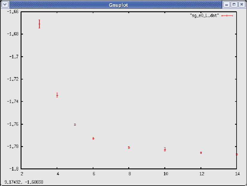
For the plot command many options and styles are available, e.g. with lines produces lines instead of symbols. It is not explained here
how to set line styles or symbol sizes and colors, because this
is usually not necessary for a quick look at the data. For “nice” plots
used for presentations, we recommend xmgrace, see next section.
Anyway, help plot will tell you all you have to know
about the plot command.
Among the important options of the plot command is that one can specify ranges. This can be done by specifying the range directly after the command, e.g.
gnuplot> plot [7:20] "sg_e0_L.dat" with yerrorbars
will only show the data for . Also an additional range can be specified like in
plot [7:20][-1.79:-1.77] "sg_e0_L.dat" with yerrorbars
If you just want to set the range, you have to specify [ ]
for the -range. You can also fix the ranges via the set xrange
and the set yrange commands, such that you do not have to give them each
time with the plot command, see help set xrange or
help unset xrange for unsetting a range.
Gnuplot knows a lot of built-in functions like ,
, powers, roots, Bessel functions, error function,99
9
The
error function is erf.
and many more. For a complete list type help functions.
These function can be also plotted. Furthermore,
using these functions and standard arithmetic expressions, you
can also define your own functions, e.g. you can define a function
ft(x) for the Fischer-Tippett pdf (see Eq. (7.43))
for parameter (called lambda here) and show the function
via
gnuplot> ft(x)=lambda*exp(-lambda*x)*exp(-exp(-lambda*x))
gnuplot> lambda=1.0
gnuplot> plot ft(x)
You can also include arithmetic expressions in the plot command. To plot a shifted and scaled Fischer-Tippett pdf you can type:
gnuplot> plot [0:20] 0.5*ft(0.5*(x-5))
The Fischer-Tippett pdf has a tail which drops off exponentially. This can be better seen by a logarithmic scaling of the axis.
gnuplot> set logscale y
gnuplot> plot [0:20] 0.5*ft(0.5*(x-5))
will produce the plot shown in Fig. 7.15.
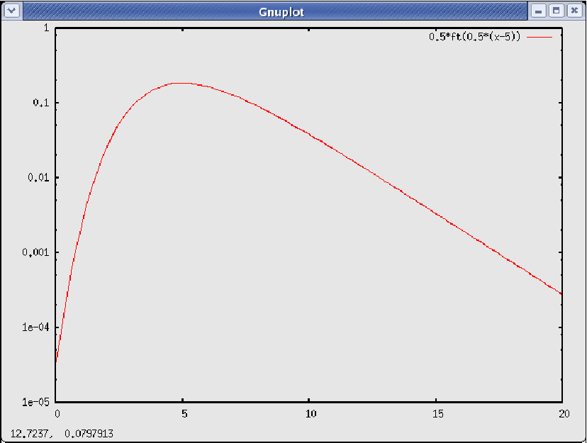
Furthermore, it is also possible to plot several functions in
one plot, via separating them via commas, e.g. to compare a
Fischer-Tippett pdf to the standard Gaussian pdf, here the
predefined constant pi is used:
gnuplot> plot ft(x), exp(-x*x/2)/sqrt(2*pi)
It is possible to read files with multi columns via the using data modifier, e.g.
gnuplot> plot "test.dat" using 1:4:5 w e
displays the fourth column as a function of the first, with error bars
given by the 5th column. The elements behind the using are called
entries.
Within the using data modifier
you can also perform transformations and calculations.
Each entry, where some calculations
should be performed have to be embraced in ( ) brackets.
Inside the brackets you can refer to the different columns of the input
file via $1 for the first column, $2 for the second, etc.
You can generate arbitrary expressions inside the brackets, i.e. use data from different columns (also combine several columns in one entry),
operators, variables,
predefined and self-defined functions and so on. For example, in
Sec. 7.6.2, you will see that the data from
the sg_e0_L.dat file follows
approximately a power law behavior with
, and . To visualize
this, we want to show as a function of .
This is accomplished via:
gnuplot> einf=-1.788
gnuplot> b=-2.8
gnuplot> plot "sg_e0_L.dat" u ($1**b):($2-einf)
Now the gnuplot window will show the data as a straight line (not shown, but see Fig. 7.23).
So far, all output has appeared on the screen. It is possible to redirect the output, for example, to an encapsulated postscript file (by setting set terminal postscript and redirecting the output set output "test.eps"). When you now enter a plot command, the corresponding postscript file will be generated.
Note that not only several functions but also several data
files or a mixture of both can be combined into
one figure.
To remember what a plot exported to files means,
you can set axis labels of the figure by
typing e.g. set xlabel "L", which becomes active when the next
plot command is executed. Also you can use set title
or place arbitrary labels via set label. Use the help
command to find out more.
Also three-dimensional plotting (in fact a projection into two dimensions) is possible using the splot command (enter help splot to obtain more information). Here, as example, we plot a two-dimensional Gaussian distribution:
gnuplot> x0=3.0
gnuplot> y0=-1.0
gnuplot> sx=1.0
gnuplot> sy=5.0
gnuplot> gauss2d(x,y)=exp(-(x-x0)**2/(2*sx)-(y-y0)**2/(2*sy))\
> /sqrt(4*pi**2*sx**2*sy**2)
gnuplot> set xlabel "x"
gnuplot> set ylabel "y"
gnuplot> splot [x0-2:x0+2][y0-4:y0+4]  gauss2d(x,y) with points
gnuplot>
Note that the long line containing the definition of the (two-argument)
function gauss2d() is split up into two lines using a backslash
at the end of the first line. Furthermore, some of the variables are
used inside the interval specifications at the beginning of the
splot command. Clearly, you also can plot
data files with three-dimensional data.
The resulting plot appearing in the output window
is shown in Fig. 7.16.
You can drag the mouse inside the window showing the plot,
which will alter the view.
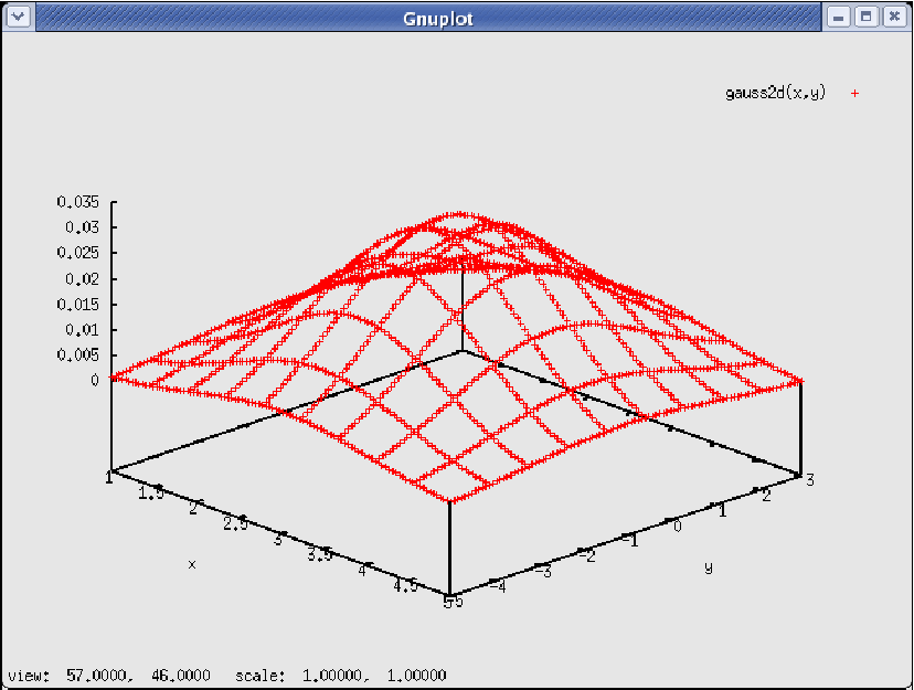
Finally, to stop the execution of gnuplot, enter the
command exit. These examples should give you already a good
impression of what can be done with gnuplot. More can be found
in the documentation or the online help.
How to fit functions to data using gnuplot
is explained in Sec. 7.6.2.
It is also possible to make,
with some effort, publication-suitable plots, but it is simpler
to achieve this with xmgrace, which is presented in the following
section.
7.4.2 xmgrace
The xmgrace (X Motiv GRaphing, Advanced Computation and
Exploration of data) program is much more powerful than
gnuplot and produces nicer output, commands are issued by clicking on
menus and buttons and it offers WYSIWYG.
The xmgrace program offers almost every feature you can imagine for
two-dimensional data plots, including multiple plots (insets),
fits, fast Fourier transform, interpolation. The look of the plots may be
altered in any kind of way you can imagine like choosing fonts,
sizes, colors, symbols, styles for lines, bar charts etc. Also, you can create
manifold types of labels / legends and it is possible to add elements
like texts, labels, lines or other geometrical objects in the plot.
The plots can be exported to various format, in particular encapsulated
postscript (.eps)
Advanced users also can program it or use it for real-time visualization
of simulations.
On the other hand, its handling is a little bit
slower compared to gnuplot
and the program has the tendency to fill your screen with windows.
For full
information, please consult the online help, the manual or the
program’s web page [xmgrace].

Here, just the main steps to produce a simple but nice plot are shown
and some further directions are mentioned.
You will be given here the most important steps
to create a similar plot to the first example, shown for
the gnuplot program, but ready for publication.
First you have to
start the program
by typing xmgrace into a shell (or to start it from some
window/operating system menu). Then you choose the
Data menu1010
10
The underlined character appears
also in the menu name and refers to the key one has to hit together
with Alt button, if one wants
to open the menu via key strokes., next
the Import sub menu
and finally the ASCII.. sub sub menu.
Then a “Grace:Read Set”
window will pop up (see Fig. 7.17)
and you can choose the data file to be loaded
(here sg_e0_L.dat) [A], the type of the input file
(Single Set) [B],
the format of the data (XYDY) [C]. This means you have
three columns, and the third one is an error bar for the second.
Then you can hit on the
OK button [E]. The data will be loaded and shown in the
main window (see Fig. 7.18).
The axis ranges have been adjusted to the data, because
the “Autoscale on read” is set by default to “XY” [D].
You can quickly change the part of the data shown by the buttons
(magnifier, AS, Z, z, , ,
, ) on the left of the main window just below
the Draw button.

Note that another important input file type is “Block data” where the files consist of many columns of which you only want to show some. When you hit th OK button [E], another window (Grace:Edit block data) will pop up, where you have to select the columns which you actually want to display. For the data format (also when loading block data), some other important choices are XY (no error bars) and XYDYDY (full confidence interval, maybe non-symmetric). Finally, you can close the file selection window, by hitting on the Cancel button [F]. The OK and Cancel buttons are common to all xmgrace windows and will not be mentioned explicitly in the following.
In the form the loaded data is shown by default, it is not suitable
for publication purposes, because the symbols, lines and fonts are usually
too small/ too thin. To adjust many details of your graph, you should
go to the Plot menu. First, you choose the
Plot appearance…
sub menu. A corresponding window will pop up.
Here, you should just unselect the “Fill” toggle box (upper right
corner), because otherwise the bounding box included in the .eps
file will not match the plot and your figure will overwrite other parts
of e.g. your manuscript. The fact that your plot has no background now
becomes visible through the appearance of some small dots in the main
xmgrace window, but this does not disrupt the output when exporting
to .eps.

Next, you choose the Set appearance… sub menu from the Plot menu. The corresponding window will pop up, see Fig. 7.19. You can pop this window also by double-clicking inside the graph. This window allows to change the actual display style of the data. You have to select the data set or sets [A] to which the changes will be be applied to when hitting the Apply button at the lower left of the window. Note that the list of sets in this box will contain several sets if you have imported more than one data set. Each of them can have (and usually should) its own style. The box where the list of sets appears is also used to administrate the sets. If you hit the right mouse button, while the mouse pointer is inside this box, a menu will pop up, where you can for instance copy or delete sets, hide or unhide them, or rearrange them.
The options in this window are arranged within different tabs, the most important is the “Main” tab [B]. Here you can choose whether you want to show symbols for your data points and which type [C], also the symbol sizes and colors. If you want to show lines as well (Line properties area at the right), you can choose the style like “straight” and others, but also “none” is no lines should be displayed. The style can be full, dotted, dashed, and different dotted-dashed styles. For presentations and publications it is important that lines are well visible, in this example a line width of 2 is chosen [D] and a black color [E]. For presentations you can distinguish different data sets also by different colors, but for publications in scientific journals you should keep in mind that the figures are usually printed in black and white, hence light colors are not visible.1111 11 Acting as referee reading scientific papers submitted to journals, I experienced many times that I could not recognize or distinguish some data because they were obviously printed in a light color, or with a thin line width, or with tiny symbols ….
Each data set can have a legend (see below how to activate it). Here, the
legend string can be stated. You can enter it directly, with the
help of some formatting commands which are characters preceded by
a backslash \ . The most important ones are
- •
\\prints a backslash. - •
\0selects the Roman font, which is also the default font. A font is active until a new one is chosen. - •
\1selects the italic font, used in equations. - •
\xselects a symbol font, which contains e.g. Greek characters. For example\xabchqLwill generate , just to mention some important symbols. - •
\sgenerates a subscript, while\Nswitches back to normal. For example\xb\s2\N\1(x)generates . - •
\Sgenerates a superscript, for instance\1A\S3x\N-5generates . - •
The font size can be changed with
\+and\-. - •
With
\oand\Oone can start and stop overlining, respectively, for instance\1A\oBC\ODgenerates . Underlining can be controlled via\uand\U.
By default, error bars are shown (toggle box lower right corner). At least you should increase the line width for the symbols (Symbols tab) and increase the base and rise line widths for error bars (Error bars tab).
You should know that, when you are creating another plot, you do not have to redo all these and other adjustments of styles. Once you have found your standard, you can save it using the Save Parameters… sub menu from the Plot menu. You can conversely load a parameter set via the Load Parameters… sub menu of the same menu.

Next, you can adjust the properties of the axes, by choosing the Set appearance… sub menu from the Plot menu or by double-clicking on an axis. The corresponding window will pop up, see Fig. 7.20. You have to select the axis where the current changes apply to [A]. For the axis you should set the range in the fields Start [B] and Stop [C], here to the values 1 and 15. Below these two fields you find the important Scale field, where you can choose linear scaling (default), logarithmic or reciprocal, to mention the important ones.
The most important adjustments you can perform within the
Main tab [D]. Here you enter the label shown below the axis
in the Label string field [E]. The format of the
string is the same as for the data set legends. Here you enter
just \1L, which will show as . The major spacing of the major
(with labels) and minor ticks can be chosen in the corresponding fields
[F,G]. Below there is a Format field, where you can
choose how the tick labels are printed. Among the many formats,
the most common are General (),
Exponential (1.0e+00, 5.0e+00, 1.0e+01,…),
and Power, which is useful for logarithmic scaled axes
(). For the tick labels, you can also choose
a Precision.
This and other fields of this tab you can leave at their
standard values here.
Nevertheless, you should also adjust the Char size of the axis labels
(tab Axis label & bar) and of the tick labels (tab
Tick labels). For publications, character sizes above 150%
are usually well readable.
Note that in the Axis label & bar tab, there is a field
Axis transform where you can enter formulas to transform the
axis more or less arbitrarily, see the manual for details.
All tabs have many other fields, which
are useful as well, but here we stay with the standard
choices. Note that sometimes the Special tab is useful, where you can
enter all major and minor ticks individually.
To finish the design of the axes, you can perform similar changes
to the axis, with Start field , Stop field ,
Label string field \1E\s0\N(L) and the same character sizes
as for the axis for axis labels and tick labels in the corresponding tabs.
Note that the axis label will be printed vertically. If you do not like
this, you can choose the Perpendicular to axis orientation
in the Layout field of the Axis label & bar tab.
Now you have already a nice graph. To show you some more of the capabilities of xmgrace, we refine it a bit. Next, you generate an inset, i.e. a small subgraph inside the main graph. This is quite common in scientific publications. For this purpose, you select the underlineEdit menu and there the Arrange graph… sub menu. The corresponding window appears. We want to have just one inset, i.e. in total 2 graphs. For this purpose, you select in the Matrix region of the window the Cols: field to 1 and the Rows: field to 2. Then you hit on the Accept button which applies the changes and closes the window. You now have two graphs, one containing the already loaded data, the other one being empty. These two graphs are currently shown next to each other, one at the top and one at the bottom.

To make the second graph an inset of the
first, you choose the Graph appearance… sub menu from the
Plot menu. At the top a list of the available graphs
is shown [A]. Here you select the first graph G0.
You need only the Main tab [B], other tabs are for changing
styles of titles, frames and legends. We recommend to choose
Width 2 in the Frame tab.
In the Main tab, you can choose the Type of graph [C],
e.g. XY graph, which we use here (default),
Polar graph or Pie chart. You only have to change the
Viewport coordinates [D] here. These coordinates
are relative coordinates, i.e. the standard full viewport including
axes, labels and titles is .
For the main graph G0,
you choose Xmin and Ymin 0.15 and Xmax and Ymax 0.85.
Note that below there is a toggle box Display legend [E],
where you can control whether a legend is displayed. If you want to have
a legend, you can control its position in the Leg. box tab.
Now the different graphs overlap. This does not bother you, because
next you select graph G1 in the list at the top of the window.
We want to have the inset in the free area of the plot, in the upper right
region. Thus, you enter the viewport coordinates Xmin 0.38,
Ymin 0.5, Xmax 0.8 and Ymax 0.8.

Now the second graph is well placed, but empty.
We want to show a scaled version
of the data in the inset. Hence, you import the data again in the same way
as explained above, while
choosing Read to graph G1 in the Grace: Read sets window.
In Sec. 7.6.2, you will see that the data follows
approximately a power law behavior with
, and . To visualize
this, we want to show as a function of .
Hence, we want to transform the data. You choose from
the Data menu the Transformations sub menu
and there the Evaluate expression sub sub menu. Note that here
you can
also find many other transformations, e.g. Fourier transform, interpolation
and curve fitting. Please consult the manual for details.
In this case, the evaluateExpression window pops up, see
Fig. 7.22 (if you did not close
the windows you have used before, your screen will be already pretty
populated). A transformation always takes the data points
from one source set, applies a formula to all data points (or to a subset
o points) and stores the result in a destination set. These
sets can be selected at the top of the window in the Source [A]
and Destination [B] fields for graph and set separately.
Note that the
data in the destination set is overwritten. If you want to write the
transformed data to a new set, you can first copy an existing set
(click on the right mouse button in the Destination Set window
and choose Duplicate). In our case, we want to replace the data,
hence you select for source and destination the data set from graph
G1. The transformation is entered below [C], here you
first enter y=y+1.788 to shift the data. The you hit the
Apply button at the bottom. Next you change the transformation to
x=x^(-2.8) and hit the
Apply button again. When you now select the second graph by clicking
into it, and hit the AS (auto scale) button on the left
of the main window, you will see that the data points follow a
nice straight line in the inset,
which confirms the behavior of the data.

Again you should select symbols, line stiles, and axis labels
for the inset. Usually smaller font sizes are used here. Note that all
operations always apply to the current graph, which can
be selected for example
by clicking near the corners of the boundary boxes of the graph (which does
not always work, depending on which other windows are open) or by double
clicking on the corresponding graph in the graph list in the
Grace: Graph Appearance window. The final main window
is shown in Fig. 7.23. Note that the left axis label
is not fully visible. This is no problem when exporting the file
as encapsulated postscript; everything will be shown.
But if you do not like it,
you can adjust the Xmin value of graph G0.
Finally, if you choose the menu Window and the sub menu Drawing objects a window will pop up which enable many graphical elements like texts, lines, boxes and ellipses (again with a variety of choices for colors, styles, sizes etc.) tobe added/changed and deleted in your plot. We do not go into details here.
Now you should save your plot using the File menu and
the Save as… sub menu, e.g. with file
name sg_e0_L.agr, where .agr is the typical postfix
of xmgrace source files. When
GET SOURCE CODE
DIR:
randomness
FILE(S): sg_e0_L.dat
you want to create another plot
with similar layout later, it is convenient to start from this saved file
by copying it to a new file
and subsequently using again xmgrace to modify the new file.
To export your file as encapsulated postscript, suitable for including
it into presentations or publications (see Sec. ),
you have to choose the File menu and
the Print setup… sub menu. In the window, which pops
up, you can select the Device EPS. The file name
will automatically switch to sg_e0_L.eps (this seems not to work
always,
in particular if you edit several files, one after the other, please
check the file names always). Having
hit on the Accept button, you can select the File menu and
the Print sub menu, which will generate
the desired output file.1212
12
Using the tool epstopdf
you can convert the postcript file also to a pdf file.
With other tools like convert or gimp you can
convert to many other styles.
Now you have a solid base for viewing and plotting, hence we can continue with advanced analysis techniques. You can experiment with plotting using xmgrace in exercise (5).
7.5 Hypothesis testing and (in-)dependence of data
In the previous section, you have learned how to visualized data, mainly data resulting from the basic analysis methods presented in Sec. 7.3. In this section, we proceed with more elaborate analysis methods. One important way to analyze data of simulations is to test hypotheses concerning the results. The hypothesis to be tested is usually called null hypothesis H0. Examples for null hypotheses are:
- (A)
In a traffic system, opening a new track will decrease the mean value of the travel time for a connection AB below a target threshold .
- (B)
Within an acquaintance network, a change of the rules describing how people meet will change the distribution of the number of people each person knows.
- (C)
The distribution of ground-states energies in disordered magnets follows a Fisher-Tippett distribution.
- (D)
Within a model of an ecological system, the population size of foxes is dependent on the population size of beetles.
- (E)
For a protein dissolved in water at room temperature, adding a certain salt to the water changes the structure of the protein.
One now can model these situations and use simulations to address the above questions. The aim is to find methods which tell us whetheror not, depending on the results of the simulations, we should accept a null hypothesis. There is no general approach. The way we can test H0 depends on the formulation of the null hypothesis. In any case, our result will again be based on a set of measurements, such as a sample of independent data points , formally obtained by sampling from random variables (here again, all described by the same distribution function ). To get a solid statistical interpretation, we use a test statistics, which is a function of the sample . Its distribution describes a corresponding random variable . This means, you can use any estimator (see page 7.3.1), which is also a function of the sample, as test statistics. Nevertheless, there are many test statistics, which usually are not used as estimators.
To get an idea of what a test statistics may look like, we discuss now test statistics for the above list of examples. For (A), one can use obviously the sample mean. This has to be compared to the threshold value. This will be performed within a statistical interpretation, enabling a null hypothesis to be accepted or rejected, see below. For (B) one needs to compare the distributions of the number of acquaintances before and after the change, respectively. Comparing two distributions can be done in many ways. One can just compare some moments, or define a distance between them based on the difference in area between the distribution function, just to mention two possibilities. For discrete random variables, the mean-squared difference is particularly suitable, leading to the so-called chi-squared test, see Sec. 7.5.1. For the example (C), the task is similar to (B), only that the empirical results are compared to a given distribution and that the corresponding random variables are continuous. Here, a method based on the maximum distance between two distribution functions is used widely, called Kolmogorov-Smirnov (KS) test (see Sec. 7.5.2). To test hypothesis (D), which means to check for statistical independence, one can record a two-dimensional histogram of the population size of foxes and beetles. This is compared with the distribution where both populations are assumed to be independent, i.e. with the product of the two single-population distribution functions. Here, a variant of the chi-squared test is applied, see Sec. 7.5.3. In the case (E), the sample is not a set of just one-dimensional numbers, instead the simulation results are conformations of proteins given by dimensional vectors of the positions of particles. Here, one could introduce a method to compare two protein conformations , in the following way: First, one “moves” the second protein towards the first one such that the positions of the center of masses agree. Second, one considers the axes through the center of masses and through the first atoms, respectively. One rotates the second protein around its center of mass such that these axes become parallel. Third, the second protein is rotated around the above axis such that the distances between the last atoms of the two proteins are minimized. Finally, for these normalized positions , one calculates the squared difference of all pairs of atom positions which serves as test function. For a statistical analysis, the distribution of for one thermally fluctuating protein can be determined via a simulation and then compared to the average value observed when changing the conditions. We do not go into further details here.
The general idea to test a null hypothesis using a test statistics in a statistical meaningful way is as follows:
- 1.
You have to know, at least to an approximate level, the probability distribution function of the test statistics under the assumption that the null hypothesis is true. This is the main step and will be covered in detail below.
- 2.
You select a certain significance level . Then you calculate an interval such that the cumulative probability of outside the interval equals to , for instance by distributing the weight equally outside the interval via , . Sometimes one-sided intervals are more suitable, e.g. with , see below concerning example (A).
- 3.
You calculate the actual value of the test statistics from your simulation. If then you accept the hypothesis, otherwise you reject it. Correspondingly, the interval is called acceptance interval.
Since this is a probabilistic interpretation, there is a small probability that you do not accept the null hypothesis, although it is true. This is called a type I error (also called false negative), but this error is under control, because is known.
On the other hand, it is important to realize that in general the fact that the value of the test statistics falls inside the acceptance interval does not prove that the null hypothesis is true! A different hypothesis H1 could indeed hold, just your test statistics is not able to discriminate between the two hypotheses. Or, with a small probability , you might obtain some value for the test statistics which is unlikely for H1, but likely for H0. Accepting the null hypothesis, although it is not true, is called a type II error (also called false positive). Usually, H1 is not known, hence cannot be calculated explicitly. The different cases and the corresponding possibilities are summarized in Fig. 7.24. To conclude: If you want to prove a hypothesis H (up to some confidence level ), it is better to use the opposite of H as null hypothesis, if this is possible.
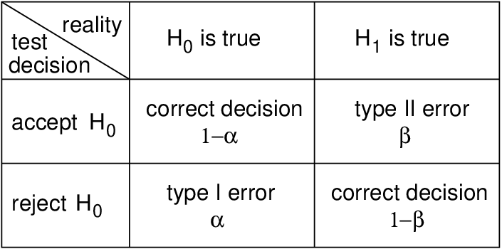
Indeed, in general the null hypothesis must be suitably formulated, such that it can be tested, i.e. such that the distribution function describing can be obtained, at least in principle. For example (A), since the test statistics is a sample mean, it is safe to assume a Gaussian distribution for : One can perform enough simulations rather easily, such that the central limit theorem applies. We use as null hypothesis the opposite of the formulated hypothesis (A). Nevertheless, it is impossible to calculate an acceptance interval for the Gaussian distribution based on the assumption that the mean is larger than a given value. Here, one can change the null hypothesis, such that instead an expectation value equal to is assumed. Hence, the null hypothesis assumes that the test statistics has a Gaussian distribution with expectation value . The variance of is unknown, but one can use, as for the calculation of error bars, the sample variance divided by . Now one calculates on this basis an interval with . Therefore, one rejects the null hypothesis if , which happens with probability . On the other hand, if the true expectation value is even larger than , then the probability of finding a mean with becomes even smaller than , i.e. less likely. Hence, the hypothesis (A) can be accepted or rejected on the basis of a fixed expectation value.
For a general hypothesis test, to evaluate the distribution of the test statistics , one can perform a Monte Carlo simulation. This means one draws repeatedly samples of size according to a distribution determined by the null hypothesis. Each time one calculates the test statistics and records a histogram of these values (or a sample distribution function ) which is an approximation of . In this way, the corresponding statistical information can be obtained. To save computing time, in most cases no Monte Carlo simulations are performed, but some knowledge is used to calculate or approximate .
In the following sections, the cases corresponding to examples (B), (C), (D) are discussed in detail. This means, it is explained how one can test for equality of discrete distributions via the chi-squared test and for equality of continuous distributions via the KS test. Finally, some methods for testing concerning (in-)dependence of data and for quantifying the degree of dependence are stated.
7.5.1 Chi-squared test
The chi-squared test is a method to compare histograms and discrete probability distributions. The test works also for discretized (also called binned) continuous probability distributions, where the probabilities are obtained by integrating the pdf over the different bins. The test comes in two variants:
- •
Either you want to compare the histogram for bins (see Sec. 7.3.3) describing the sample …, to a given discrete or discretized probability mass function with probabilities . The null hypothesis H0 is: “the sample follows a distribution given by ”.
Note that the probabilities are fixed and independent of the data sample. If the probabilities are parametrized and the parameter is determined by the sample (e.g. by the mean of the data) such that the probabilities fit the data best, related methods as described in Sec. 7.6.2 have to be applied.
- •
Alternatively, you want to compare two histograms obtained from two different samples …, and …, defined for the same bins . The null hypothesis H0 is: “the two samples follow the same distribution”.1313 13 Note that here we assume that the two samples have the same size, which is usually easy to achieve in simulations. A different case occurs when also the number of sample points is a random variable, hence a difference in the number of sample points makes the acceptance of H0 less likely, see [Press et al. (1995)].
In case the test is used to compare intrinsically discrete data, the intervals can conveniently be chosen such that each possible outcome corresponds to one interval. Note that due to the binning process, the test can be applied to high-dimensional data as well, where the sample is a set of vectors. Also non-numerical data can be binned. In these cases each bin represents either a subset of the high-dimensional space or, in general, a subset of the possible outcomes. For simplicity, we restrict ourselves here to one-dimensional numerical samples.
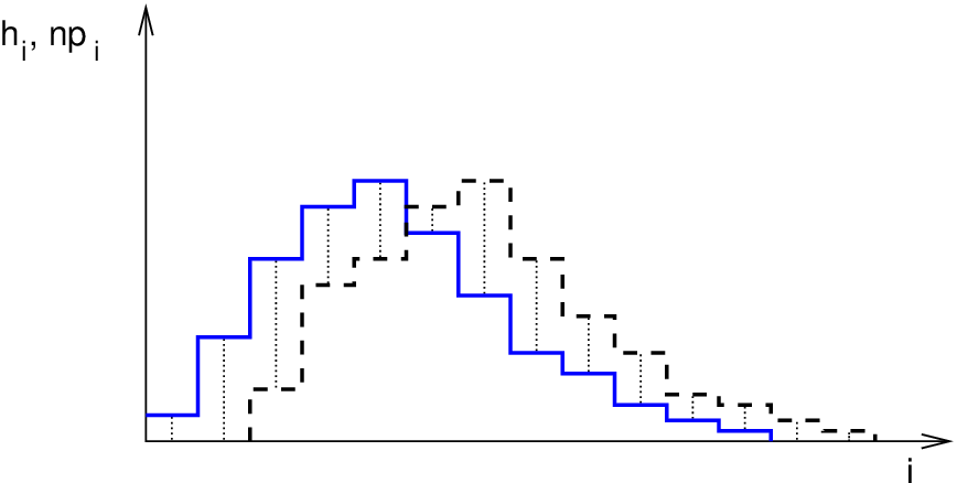
We start with the first case, where a sample histogram is compared to a probability distribution, corresponding to example (C) on page (B). The test statistics, called , is defined as:
| (7.68) |
with being the expected number of sample points in bin . The prime at the sum symbol indicates that bins with are omitted. The number of contributing bins is denoted by . If the pmf is nonzero for an infinite number of bins, the sum is truncated for terms . This means that the number of contributing bins will be always finite. Note that bins exhibiting but are not omitted. This results in an infinite value of , which is reasonable, because for data with but , the data cannot be described by the probabilities .
The chi-squared distribution with degrees of freedom (see Eq. (7.45)) describes the chi-squared test statistics, if the number of bins and the number of bin entries is large. The term in the number of degrees of freedom comes from the fact that the total number of data points is equal to the total number of expected data points , hence the different summands are not statistically independent. The probability density of the chi-squared distribution is given in Eq. (7.45). To perform the actual test, it is recommended to use the implementation in the GNU scientific library (GSL) (see Sec. ).
Next, a C function chi2_hd()
is shown which calculates the cumulative probability
(p-value) that
a value of or larger is obtained,
given the null hypothesis that the
GET SOURCE CODE
DIR:
randomness
FILE(S): chi2.c
sample was
generated
using the probabilities .
Arguments of chi2_hd()
are the number of bins, and two arrays h[] and p[]
containing the histogram and the probabilities , respectively:
double chi2_hd(int n_bins, int *h, double *p)
{
  int n;                      /* total number of sample points */
  double chi2;                                  /* chi^2 value */
  int K_prime;                  /* number of contributing bins */
  int i;                                            /* counter */

  n = 0;
  for(i=0; i<n_bins; i++)
    n += h[i];      /* calculate total number of sample_points */

  chi2 = 0.0; K_prime = 0;
  for(i=0; i<n_bins; i++)                   /* calculate chi^2 */
  {
    if(p[i] > 0)
    {
      chi2 += (h[i]-n*p[i])*(h[i]/(n*p[i])-1.0);
      K_prime ++;
    }
    else if(h[i] >0)       /* bin entry for zero probability ? */
    {
      chi2 = 1e60;
      K_prime ++;
    }
  }
  return(gsl_cdf_chisq_Q(chi2, K_prime-1));
}
First, in lines 8–10, the total number of sample points
is obtained from summing up all histogram entries. In the main loop,
lines 12–25, the value of is calculated. In parallel,
the number of contributing bins is determined. Finally (line 26)
the p-value is obtained using the GSL function
gsl_cdf_chisq_Q(). This p-value can be compared with
the significance level . If the the p-value is larger, the
null hypothesis is accepted, otherwise rejected.
Note that the result for the p-value clearly depends on the number of bins, and, if applicable, on the actual choice of bins. Nevertheless, all reasonable choices, although maybe leading to somehow different numerical results, will lead to the same decisions concerning the null hypothesis in most cases.
Next, we consider the case, where we want to compare two histograms corresponding to example (B) on page (B). In this case the statistics reads
| (7.69) |
The sum runs over all bins where or , and being the corresponding number of contributing bins. Consequently, the bins which should be included are uniquely defined, in contrast to the case where a histogram is compared to a distribution defined for infinitely many outcomes. Note that in the denominator the sum of the bin entries occurs, not the average. The reason is that the chi-squared distribution is a sum of standard Gaussian distributed numbers (variance 1) and here, where the differences of two (approximately) Gaussian quantities are taken, the resulting variance is the sum of the individual variances, approximated roughly by the histogram entries. To calculate the p-value, again the chi-squared distribution with degrees of freedom is to be applied. Here, no C implementation is shown, rather we refer the reader to exercise (6).
7.5.2 Kolmogorov-Smirnov test
Next, we consider the case where the statistical properties of a sample …, , obtained from a repeated experiment using a continuous random variable, is to be compared to a given distribution function . One could, in principle, compare a histogram and a correspondingly binned probability distribution using the chi-squared test explained in the previous section. Unfortunately, the binning is artificial and has an influence on the results (imagine few very large bins). Consequently, the method presented in this section is usually preferred, since it requires no binning. Note that if the distribution function is parametrized and if the parameter is determined by the sample (e.g. by the mean of the data) such that the fits the data best, the methods from Sec. 7.6.2 have to be applied.
The basic idea of the Kolmogorov-Smirnov test is to compare the distribution function to the empirical sample distribution function defined in Eq. (7.65). Note that is piecewise constant with jumps of size at the positions (assuming that each data point is contained uniquely in the sample).
Here again, one has several choices for the test statistics. For instance, one could calculate the area between and . Instead, usually just the maximum difference between the two functions is used:
| (7.70) |
Since the sample distribution function changes only at the sample points, one has to perform the comparison just before and just after the jumps. Thus, Eq. (7.70) is equivalent to
This sample statistics is visualized in Fig. 7.26.

The p-value, i.e. the probability of a value of as measured () or worse, given the null hypothesis that the sample is drawn from , is approximately given by (see [Press et al. (1995)] and references therein):
| (7.71) |
This approximation is already quite good for . Here, the following auxiliary probability function is used:
| (7.72) |
GET SOURCE CODE
DIR: randomness
FILE(S): ks.c
with and .
This function can be implemented most easily by a direct summation
[Press et al. (1995)]. The function Q_ks()
receives the value of
as argument and returns :
double Q_ks(double lambda)
{
  const double eps1 = 0.0001;  /* relative margin for stop */
  const double eps2 = 1e-10;   /* relative margin for stop */
  int i;                                   /* loop counter */
  double sum;                               /* final value */
  double factor;            /* constant factor in exponent */
  double sign;                               /* of summand */
  double term, last_term;        /* summands, last summand */

  sum = 0.0; last_term = 0.0; sign = 1.0;    /* initialize */
  factor = -2.0*lambda*lambda;
  for(i=1; i<100; i++)                           /* sum up */
  {
    term = sign*exp(factor*i*i);
    sum += term;
    if( (fabs(term) <= eps1*fabs(last_term)) ||
        (fabs(term) <= eps2*sum))
      return(2*sum);
    sign =- sign;
    last_term = term;
  }
  return(1.0);                /* in case of no convergence */
}
The summation (lines 13–22) is performed for at most 100 iterations. If the current term is small compared to the previous one or very small compared to the sum obtained so far, the summation is stopped (line 17–18). If this does not happen within 100 iterations, the sum has not converged (which means is very small) and is returned.
This leads to the following C implementation for the KS test. The
function ks() expects as arguments the number of sample points
n, the sample x[] and a pointer F
to the distribution function:
double ks(int n, double *x, double (*F)(double))
{
  double d, d_max;                    /* (maximum) distance */
  int i;                                    /* loop counter */
  double F_X;            /* empirical distribution function */

  qsort(x, n, sizeof(double), compare_double);

  F_X = 0; d_max = 0.0;
  for(i=0; i<n; i++)                    /* scan through F_X */
  {
    d = fabs(F_X-F(x[i]));   /* distance before jump of F_X */
    if( d> d_max)
      d_max = d;
    F_X += 1.0/n;
    d = fabs(F_X-F(x[i]));    /* distance after jump of F_X */
    if( d> d_max)
      d_max = d;
  }
  return(Q_ks( d_max*(sqrt(n)+0.12+0.11/sqrt(n))));
}
First the sample is sorted (line 7). This allows for a simple implementation of the sample distribution function, because at each sample data point, in the order of occurrence, the value of is increased by . When obtaining the maximum distance (lines 10–19), one has to compare to the distribution function just before (lines 12–14) and after (lines 15–18) the jumps. Note that this implementation works also for samples, where some data points occur multiple times.
For the actual test, one calculates the p-value for the given sample
using ks(). If the p-value exceeds the indented significance
level , the null hypothesis is accepted, i.e. the data is compatible with the distribution with high probability.
Usually quite small significances are used, e.g. .
This means that even substantial values of are accepted. Thus,
one rejects the null hypothesis only, as usual, in case the
probability for an error of type I is quite small.
It is also possible to compare two samples of sizes
via the KS test. The test
statistics for the two sample distribution functions is again
the maximum distance. The probability to find a value of
as obtained or worse, given the null hypothesis
that the samples
are drawn from the same distribution, is as above in Eq. (7.71), only one has to replace by the
“effective” sample size ,
for details see [Press et al. (1995)] and references therein.
It is straightforward to implement this test when using
the C function ks() shown above as template.
7.5.3 Statistical (in-)dependence
Here, we consider samples, which consist of pairs () of data points. Generalizations to higher-dimensional data is straightforward. The question is, whether the values depend on the values (or vice versa). In this case, one also says that they are statistically related. If yes, this means that if we know one of the two values, we can predict the other one with higher accuracy. The formal definition of statistical (in-) dependence was given in Sec. 7.1. An example of statistical dependence occurs in weather simulations: The amount of snowfall is statistically related to the temperature: If it is too warm or too cold, it will not snow. This also shows, that the dependence of two variables it not necessarily monotonous. In case one is interested in monotonous and even linear dependence, one usually says that the variables are correlated, see below.


GET SOURCE CODE
DIR: randomness
FILE(S): points0A.dat
points0B.dat
points1A.dat
points1B.dat
It is important to realize that we have to distinguish between statistical significance of a statistical dependence and the strength of the dependence. Say that our test tells us that the values are statistically related with high probability. This usually just means that we have a large sample. On the other hand, the strength of the statistical dependence can be still small. It could be, for eaxample, that a given value for will influence the probability distribution for only slightly. One the other hand, the strength can be large, which means, for example, knowing almost determines . But if we have only few samples points, we cannot be very sure whether the data points are related or not. Nevertheless, there is some connection: the larger the strength, the easier it is to show that the dependence is significant. For illustration consider a sample where the numbers are generated from a standard Gaussian distribution (expectation value 0, variance 1), while each number is drawn from a Gaussian distribution with expectation value (variance 1).1414 14 This is an example, where the random variables which described the sample are not identical. Hence, if , the data points are independent. Scatter plots, where each sample point () is shown as dot in the plane are exposed in Fig. 7.27. Four possibilities are presented, combined with . Below, we will also present what the methods we use here will tell us about these data sets.
In this section, first a variant of the chi-squared test is presented, which enables us to check whether data is independent. Next, the linear correlation coefficient is given, which states the strength of linear correlation. Finally, it is discussed how one can quantify the dependence within a sample, for example between sample points .
To test statistical dependence for a sample …, , one considers usually the null hypothesis: H “The sample points and the sample points are independent.” To test H0 one puts the pairs of sample points into two-dimensional histograms . The counter receives a count, if for data point we have and , for suitably determined bins and . Let and the number of bins in and direction, respectively. Next, one calculates single-value (or one-dimensional) histograms and defined by
| (7.73) |
These one-dimensional histograms describe how many counts in a certain bin arise for one variable, regardless of the value of the other variable. It is assumed that all entries of these histograms are not empty. If not, the bins should be adjusted accordingly. Note that holds.
Relative frequencies, which are estimates of probabilities, are obtained by normalizing with , i.e. and . If the two variables are independent, then the relative frequency to obtain a pair of values in bins and should be the product of the single-value relative frequencies. Consequently, by multiplying with one obtains the corresponding expected number of counts, under the assumption that H0 holds:
| (7.74) |
These expected numbers are compared to the actual numbers in the two-dimensional histogram via the test statistics, comparable to Eq. (7.68):
| (7.75) |
The statistical interpretation of is again provided by the chi-squared distribution. The number of degrees of freedom is determined by the number of bins () in the two-dimensional histogram minus the number of constraints. The constraints are given by Eq. (7.73), except that the total number of counts being is contained twice, resulting in . Consequently, the number of degrees of freedom is
| (7.76) |
Therefore, under the assumption that the and sample points are independent, gives the probability (p-value) of observing a test statistics of or larger. is here the distribution function of the chi-square distribution, see Eq. (7.45). This p-value has to be compared to the significance level . If , the null hypothesis is rejected.
GET SOURCE CODE
DIR: randomness
FILE(S): chi2indep.c
The following C function implements the chi-squared independence test
chi2_indep(). It receives the number of bins
in and direction as arguments, as well as a two-dimensional array,
which carries the histogram:
double chi2_indep(int n_x, int n_y, int **h)
{
  int n;                      /* total number of sample points */
  double chi2;                                  /* chi^2 value */
  int k_x, k_y;                 /* number of contributing bins */
  int k, l;                                        /* counters */
  int *hx, *hy;                  /* one-dimensional histograms */

  hx = (int *) malloc(n_x*sizeof(int));            /* allocate */
  hy = (int *) malloc(n_y*sizeof(int));

  n = 0;            /* calculate total number of sample_points */
  for(k=0; k<n_x; k++)
    for(l=0; l<n_y; l++)
      n += h[k][l];

  k_x = 0;                  /* calculate 1-dim histogram for x */
  for(k=0; k<n_x; k++)
  {
    hx[k] = 0;
    for(l=0; l<n_y; l++)
      hx[k] += h[k][l];
    if(hx[k] > 0)                   /* does x bin contribute ? */
      k_x++;
  }
  k_y = 0;                  /* calculate 1-dim histogram for y */
  for(l=0; l<n_y; l++)
  {
    hy[l] = 0;
    for(k=0; k<n_x; k++)
      hy[l] += h[k][l];
    if(hy[l] > 0)                   /* does y bin contribute ? */
      k_y++;
  }

  chi2 = 0.0;
  for(k=0; k<n_x; k++)                      /* calculate chi^2 */
    for(l=0; l<n_y; l++)
      if( (hx[k] != 0)&&(hy[l] != 0) )
        chi2 += pow(h[k][l]-(double) hx[k]*hy[l]/n, 2.0)/
          ((double) hx[k]*hy[l]/n);

  free(hx);
  free(hy);
  return(gsl_cdf_chisq_Q(chi2, k_x*k_y - k_x -k_y + 1));
}
First, the one-dimensional histograms are allocated (lines 9–10).
Then the total number of counts, i.e. the sample size, is calculated
(lines 12–15). In lines 17–26, the one-dimensional histogram for
the direction is obtained. Also the effective number of bins
in that direction is calculated. In lines 27–35, the same happens
for the direction. The actual value of the test
statistics is determined in lines 37–42. Finally,
the allocated memory is freed (lines 44-45) and the p-value
calculated (line 46), again the GSL function
gsl_cdf_chisq_Q() is used.
The p-values for the sample sets shown in Fig. 7.27 are as follows: , , , . Hence, the null hypothesis of independence would not be rejected (say ) for the case , which is actually correlated. On the other hand, if the number of samples is large enough, there is no doubt.
Once it is established that a sample contains dependent data, one can try to measure the strength of dependence. A standard way is to use the linear correlation coefficient (also called Pearson’s ) given by
| (7.77) |
This coefficient assumes, as indicated by the name, that a linear correlation exists within the data. The implementation using a C function is straight forward, see exercise (7). For the data shown in Fig. 7.27, the following correlation coefficients are obtained: , , , . Here, also in the two cases, where the statistics is low, the value of reflects whether or not the data is correlated. Nevertheless, this is only the case because we compare strongly correlated data to uncorrelated data. If we compare weakly but significantly correlated data, we will still get a small value of . Hence, to test for significance, it is better to use the hypothesis test based on the test statistics.
Finally, note that a different type of correlation may arise: So far it was always assumed that the different sample points (or sample vectors) are statistically independent of each other. Nevertheless, it could be the case, for instance, that the sample is generated using a Markov chain Monte Carlo simulation [Newman and Barkema (1999), Landau and Binder (2000), Robert and Casella (2004), Liu (2008)], where each data point is calculated using some random process, but also depends on the previous data point , hence is a kind of artificial sample time of the simulation. This dependence decreases with growing time distance between sample points. One way to see how quickly this dependence decreases is to use a variation of the correlation coefficient Eq. (7.77), i.e. a correlation function:
| (7.78) | |||||
The term will converge to for if it can be assumed that the distribution of the sample points is stationary, i.e. does not depend on the sample time. Therefore, is approximately , comparable to the nominator of the linear correlation coefficient Eq. (7.77). Usually one normalizes the correlation function by , which is just the sample variance in the stationary case, see Eq. (7.51):
| (7.79) |

Consequently, for any data, for example obtained from a Markov chain Monte Carlo simulation, will always hold, Then decreases with increasing difference , see for example Fig. 7.28. Very often the functional form is similar to an exponential . In theory, should converge to zero for , but due to the finite size of the sample, usually strong fluctuations appear for approaching . A typical time which measures how fast the dependence of the sample points decreases is given by , which is consistent with the above expression, if the correlation function decreases exponentially. At twice this distance, the correlation is already substantially decreases (to ). Consequently, if you want to obtain error bars for samples obtained from dependent data, you could include for instance only points in a sample, or just use instead of in any calculation of error bars. Although these error bars are different from those if the sample was really independent, it gives a fairly good impression of the statistical error.
Alternatively, to obtain a typical time without calculating a correlation function, you can also use the blocking method [Flyvbjerg (1998)]. Within this approach, you iteratively merge neighboring data points via and (iteration level corresponds to the original sample). You calculate the standard error bar for each iteration level. Once it reaches a plateau at level , the data is (almost) independent and the true error bar is given by the level value. Then is a typical time of independence of the data points.
If you are really just interested in error bars, i.e. you do not need to know the value of , you could also use the bootstrap approach which is not susceptible to dependence of data, see Sec. 7.3.4.
7.6 General estimators
In Sec. 7.3, different methods are presented of how to estimate parameters which can be obtained directly and simply from the given sample …, . In this section, a general method is considered which enables estimators to be obtained for arbitrary parameters of probability distributions. The method is based on the maximum-likelihood principle, which is exposed in Sec. 7.6.1. This principle can be extended to the modeling of data, where often a sample of triplets …, is given. Typically the data points represent some control parameter, which can be chosen in the simulation, such as the temperature of a gas. It is assumed that all values are different. Consequently, the simulation has been carried out at different values of the control parameter. The data points are averages of measurements (e.g. the density of the gas) obtained in the simulations for the fixed value of the control parameter. The values are the corresponding error bars.1515 15 Sometimes also the data points are measured quantities which are also characterized by error bars. The generalization of the methods to this case is straightforward. Modeling the data means that one wants to determine a relationship . Usually some assumptions or knowledge about the relationship are available, which means one has available one parametrized test function . Consequently, the set of parameters has to be adjusted such that the function fits the sample “best”. This is called data fitting and will be explained in Sec. 7.6.2. This approach can also be used to compare several fitted test functions to determined which represents the most suitable model.
7.6.1 Maximum likelihood
Here, we consider the following task: For a given sample …, and a probability distribution represented by a pmf or a pdf , we want to determine the parameters such that the pmf or pdf represents the data “best”. This is written in parentheses, because there is not unique definition what “best” means, or even a mathematical way to derive a suitable criterion. If one assumes no prior knowledge about the parameters, one can use the following principle:
Definition The maximum-likelihood principle states that the parameters should be chosen such that the likelihood of the data set, given the parameters, is maximal.
In case of a discrete random variable, if it can be assumed that the different data points are independent, the likelihood of the data is just given by the product of the single data point probabilities. This defines the likelihood function
| (7.80) |
For the continuous case, the probability to obtain during a random experiment exactly a certain sample is zero. Nevertheless, for a small uncertainty parameter , the probability to obtain a value in the interval is . Since enters just as a factor, it is not relevant to determining the maximum. Consequently, for the continuous case, one considers the following likelihood function
| (7.81) |
To find the maximum of a likelihood function analytically, one has to calculate the first derivatives with respect to all parameters, respectively, and requires them to be zero. Since calculating the derivative of a product involves the application of the product rule, it is usually more convenient to consider the log-likelihood function
| (7.82) |
This turns the product of single-data-points pmfs or pdfs into a sum, where the derivatives are easier to obtain. Furthermore, since the logarithm is a monotonous function, the maximum of the likelihood function is the same as the maximum of the log-likelihood function. Hence, the parameters which suit “best” are determined within the maximum-likelihood approach by the set of equations
| (7.83) |
Note that the fact that the first derivatives are zero only assures that an extremal point is obtained. Furthermore, these equations often have several solutions. Therefore, one has to check explicitly which solutions are indeed maxima, and which is the largest one. Note that maximum-likelihood estimators, since they are functions of the samples, are also random variables .
As a toy example, we consider the exponential distribution with the pdf given by Eq. (7.39). It has one parameter . The log-likelihood function for a sample …, is in this case
Taking the derivative with respect to we obtain:
This implies . It is easy to verify that this corresponds to a maximum. Since the expectation value for the exponential distribution is just , this is compatible with the result from Sec. 7.3, where it was shown that the sample mean is an unbiased estimator of the expectation value.
If one applies the maximum-likelihood principle to a Gaussian distribution with parameters and , one obtains (not shown here, see for example [Dekking et al (2005)]) as maximum-likelihood estimators the sample mean (for ) and the sample variance (for ), respectively. This means (see Eq. (7.54)) that the maximum-likelihood estimator for is biased. Fortunately, we know that the bias disappears asymptotically for . Indeed, it can be shown, under rather mild conditions on the underlying distributions, that all maximum-likelihood estimators for a parameter are asymptotically unbiased, i.e.
| (7.84) |
In contrast to the exponential and Gaussian cases, for many applications the maximum-likelihood parameter is not directly related to a standard sample estimator. Furthermore, can often even not be determined analytically. In this case, one has to optimize the log-likelihood function numerically, for example, using the corresponding methods from the GNU scientific library (GSL) (see Sec. ).
GET SOURCE CODE
DIR: randomness
FILE(S): max_likely.c
As example, we consider Fisher-Tippett distribution,
see Eq. (7.43), shifted to exhibit the maximum
at instead of at 0. Hence, we have two parameters and
to adjust. The function to be optimized (the target function),
i.e. the
log-likelihood function here, must be of a special format when using
the minimization functions of the
GSL. This first argument of the target function
contains the pdf parameters to be adjusted, i.e. the main argument vector of the target function.
This argument must be of the
type gsl_vector, which is a GSL type for vectors.
One needs to include <gsl/gsl_vector.h> to use this data type.
These vectors are created using gsl_vector_alloc(),
set elements via gsl_vector_set(), access elements via
gsl_vector_get() and delete the vectors via gsl_vector_free().
The usage of these functions should be self-explanatory from the
examples below, but you may also have a look at
the GSL documentation [Galassi et al. (2006)].
The second argument of the target function contains one pointer to all additional data needed to calculate the target function, i.e. the sample in this case. Thus, the sample must be stored in one chunk of memory. For this purpose, we use the following structure type:
typedef struct
{
  int       n;       /* number of sample points; */
  double   *x;                         /* sample */
}
sample_t;
Since the GSL package contains actually minimization functions, while we are interested in a maximum, the actual log-likelihood function returns minus the log-likelihood. The log-likelihood function reads as follows:
double ll_ft(const gsl_vector *par, void *param)
{
  double lambda, x0;                     /* parameters of pdf */
  sample_t *sample;                                 /* sample */
  double sum;          /* sum of log-likelihood contributions */
  int i;                                      /* loop counter */

  lambda = gsl_vector_get(par, 0);                /* get data */
  x0 = gsl_vector_get(par, 1);
  sample = (sample_t *) param;

  sum = sample->n*log(lambda);    /* calculate log likelihood */
  for(i=0; i<sample->n; i++)
    sum -= lambda*(sample->x[i]-x0) +
           exp(-lambda*(sample->x[i]-x0));

  return(-sum);                    /* return - log likelihood */
}
First, we convert the pointers passed as arguments to the data format that we find useful (lines 8–10). Next, the actual log likelihood
is calculated in lines 12–15 and finally returned with inverted sign (line 17).
The GSL has built in several minimization algorithms. They are
all put under one of two frameworks. One framework is for algorithms
which require the target function and its first derivatives.
The other framwork contains
algorithms where just the target function is sufficient.
Here we use the simplex algorithm,
which belongs to the latter form. It works by spanning a
simplex,1616
16
A simplex is a convex set in an -dimensional space
generated by corner points.
evaluating the target functions at the corners of the simplex,
and iteratively changing
the simplex until it is very small and contains the solution. Note that
the algorithm is only able to find local minima, and only one of them.
If several minima exist, the choice of the initial parameters
strongly influence the final results; Here, one maybe has to try several
parameters. For details see [Galassi et al. (2006)].
Here we only show how to use the minimizer. The minimizer itself
is stored in a special data structure of type
gsl_multimin_fminimizer. The target function
has to be put into a
“surrounding” variable of type gsl_multimin_function.
Furthermore, one needs two gsl_vector variables to store
the current estimate for the optimum (specifying the position of the simplex)
and to store the size of the simplex. Also, par is used here to
state the dimension of the target function argument (2) and
sample to store the sample.
These variables are declared as follows:
  int num_par;                        /* number of parameters */
  sample_t sample;                                  /* sample */

  gsl_multimin_fminimizer *s;           /* the full mimimizer */
  gsl_vector *simplex_size;        /* (relative) simplex size */
  gsl_vector *par; /* params to be optimized = args of target */
  gsl_multimin_function f;  /* holds function to be optimized */
The actual allocation and initialization of these variables may look as follows:
  sample.n = 10000;                          /* initilization */
  sample.x = (double *) malloc(sample.n*sizeof(double));
  num_par = 2;

  f.f = &ll_ft;                    /* initialize minimization */
  f.n = num_par;
  f.params = &sample;
  simplex_size = gsl_vector_alloc(num_par);  /* alloc simplex */
  gsl_vector_set_all(simplex_size, 1.0);      /* init simplex */
  par = gsl_vector_alloc(num_par);  /* alloc + init arguments */
  gsl_vector_set(par, 0, 1.0);
  gsl_vector_set(par, 1, 1.0);
  s =
    gsl_multimin_fminimizer_alloc(gsl_multimin_fminimizer_nmsimplex,
                                  num_par);
  gsl_multimin_fminimizer_set(s, &f, par, simplex_size);
The set-up of the minimizer object comes in two steps,
first allocation using gsl_multimin_fminimizer_alloc(),
then initialization via gsl_multimin_fminimizer_set()
while passing the target function, the starting point par
and the (initial) simplex size.1717
17
The simplex is spanned
by par and the vectors given by par plus (
simplex_size[i], ) for .
The sample.x[] array has to be filled with the actual
sample (not shown here).
The minimization loop looks as follows:
  do                                  /* perform minimization */
  {
    iter++;
    status = gsl_multimin_fminimizer_iterate(s);  /* one step */
    if(status)    /* error ? */
      break;
    size = gsl_multimin_fminimizer_size(s);    /* converged ? */
    status = gsl_multimin_test_size(size, 1e-4);
  }
  while( (status == GSL_CONTINUE) && (iter<100) );
The main work is done in gsl_multimin_fminimizer_iterate().
Then it is checked whether an error has occurred. Next,
the size of the simplex is calculated and finally tested
whether the size falls below some limit, here.
The actual estimate of the parameters can be obtained
via gsl_vector_get(s->x, 0) and gsl_vector_get(s->x, 1).
Note that finally all allocated memory should be freed:
  gsl_vector_free(par);                    /* free everything */
  gsl_vector_free(simplex_size);
  gsl_multimin_fminimizer_free(s);
  free(sample.x);
As an example, data points were generated according to a Fisher-Tippett distribution with parameters , . With the above starting parameters, the minimization converged to the values and after 39 iterations.
7.6.2 Data fitting
In the previous section, the parameters of a probability distribution are chosen such that the distribution describes the data best. Here, we consider a more general case, called modeling of data. As explained above, here a sample of triplets …, is given. Typically, the are measured values obtained from a simulation with some control parameter (e.g. the temperature) fixed at different values ; is the corresponding error bar of . Here, one wants to determine parameters such that the given parametrized function fits the data “best”, one says one wants to fit the function to the data. Similar to the case of fitting a pmf or a pdf, there is no general principle of what “best” means.
Let us assume that the are random variables, i.e. comparing different simulations. Thus, the measured values are scattered around their “true” values . This scattering can be described approximately by a Gaussian distribution with mean and variance :
| (7.85) |
This assumption is often valid, e.g. when each sample point is itself a sample mean obtained from a simulation performed at control parameter value , and is the corresponding error bar. The log-likelihood function for the full data sample is
Maximizing is equivalent to minimizing , hence one minimizes the mean-squared difference
| (7.86) |
This means the parameters are determined such that function follows the data points as close as possible, where the deviations are measured in terms of the error bars . Hence, data points with smaller error bar enter with more weight. The full procedure is called least-squares fitting.
The minimized mean-squared difference is a random variable. Note that the different terms are not statistically independent, since they are related by the parameters which are determined via minimizing . As a consequence, the distribution of is approximately given by chi-squared distribution (see Eq. (7.45) for the pdf) with degrees of freedom. This distribution can be used to evaluate the statistical significance of a least-squares fit, see below.
In case, one wants to model the underlying distribution function for a sample as in Sec. 7.6.1, say for a continuous distribution, it is possible in principle to use the least-squares approach as well. In this case one would fit the parametrized pdf to a histogram pdf, which has also the above mentioned sample format . Nevertheless, although the least-squares principle is derived using the maximum-likelihood principle, usually different parameters are obtained if one fits a pdf to a histogram pdf compared to obtaining these parameters from a direct maximum-likelihood approach. Often [Bauke (2007)], the maximum-likelihood method gives more accurate results. Therefore, one should use a least-squares fit mainly for a fit of a non-pmf/non-pdf function to a data set.
Fortunately, to actually perform least-squares fitting, you do not have to write your own fitting functions, because there are very good fitting implementations readily available. Both programs presented in Sec. 7.4, gnuplot and xmgrace, offer fitting to arbitrary functions. It is advisable to use gnuplot, since it offers higher flexibility for that purpose and gives you more information useful to estimate the quality of a fit.
As an example, let us suppose that you want to fit an algebraic function of the form to the data set of the file sg_e0_L.dat shown on page 7.4.1. First, you have to define the function and supply some rough (non-zero) estimations for the unknown parameters. Note that the exponential operator is denoted by ** and the standard argument for a function definition is x, but this depends only on your choice:
gnuplot> f(x)=e+a*x**b
gnuplot> e=-1.8
gnuplot> a=1
gnuplot> b=-1
The actual fit is performed via the fit command. The program uses the nonlinear least-squares Levenberg-Marquardt algorithm [Press et al. (1995)], which allows a fit data to almost all arbitrary functions. To issue the command, you have to state the fit function, the data set and the parameters which are to be adjusted. First, we consider the case where just two columns of the data are used or available (in this case, gnuplot assumes ). For our example you enter:
gnuplot> fit f(x) "sg_e0_L.dat" via e,a,b
Then gnuplot writes log information to the output describing the fitting process. After the fit has converged it prints for the given example:
After 17 iterations the fit converged.
final sum of squares of residuals : 7.55104e-06
rel. change during last iteration : -2.42172e-09

degrees of freedom (ndf) : 5
rms of residuals      (stdfit) = sqrt(WSSR/ndf)      : 0.00122891
variance of residuals (reduced chisquare) = WSSR/ndf : 1.51021e-06

Final set of parameters            Asymptotic Standard Error
=======================            ==========================

e               = -1.78786         +/- 0.0008548    (0.04781%)
a               = 2.5425           +/- 0.2282       (8.976%)
b               = -2.80103         +/- 0.08265      (2.951%)


correlation matrix of the fit parameters:

               e      a      b
e               1.000
a               0.708  1.000
b              -0.766 -0.991  1.000
The most interesting lines are those where the results
for your
parameters along with the standard error bar
are printed.1818
18
These “error bars” are calculated in a way
which is in fact correct only when fitting linear functions; hence,
they have to be taken with care. Additionally, the quality
of the fit can be estimated by the information provided in the three
lines beginning with “degree of freedom’’.
The first of these lines
states the number of degrees of freedom, which is just .
The mean-squared difference
is denoted as WSSR in the gnuplot
output. A measure of quality of the fit
is the probability
that the value of the mean-squared difference
is equal or larger compared to the value from the current fit, given the
assumption that the data points are distributed as in
Eq. (7.85)
[Press et al. (1995)].
The larger the value of
, the better is the quality of the fit.
As mentioned above, can be evaluated from a chi-squared
distribution with degrees of freedom.
To calculate using the gnuplot output
you can use the little program Q.c
#include <stdio.h>
#include <stdlib.h>
#include <math.h>
#include <gsl/gsl_cdf.h>

int main(int argc, char *argv[])
{
  double WSSRndf;
  int ndf;

  if(argc != 3)
  {
    printf("USAGE %s <ndf> <WSSR/ndf>\n", argv[0]);
    exit(1);
  }
  ndf = atoi(argv[1]);
  sscanf(argv[2], "%lf", &WSSRndf);
  printf("# Q=%e\n", gsl_cdf_chisq_Q(ndf*WSSRndf, ndf));

  return(0);
}
which uses the gsl_cdf_chisq_Q() function from the GSL (see Sec. ). The program is called in the form Q <ndf> <WSSR/ndf>, which can be taken from the gnuplot output. Note that in this case we obtain , which is so large, because was used, see below.
To watch the result of the fit along with the original data, just enter
gnuplot> plot "sg_e0_L.dat" w e, f(x)
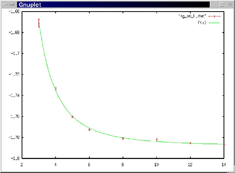
The result is displayed in Fig. 7.29.
Please note that the
convergence depends on the initial choice of the parameters. The
algorithm may be trapped into a local minimum in case the parameters
are too far away from the best values. Try the initial values
e=1, a=-3 and b=1!
Furthermore, not all function parameters have to be subjected to
the fitting. Alternatively, you can set some parameters to fixed
values and omit them from the via list at the end of the fit
command. Remember that
in the above example all data points enter into the
result with the same weight, i.e. is assumed.
You can tell the algorithm to consider
the error bars, for example supplied in the third column,
by typing
gnuplot> fit f(x) "sg_e0_L.dat" using 1:2:3 via e,a,b
Then, data points with larger error bars have less influence on the results. In this case a different result whith smaller value of will arise (try it !).
Finally, you can also restrict the data points which are considered for the fit, which is applicable if only a subset of the sample follows the function law you are considering. This can be done in the same way as restricting the range of plotted values, for instance using
gnuplot> fit [5:12] f(x) "sg_e0_L.dat" using 1:2:3 via e,a,b
More information on how to use the fit command, such as fitting higher-dimensional data, can be obtained when using the gnuplot online help via entering help fit.
Exercises
(solutions: see CD enclosed with book)
- 1.
Sampling from discrete distribution
Design, implement and test a function, which returns a random number which is distributed according to some discrete distribution function stored in an array
F, as describe in Sec. 7.2.2.SOLUTION SOURCE CODE DIR: randomness FILE(S): poisson.c
The function prototype reads as follows:
/******************** rand_discrete() *****************/
/** Returns natural random number distributed        **/
/** according a discrete distribution given by the   **/
/** distribution function in array ’F’               **/
/** Uses search in array to generate number          **/
/** PARAMETERS: (*)= return-paramter                 **/
/**       n: number of entries in array              **/
/**       F: array with distribution function        **/
/** RETURNS:                                         **/
/**     random number                                **/
/******************************************************/
int rand_discrete(int n, double *F)
For simplicity, you can use the
drand48()function from the standard C library to generate random numbers distributed according to .Furthermore, design, implement and test a function, which allocates and initializes the array
Ffor a Poisson distribution with parameter , see Eq. (7.27) for the probability mass function. The function should determine automatically how many entries ofFare needed, depending on the paramater . The function prototype reads as follows:/********************* init_poisson() *****************/ /** Generates array with distribution function **/ /** for Poisson distribution with mean mu: **/ /** p(k)=mu^k*exp(-mu)/x! **/ /** The size of the array is automatically adjusted. **/ /** PARAMETERS: (*)= return-paramter **/ /** (*) n_p: p. to number of entries in table **/ /** mu: parameter of distribution **/ /** RETURNS: **/ /** pointer to array with distribution function **/ /******************************************************/ double *init_poisson(int *n_p, double mu)
Hints: To determine the array sizes, you can first loop over the probabilities and take the first value
k_0wherek_0within the precision of the numerics. This value ofk_0serves as array size. Alternatively, you start with some size and extend the array if needed by doubling its size. For testing purposes, you can generate many numbers, calculate the mean and compare it with . Alternatively, you could record a histogram (see Chap. ) and compare with Eq. (7.27). - 2.
Inversion Method for Fisher-Tippett distribution
Design, implement and test a function, which returns a random number which is distributed according to the Fisher-Tippett distribution Eq. (7.43) with parameter . Use the inversion method.
SOLUTION SOURCE CODE DIR: randomness FILE(S): fischer_tippett.c
The function prototype reads as follows:
/******************** rand_fisher_tippett() ***********/
/** Returns random number which is distributed       **/
/** according the Fisher-Tippett distribution        **/
/** PARAMETERS: (*)= return-paramter                 **/
/**       lambda: parameter of distribution          **/
/** RETURNS:                                         **/
/**     random number                                **/
/******************************************************/
double rand_fisher_tippett(double lambda)
Remarks: For simplicity, you can use the
drand48()function from the standard C library to generate random numbers distributed according to . To test your function, you can calculate the mean of the generated numbers, for instance, and compare it with the expectation value . - 3.
Variance of data sample
Design, implement and test a function, which calculates the variance of a sample of data points. Use directly Eq. (7.51), i.e. do not use an equivalent form of Eq. (7.21), since this form is more susceptible to rounding errors.
SOLUTION SOURCE CODE DIR: randomness FILE(S): variance.c
The function prototype reads as follows:
/********************** variance() ********************/
/** Calculates the variance of n data points         **/
/** PARAMETERS: (*)= return-paramter                 **/
/**        n: number of data points                  **/
/**        x: array with data                        **/
/** RETURNS:                                         **/
/**     variance                                     **/
/******************************************************/
double variance(int n, double *x)
Remark: The so-called corrected double-pass algorithm [Chan et al. (1983)] aims at further reducing the rounding error. It is based on the equation
The second would be zero for exact arithmetic and accounts for rounding erros occurring in the second term. It becomes important in particular if the expectation value is large. Perform experiments for generating Gaussian distributed number with and , without and with the correction.
- 4.
Bootstrap
Design, implement and test a function, which uses bootstrapping to calculate the confidence interval at significance level given in Eq. (7.66).
SOLUTION SOURCE CODE DIR: randomness FILE(S): bootstrap_ci.c
The function prototype reads as follows:
/***************** bootstrap_ci() *********************/
/** Calculates a confidence interval by ’n_resample’ **/
/** times resampling the given sample points         **/
/** and each time evaluation the estimator ’f’       **/
/** PARAMETERS: (*)= return-paramter                 **/
/**           n: number of data points               **/
/**           x: array with data                     **/
/**  n_resample: number of bootstrap iterations      **/
/**       alpha: confidence level                    **/
/**           f: function (pointer) = estimator      **/
/**     (*) low: (p. to) lower boundary of conf. int.**/
/**    (*) high: (p. to) upper boundary of conf. int.**/
/** RETURNS:                                         **/
/**     (nothing)                                    **/
/******************************************************/
void bootstrap_ci(int n, double *x, int n_resample,
                  double alpha, double (*f)(int, double *),
                  double *low, double *high)
Hints: Use the function
bootstrap_variance()as example. To get the entries at the positions defined via Eq. (7.66), you can sort the bootstrap sample first usingqsort(), see Sec. .You can test your function by using the provided main file
bootstrap_test.c, the auxiliary filesmean.candvariance.cand by compiling withcc -o bt bootstrap_test.c bootstrap_ci.c mean.c -lm -DSOLUTION. Note that the macro definition-DSOLUTIONmakes themain()function to callbootstrap_ci()instead ofbootstrap_variance(). - 5.
Plotting data
Plot the data file
FTpdf.datusing xmgrace. The file contains a histogram pdf generated for the Fisher-Tippett distribution. The file format is 1st column: bin number, 2nd: bin midpoint, 3rd: pdf value, 4th: error bar. UseSOLUTION SOURCE CODE DIR: randomness FILE(S): FTplot.agr
the “block data” format to read the files (columns 2,3,4). Create a plot with inset. The main plot should show the histogram pdf with error bars and logarithmically scaled axis, the inset should show the data with linear axes. Describe the plot using a text label placed in the plot. Choose label sizes, line width and other styles suitably. Store the result as
.agrfile and export it to a postscript (eps) file.The result should look similar to:
![[Uncaptioned image]](0910.4545v1/FTplot.png)
- 6.
Chi-squared test
Design, implement and test a function, which calculates the test statistics for two histograms according Eq. (7.69). The function should return the p-value, i.e. the
SOLUTION SOURCE CODE DIR: randomness FILE(S): chi2hh.c
cumulative probability (‘‘p-value’’) that a value of or larger is obtained under the assumption that the two histograms were obtained by sampling from the same (discrete) random variable.
The function prototype reads as follows:
/********************* chi2_hh() ***********************/
/** For chi^2 test: comparison of two histograms      **/
/** to probabilities: Probability to                  **/
/** obtain the corresponding  chi2 value or worse.    **/
/** It is assumed that the total number of data points**/
/*+ in the two histograms is equal !                  **/
/**                                                   **/
/** Parameters: (*) = return parameter                **/
/**  n_bins: number of bins                           **/
/**       h: array of histogram values                **/
/**      h2: 2nd array of histogram values            **/
/**                                                   **/
/** Returns:                                          **/
/**       p-value                                     **/
/*******************************************************/
double chi2_hh(int n_bins, int *h, int *h2)
Hints: Use the functio
chi2_hd()as example. Include a test, which verifies that the total number of counts in the two histograms agree.To test the function: Generate two histograms according to a binomial distribution with parameters
par_nand 0.5 orpar_p. Perform a loop for different values ofpar_pand calculate the p-value each time using thegsl_cdf_chisq_Q()function of the GNU scientific library (GSL) (see Sec. ). - 7.
Linear correlation coefficient
Design, implement and test a function, which calculates the linear correlation coefficient to measure the strength of a correlation for a sample …, .
SOLUTION SOURCE CODE DIR: randomness FILE(S): lcc.c
The function prototype reads as follows:
/**************************** lcc() ********************/
/** Calculates the linear correlation coefficient     **/
/**                                                   **/
/** Parameters: (*) = return parameter                **/
/**     n: number of data points                      **/
/**     x: first element of sample set                **/
/**     y: second element of sample set               **/
/**                                                   **/
/** Returns:                                          **/
/**       r                                           **/
/*******************************************************/
double lcc(int n, double *x, double *y)
Remark: Write a
main()function which generates a sample in the following way: the numbers are generated from a standard Gaussian distribution while each number is drawn from a Gaussian distribution with expectation value (variance 1). Study the result for different values of and . - 8.
Least-squares fitting
Copy the program from exercise (2) to a new program and change it such that numbers for a shifted Fisher-Tippett with parameters and peak position are generated. The numbers should be stored in a histogram and a histogram pdf should be written to the standard output.
SOLUTION SOURCE CODE DIR: randomness FILE(S): fitFT.gp
fisher_tippett2.c- •
Choose the histogram parameters (range, bin range) such that the histograms match the generated data well.
- •
Run the program to generate numbers for parameters and . Pipe the histogram pdf to a file (e.g. using
> ft.datat the end of the call). - •
Plot the result using gnuplot.
- •
Define the pdf for the Fisher-Tippett distribution in gnuplot and fit the function to the data with and as adjustable parameters. Choose a suitable range for the fit.
- •
Plot the data together with the fitted function.
- •
How does the result compare to the maximum-likelihood fit presented in Sec. 7.6.1?
- •
Does the fit (in particular for ) get better if you increase the number of sample points to ?
Hints: The shift is implemented by just adding to the generated random number. Use either the histograms from Chap. , or implement a “poor-mans histogram” via an array
hist( see also in themain()function of thereject.cprogram partly presented in Sec. 7.2.4). - •
Bibliography
- [Abramson and Yung (1986)] Abramson, B. and Yung, M. (1986). Construction through decomposition: a divide-and-conquer algorithm for the N-queens problem, CM ’86: Proceedings of 1986 ACM Fall joint computer conference, pp. 620–628. (IEEE Computer Society Press, Los Alamitos)
- [Abramson and Yung (1989)] Abramson, B. and Yung, M. (1989). Divide and conquer under global constraints: A solution to the N-queens problem, Journal of Parallel and Distributed Computing 6, pp. 649–662.
- [Aho et al. (1974)] Aho, A. V., Hopcroft, J. E., and Ullman, J. D. (1974). The Design and Analysis of Computer Algorithms, (Addison-Wesley, Reading (MA)).
- [Albert and Barabási (2002)] Albert, R. and Barabási, A.-L. (2002). Statistical mechanics of complex networks, Rev. Mod. Phys. 74, pp. 47–97.
- [Allen and Tildesley (1989)] Allen, M. P., and Tildesley, D. J. (1989). Computer Simulation of Liquids, (Oxford University Press, Oxford).
- [Alta Vista]
Alta Vista, search engine, see
http://www.altavista.com/. - [APS]
APS, American Physical Society, journals see
http://publish.aps.org/. - [arXiv]
arXiv, preprint server,
see
http://arxiv.org/. - [Bauke (2007)] Bauke, H. (2007). Parameter estimation for power-law distributions by maximum likelihood methods, Eur. Phys. J. B 58, pp. 167–173.
- [Beamer]
Beamer class, a LaTeX package; written by Till Tantau, see
http://latex-beamer.sourceforge.net/. - [Becker (2007)] Becker, P. (2007). The C++ Standard Library Extensions, (Addison-Wesley Longman, Amsterdam).
- [Binder (1981)] Binder, K. (1981). Finite size scaling analysis of ising model block distribution functions, Z. Phys. B 43, pp. 119–140.
- [Binder and Heermann (1988)] Binder, K. and Heermann, D. W. (1988). Monte Carlo Simulations in Statistical Physics, (Springer, Heidelberg).
- [Bolobas (1998)] Bolobas, B. (1998). Modern Graph Theory, (Springer, New York).
- [Boost]
boost collection of libraries; available, including documentation,
at
http://www.boost.org/. - [Cardy (1996)] Cardy, J. (1996). Scaling and Renormalization in Statistical Physics, (Cambridge University Press, Cambridge).
- [Chan et al. (1983)] Chan, T. F., Golub, G.H., and LeVeque, R. J. (1983). Algorithm for Computing the Sample Variance: Analysis and Recommendations, Amer. Statist. 37, pp. 242–247.
- [Claiborne (1990)] Claiborne, J. D. (1990). Mathematical Preliminaries for Computer Networking, (Wiley, New York).
- [Comp. Sci. Eng. (2008)] Computational Provenance, special issue of Computing in Science & Engineering 10 (3), pp. 3–52.
- [Cormen et al. (2001)] Cormen, T. H., Clifford, S., Leiserson, C. E., and Rivest, R. L. (2001). Introduction to Algorithms, (MIT Press).
- [CTAN]
Comprehensive TeX Archive Network:
http://www.ctan.org/. - [Dekking et al (2005)] Dekking, F. M., Kraaikamp, C., Lopuhaä, H. P., and Meester, L. E. (2005). A Modern Introduction to Probability and Statistics, (Springer, London).
- [Devroye (1986)] Devroye, L. (1986). Non-Uniform Random Variate Generation, (Springer, London).
- [Dhar (2001)] Dhar, A. (2001). Heat Conduction in a One-dimensional Gas of Elastically Colliding Particles of Unequal Masses, Phys. Rev. Lett. 86, pp. 3554–3557.
- [Marsaglia]
“Diehard” test provided by George Marsaglia,
see source code at
http://www.stat.fsu.edu/pub/diehard/. - [Efron (1979)] Efron, B. (1979). Bootstrap methods: another look at the jacknife, Ann. Statist. 7, pp. 1–26.
- [Efron and Tibshirani (1994)] Efron, B. and Tibshirani, R. J. (1994). An Introduction to the Bootstrap, (Chapman & Hall/CRC, Boca Raton).
- [Fernandez and Criado (1999)] Fernandez, J. F. and Criado, C. (1999). Algorithm for normal random numbers, Phys. Rev. E 60, pp. 3361–3365.
- [Ferrenberg et al. (1992)] Ferrenberg, A. M., Landau, D. P. and Wong, Y. J. (1992). Monte Carlo Simulations: Hidden Errors from “Good” Random Number Generators, Phys. Rev. Lett. 69, pp. 3382–3384.
- [Flyvbjerg (1998)] Flyvbjerg, H. (1998). Error Estimates on Averages of Correlated Data, in: Kertész, J. and Kondor, I. (Eds.), Advances in Computer Simulation, (Springer, Heidelberg), pp. 88–103.
- [Galassi et al. (2006)]
Galassi M. et al (2006). GNU Scientific Library Reference Manual, (Network Theory Ltd, Bristol),
see also
http://www.gnu.org/software/gsl/. - [Ghezzi et al. (1991)] Ghezzi C., Jazayeri, M. and Mandrioli, D. (1991). Fundamentals of Software Engineering, (Prentice Hall, London).
- [Google]
Google search engine,
see
http://www.google.com/. - [GraphViz]
GraphViz graph drawing package, see
http://www.graphviz.org/. - [Grassberger et al. (2002)] Grassberger, P., Nadler, W. and Yang, L. (2002). Heat conduction and entropy production in a one-dimensional hard-particle gas, Phys. Rev. Lett. 89, 180601, pp. 1–4.
- [Haile (1992)] Haile, J. M. (1992). Molecular Dynamics Simulations: Elementary Methods, (Wiley, New York).
- [Hartmann (1999)] Hartmann, A. K. (1999). Ground-state behavior of the 3d J random-bond Ising model, Phys. Rev. B 59, pp. 3617–3623.
- [Hartmann and Rieger (2001)] Hartmann, A. K. and Rieger, H. (2001). Optimization Algorithms in Physics, (Wiley-VCH, Weinheim).
- [Heck (1996)] Heck, A. (1996). Introduction to Maple, (Springer, New York).
- [Hotbits]
HotBits webpage: here you
can order files with random numbers which are generated
from radioactive decay, see
http://www.fourmilab.ch/hotbits/. - [Hucht (2003)]
Hucht, A. (2003). The program fsscale,
see
http://www.thp.uni-duisburg.de/fsscale/. - [INSPEC]
INSPEC, literature data base,
see
http://www.inspec.org/publish/inspec/. - [JAVA]
JAVA programming language, see
http://www.java.com/. - [Johnsonbaugh and Kalin (1994)] Johnsonbaugh, R. and Kalin, M. (1994). Object Oriented Programming in C++, (Macmillan, London).
- [Josuttis (1999)] Josuttis, N. M. (1999). The Standard C++ Library, (Addison-Wesley, Boston).
- [Karlsson (2005)] Karlsson, B. (2005). Beyond the C++ Standard Library. An Introduction to Boost, (Addison-Wesley Longman, Amsterdam).
- [Kernighan and Pike (1999)] Kernighan, B. W. and Pike, R. (1999). The Practice of Programming, (Addisin-Wesley, Boston).
- [Kernighan and Ritchie (1988)] Kernighan, B. W. and Ritchie, D. M. (1988). The C Programming Language, (Prentice Hall, London).
- [Lamport and Bibby (1994)] Lamport, L. and Bibby, D. (1994). LaTeX : A Documentation Preparation System User’s Guide and Reference Manual, (Addison Wesley, Reading (MA)).
- [Landau and Binder (2000)] Landau, D.P. and Binder, K. (2000). A Guide to Monte Carlo Simulations in Statistical Physics, (Cambridge University Press, Cambridge (UK)).
- [Lefebvre (2006)] Lefebvre L. (2006). Applied Probability and Statistics, (Springer, New York).
- [Lewis and Papadimitriou (1981)] Lewis, H. R. and Papadimitriou, C. H. (1981). Elements of the Theory of Computation, (Prentice Hall, London).
- [Liu (2008)] Lui, J. S. (2008). Monte Carlo Strategies in Scientific Computing, (Springer, Heidelberg).
- [Loukides and Oram (1996)]
Loukides, M. and Oram, A. (1996). Programming with GNU Software, (O’Reilly, London);
see also
http://www.gnu.org/manual. - [Lüscher (1994)] Lüscher, M. (1994). A portable high-quality random number generator for lattice field-theory simulations, Comput. Phys. Commun. 79, pp. 100–110.
- [Lyx]
Lyx, document processor based on LaTeX, see
http://www.lyx.org/. - [Matsumoto and Nishimura (1998)] Matsumoto, M. and Nishimura, T. (1998). Mersenne twister: a 623-dimensionally equidistributed uniform pseudo-random number generator, ACM Transactions on Modeling and Computer Simulation 8, pp. 3–30.
- [Mehlhorn and Näher (1999)]
Mehlhorn, K. and Näher, St. (1999).
The LEDA Platform of Combinatorial and Geometric Computing
(Cambridge University Press, Cambridge);
see also
http://www.mpi-sb.mpg.de/LEDA/leda.html. - [Meyers (2005)] Meyers, S. (2005). Effective C++: 55 Specific Ways to Improve Your Programs and Designs, (Addison-Wesley, Reading (MA)).
- [Morgan (1984)] Morgan, B. J. T. (1987). Elements of Simulation, (Cambridge University Press, Cambridge).
- [Newman and Barkema (1999)] Newman, M. E. J. and Barkema, G. T. (1999). Monte Carlo Methods in Statistical Physics, (Clarendon Press, Oxford).
- [Newman (2003)] Newman, M. E. J. (2003) The Structure and Function of Complex Networks, SIAM Review 45, pp. 167–256.
- [Newman et al. (2006)] Newman, M. E. J., Barabasi, A.-L., and Watts, D. (2006). The Structure and Dynamics of Networks, ( Princeton University Press, Princeton).
- [Philipps (1987)]
Phillips, J. (1987) .
The Nag Library: A Beginner’s Guide
(Oxford University Press, Oxford);
see also
http://www.nag.com. - [Oram and Talbott (1991)] Oram, A. and Talbott, S. (1991). Managing Projects With Make, (O’Reilly, London).
- [PhysNet]
PhysNet, the Physics Departments and
Documents Network, see
http://physnet.uni-oldenburg.de/PhysNet/physnet.html. - [Press et al. (1995)] Press, W. H., Teukolsky, S. A., Vetterling, W. T., and Flannery, B. P. (1995). Numerical Recipes in C, (Cambridge University Press, Cambridge).
- [Povray]
Povray,
Persistence of Vision raytracer, see
http://www.povray.org/. - [Qantis]
Quantis: A hardware true random number
generator. It is based on the quantum mechanical process of photon
scattering. It can be connected to a computer
via USB port or PCI slot. More information can be found at
http://www.idquantique.com/products/quantis.htm. - [R]
R is a software package for statistical computing,
freely avalaible at
http://www.r-project.org/. - [Rapaport (1995)] Rapaport, D. C. (1995). The Art of Molecular Dynamics Simulations, (Cambridge University Press, Cambridge).
- [Robert and Casella (2004)] Robert, C. P. and Casella, G. (2004). Monte Carlo Statistical Methods, (Springer, Berlin)
- [Robinson and Torrens (1974)] Robinson, M. T. and Torrens, I. M. (1974). Computer simulation of atomic displacement cascades in solids in the binary collision approximation, Phys. Rev. B 9, pp. 5008–5024.
- [Romeo]
Romeo, a database for publisher copyright policies and self-archiving,
see
http://www.sherpa.ac.uk/romeo/. - [Rumbaugh et al. (1991)] Rumbaugh, J., Blaha, M., Premerlani, W. , Eddy, F., and Lorensen, W. (1991). Object-Oriented Modeling and Design, (Prentice Hall, London).
- [Scott (1979)] Scott, D. W. (1979). On optimal and data-based histograms, Biometrica 66, pp. 605–610.
- [Sedgewick (1990)] Sedgewick, R., (1990). Algorithms in C, (Addison-Wesley, Reading (MA)).
- [Skansholm (1997)] Skansholm, J. (1997). C++ from the Beginning, (Addison-Wesley, Reading (MA)).
- [Sommerville (1989)] Sommerville, I. ( 1989). Software Engineering, (Addison-Wesley, Reading (MA)).
- [Sosic and Gu (1991)] Sosic, R. and Gu, J. (2001). Fast Search Algorithms for the N-Queens Problem, IEEE Trans. on Systems, Man, and Cybernetics 21, pp. 1572–1576.
- [STL]
Standard Template Library, see
http://www.sgi.com/tech/stl/download.html. - [Stroustrup (2000)] Stroustrup, B. (2000). The C++ Programming Language, (Addison-Wesley Longman, Amsterdam).
- [Sutter (1999)] Sutter, H. (1999). Exceptional C++: 47 Engineering Puzzles, Programming Problems, and Solutions, (Addison-Wesley Longman, Amsterdam).
- [SVN]
Subversion version control system, see
http://subversion.tigris.org/. - [Swamy Thulasiraman (1991)] Swamy, M. N. S. and Thulasiraman, K. (1991). Graphs, Networks and Algorithms, (Wiley, New York).
- [Texinfo]
Texinfo system, see
http://www.gnu.org. For some tools there is a texinfo file. To read it, call the editor ’emacs’ and type crtl+’h’ and then ’i’ to start the texinfo mode. - [TUG]
TUG, TeXUser Group, see
http://www.tug.org/. - [valgrind]
Valgrind memory checker; more information,
including a user manual,
can be obtained from
http://www.valgrind.org/. - [Vattulainen et al. (1994)] Vattulainen, I., Ala-Nissila, T. and Kankaala, K. (1994). Physica Test for Random Numbers in Simulations, Phys. Rev. Lett. 73, pp. 2513–2516.
- [Web of Science]
Web of Science, see
http://www.isiwebofknowledge.com/ - [Westphal]
Westphal Electronic
(
http://www.westphal-electronic.com/) sells divices which produce true random numbers based on thermal noise in Z diodes. They can be connected to a computer via USB port or bluetooth. - [Wikipedia]
Wikipedia is a free online encyclopedia, currently containing
more than 2.5 million articles,
see
http://www.wikipedia.org/. - [Wilson (2007)] Wilson, M. (2007). Extended STL, (Addison-Wesley Longman, Amsterdam).
- [xmgrace]
Xmgrace (X Motiv GRaphing,
Advanced Computation and Exploration of data), see
http://http://plasma-gate.weizmann.ac.il/Grace/. - [Yahoo]
Yahoo search engine,
see
http://www.yahoo.com/. - [Ziff (1998)] Ziff, R. M. (1998). Four-tap shift-register-sequence random-number generators, Computers in Physics 12, pp. 385–392.
- [zlib]
zlib compression library, see
http://www.zlib.net/.