We consider large $N$ Yang Mills theory with $D$ adjoint scalar fields in $d$ dimensions for $d=0$ or 1. We show the existence of a non-trivial saddle point of the functional integral at large $D$ which is characterized by a mass gap for the adjoint scalars. We integrate out the adjoint scalars in a $1/D$ expansion around the saddle point. In case of one dimension which is regarded as a circle, this procedure leads to an effective action for the Wilson line. We find an analogue of the confinement/deconfinement transition which consists of a second order phase transition from a uniform to a non-uniform eigenvalue distribution of the Wilson line, closely followed by a Gross-Witten-Wadia transition where a gap develops in the eigenvalue distribution. The phase transition can be regarded as a continuation of a Gregory-Laflamme transition. Our methods involve large values of the dimensionless ’tHooft coupling. The analysis in this paper is quantitatively supported by earlier numerical work for $D=9$ .

1 Introduction and Summary

Matrix models in low dimensions (especially 0 and 1) have served as useful tools in many contexts. These include (i) $c\leq 1$ matrix models, which correspond to non-critical string theories [1], (ii) large $N$ reduced models and their variants [2, 3], (iii) BFSS matrix theory, which corresponds to DLCQ of M-theory [4], (iv) IKKT matrix model of type IIB string theory [5, 6], (v) D0 brane black holes [7, 8, 9, 10, 11, 12, 13, 14], (vi) KK reduction of 4-dimensional ${\cal N}=4$ SYM on $S^{3}$ [15, 16, 17, 18], (vii) The BMN matrix model [19], (viii) the matrix model of unstable D0 branes [20, 21], (ix) D branes on tori [22, 23, 24, 25], etc. In many cases, one can regard these models as dimensional reduction of large $N$ Yang-Mills theories. In models arising from D branes, the YM theories are typically supersymmetric; however, in some situations the theory is effectively described by the bosonic sector. The obvious advantage of such a description, when it is possible, is that it is easily amenable to numerical calculations, and in some fortunate circumstances, to some powerful exact methods.

In this paper, we consider the following system for $d=0,1$ :

S=\frac{1}{g^{2}}\int d^{d}x{\rm Tr}\left(\frac{1}{2}\sum_{I=1}^{D}D_{\mu}Y^{I}D^{\mu}Y^{I}-\sum_{I,J}\frac{1}{4}[Y^{I},Y^{J}]^{2}\right),

(1.1)

where $D_{\mu}$ refers to the covariant derivative $\partial_{\mu}-i[A_{\mu},.]$ . $A_{\mu},Y^{I}$ are $SU(N)$ matrices. For $d=0$ there is no gauge field and the first term is absent. For $d=1$ , there is a single gauge field $A_{0}$ which is non-dynamical.

The action (1.1) can be regarded as a dimensional reduction of $D+d$ dimensional bosonic YM theory to $d$ dimensions. The specific physical context we have in mind in the present paper is related to case (ix) above, which is discussed in [22, 23, 24, 25] and reviewed below in Section 5.

In the $d=1$ case, we consider the dimension as a circle, of circumference $\beta$ , and study the partition function and other quantities as a function of $\beta$ . It was conjectured in [22, 23, 24, 25], on the basis of numerical investigations, that the $d=1$ system exhibits a phase transition which is analogous to the confinement/deconfinement transition of ${\cal N}=4$ SYM on $S^{3}$ . The phase transition was argued to be the weak coupling continuation of the black hole/black string transition of the $d=2$ model. One of the motivations for the present work was to understand the nature of the phase transition analytically.

Our results are briefly as follows:

1.

In the limit of large $D$ , the model (1.1) has a non-trivial saddle point characterized by a non-zero value of $\langle{\rm Tr}Y^{I}Y^{I}\rangle$ . The large $D$ scaling is defined by keeping a modified ’tHooft coupling $\tilde{\lambda}=\lambda D$ fixed.
2.

In this limit, fluctuations around the above saddle point are suppressed by powers of 1/ $D$ . This enables us to develop a systematic expansion, in $1/D$ , of the partition function and other quantities as a function of the radius of the circle.
3.

In the $d=0$ case, the exact partition function is calculable up to $1/D$ at finite $N$ (first shown in [6]), whereas in the $d=1$ case our results are obtained in the leading large $N$ limit.
4.

Since the condensate provides a dynamically generated mass to the adjoint scalars $Y_{I}$ , it is possible to explicitly integrate them out. In the $d=1$ case, this allows us to compute an effective action $S_{\rm eff}(W)$ for the Wilson line

$W=P\exp[i\int_{0}^{\beta}dtA_{0}]$ (1.2)

in a $1/D$ expansion.
5.

The $S_{\rm eff}$ computed in this fashion provides the first analytic evidence, in a $1/D$ expansion, for the phase transitions mentioned above. It confirms the appearance of a double transition¹¹ 1 We thank S. Minwalla for a discussion on this point.: (i) a second order phase transition characterized by the onset of non-uniformity in the eigenvalue distribution of $W$ , followed by (ii) a third order Gross-Witten-Wadia (GWW) transition signalling the appearance of a gapped phase [26, 27, 28]. The appearance of a double transition is supported by the numerical works in [24, 25]²² 2 We differ from [24, 25], though, regarding the order of the two transitions. See Section 4.3 for details.. The phase transition temperatures $T_{c1}$ and $T_{c2}$ , computed up to $1/D$ , show excellent agreement with their results in the $D=9$ case, as shown in the following table (see Section 4.3 for more details and other comparisons):

$T_{c1}$ $T_{c2}$

Our result 0.895 0.917

Numerical result 0.8761 0.905
6.

Our methods involve large values of the dimensionless ’tHooft coupling.

	$T_{c1}$	$T_{c2}$
Our result	0.895	0.917
Numerical result	0.8761	0.905

The large $D$ technique used in this paper for $d=0,1$ has earlier been used in [6] in the $d=0$ context. Our results for $d=0$ are in complete agreement with those of [6], though our method is slightly different (see Section 3 for details) in a way that enables a natural generalization to higher dimensions. A large $D$ expansion has also been used in certain lattice theories [29]. Our methods also have some overlap with that of [8, 9] where a series of self-consistent equations (gap equations) are introduced to determine various condensates and a GWW type transition is suggested.

The paper is organized as follows. In Section 2 we set up the main calculational method for the $d=1$ model. The method consists of introducing an $SO(D)$ -invariant dynamical field to get rid of the commutator-squared interaction. This leads to an action quadratic in the adjoint scalars with a dynamical mass term, which allows us to integrate them out. We work out the example of the $d=0$ model in Section 3 to test the method. We show the existence of a non-trivial saddle point in which a mass is generated for the adjoints. We explain the nature of the large $D$ limit and compute the partition function at finite $N$ in a $1/D$ expansion. In Section 4 we come back to the $d=1$ model to derive the effective action for the Wilson line in a $1/D$ expansion. We show the existence of a second order phase transition followed by a GWW transition. In Section 5 we provide a D brane realization of our model, following earlier work [22, 23, 24, 25] which we briefly review. In Section 6 we conclude with a discussion.

This paper arose as part of a larger project of exploring dynamical black hole/black string transitions in terms of a dynamical large $N$ transition in a unitary matrix model [30].

2 The $d=1$ model: preliminaries

We will set up the $d=1$ model in this section, test the formalism with the simpler case of $d=0$ in Section 3, and continue on to Section 4 to solve the $d=1$ model. A D brane realization of the $d=0,1$ models is discussed in Section 5.

It is convenient to rescale the adjoint scalars $Y^{I}$ in (1.1) to $gY^{I}$ , so that the action becomes

\displaystyle S

\displaystyle\kern-18.0pt=\int_{0}^{\beta}dt\,{\rm Tr}\left(\sum_{I=1}^{D}\frac{1}{2}\left(D_{0}Y^{I}\right)^{2}-\sum_{I,J}\frac{g^{2}}{4}[Y^{I},Y^{J}][Y^{I},Y^{J}]\right).

(2.1)

We have assumed the theory to be on a circle, of circumference $\beta$ , which can be interpreted either as a Euclidean time direction or as a spatial circle. The covariant derivative is defined by $D_{0}Y^{I}=\partial_{t}Y^{I}-i[A_{0},Y^{I}]$ .

The large $N$ limit is defined by keeping the ’tHooft coupling $\lambda=g^{2}N$ fixed, as $N\to\infty$ . It is convenient to define the following related dimensionless quantities

	$\displaystyle\beta_{\rm eff}$	$\displaystyle=\beta\lambda^{1/3}=\beta(g^{2}N)^{1/3},$		(2.2)
	$\displaystyle\lambda_{\rm eff}$	$\displaystyle=\lambda\beta^{3}=\beta_{\rm eff}^{3}.$		(2.3)

For later convenience it is useful here to summarise various alternative definitions of coupling constant which we will use in this paper in different contexts:

$\lambda$	’tHooft coupling	$g^{2}N$
$\tilde{g}^{2}$	’tHooft like coupling at large $D$ and finite $N$	$g^{2}D$
$\tilde{\lambda}$	’tHooft like coupling at large $D$ and large $N$	$\lambda D$
$\lambda_{\rm eff}$	dimensionless ’tHooft coupling	$\lambda\beta^{3}$

The last line refers only to the $d=1$ case.

We would like to explore the partition function

Z=\int{\cal D}A_{0}{\cal D}Y^{I}e^{-S},

(2.4)

as a function of $\beta_{\rm eff}$ . We will also be interested in the effective action $S_{\rm eff}(A_{0})$ , defined by

\exp[-S_{\rm eff}(A_{0})]=\int{\cal D}Y^{I}e^{-S}.

(2.5)

It will turn out that $S_{\rm eff}$ depends only on the gauge-invariant content of the gauge potential, namely on the eigenvalues of the Wilson line $W$ (1.2).

The first step in solving the model consists of making the action (2.1) quadratic in the $Y^{I}$ by introducing an auxiliary field $B_{ab}$ . Let us write $Y^{I}=\sum_{a=1}^{N^{2}-1}Y_{a}^{I}\lambda_{a}$ , where $\lambda_{a}$ are the generators of $SU(N)$ . This leads to an expression

-{\rm Tr}[Y^{I},Y^{J}][Y^{I},Y^{J}]=(Y^{I}_{a}Y^{I}_{b})M_{ab,cd}(Y_{c}^{J}Y_{d}^{J}),

(2.6)

which is written in terms of $SO(D)$ -invariant $Y$ -bilinears, where

\displaystyle M_{ab,cd}=-\frac{1}{4}\Bigl\{{\rm Tr}[\lambda_{a},\lambda_{c}][\lambda_{b},\lambda_{d}]+(a\leftrightarrow b)+(c\leftrightarrow d)+(a\leftrightarrow b,c\leftrightarrow d)\Bigr\}.

(2.7)

Properties of the matrix $M$ are discussed in detail in Appendix A. Using the fact that $M$ is invertible³³ 3 It might be puzzling, at first sight, that $M$ does not have a zero mode since (2.6) clearly vanishes for special configurations of the ‘ $Y^{I}$ ’s, e.g. when all ‘ $Y^{I}$ ’s commute. The resolution is that $M$ has both positive and negative eigenvalues (see (A.13)) and therefore has light-like vectors which, however, do not correspond to zero eigenvalues. We thank Toby Wiseman for a useful discussion on this point.⁴⁴ 4 The indefinite signature of $M$ (A.13) involves some subtlety in choosing the contour of the functional integral in (2.8). E.g. we need to choose real contours for components of $B_{ab}$ along the positive eigenspace of $M$ and purely imaginary contours otherwise. The correct choice ensures finiteness of the normalization constant ${\cal N}$ ., we can write

	$\displaystyle Z=$	$\displaystyle{\cal N}\int{\cal D}B{\cal D}A_{0}{\cal D}Y^{I}e^{-S(B,A_{0},Y)},$
	$\displaystyle S(B,A_{0},Y)$	$\displaystyle=\int_{0}^{\beta}dt\,\left[\frac{1}{2}\left(D_{0}Y^{I}_{a}\right)^{2}-i\frac{1}{2}B_{ab}Y_{a}^{I}Y_{b}^{I}+\frac{1}{4g^{2}}B_{ab}M^{-1}_{ab,cd}B_{cd}\right],$		(2.8)

with the following classical equation of motion for $B_{ab}$ :

\frac{1}{g^{2}}M^{-1}_{ab,cd}B_{cd}=iY^{I}_{a}Y_{b}^{I}.

(2.9)

In the above $1/{\cal N}\equiv\int{\cal D}B\,\exp[-\int\ dt\,B_{ab}M^{-1}_{ab,cd}B_{cd}/(4g^{2})]$ , which we will ignore in the rest of the paper since it involves only a numerical factor. Since the action (2.8) is quadratic in $Y^{I}$ , we can formally integrate them out, to get

	$\displaystyle Z=$	$\displaystyle\int{\cal D}B{\cal D}A_{0}e^{-S_{\rm eff}(B,A_{0})},$
	$\displaystyle S_{\rm eff}(B,A_{0})$	$\displaystyle=\int_{0}^{\beta}\kern-5.0ptdt\,\frac{1}{4g^{2}}B_{ab}M^{-1}_{ab,cd}B_{cd}+\frac{D}{2}\log{\rm det}\left((D_{0}^{2})_{ab}+iB_{ab}\right).$		(2.10)

For large $D$ ⁵⁵ 5 In much of this paper, we will treat $D$ as an arbitrarily specifiable parameter, except in the section dealing with comparison with D branes, where we put $D=9$ . The precise scaling at large $D$ is defined in Eqns. (3.6) and (3.12). See also comments at the end of Section 4.1.⁶⁶ 6 Although the large $N$ scaling is not apparent in (2.10), the action as well as the measure admits a topological expansion in powers of $1/N$ for fixed $\lambda$ , as is apparent from expressions such as (3.13). which scales as $1/g^{2}$ , we may expect the one-loop determinant to be comparable with the classical term in (2.10) and hence modify the naive classical solution $B_{ab}=0$ . We will assume, and shortly justify, that (2.10) admits a gauge-invariant time-independent solution, of the form (see, e.g. Eqns. (3.15) and (4.8))

\displaystyle\overline{B}_{ab}=i\triangle_{0}^{2}\delta_{ab}.

(2.11)

The appearance of ‘ $i$ ’ is due to the fact, as we will see later, that the solution corresponds to a saddle point in the complex plane. The condensate in terms of the original physical variables $Y^{I}$ , however, turns out to be real:

\displaystyle\langle{\rm Tr}Y^{I}Y^{I}\rangle=\frac{N}{2g^{2}}\triangle_{0}^{2},

(2.12)

where we have used (2.9), and also $M_{ab,cd}^{-1}\delta_{cd}=\frac{1}{2N}\delta_{ab}$ , which is derived in Eqn. (A.12).

To proceed, we write the $B_{ab}$ field as the sum of a constant trace piece and the rest, as

\displaystyle B_{ab}(t)=B_{0}\delta_{ab}+gb_{ab}(t).

(2.13)

where $b_{ab}(t)$ satisfies $\int dt\,b_{aa}(t)=0$ . We will show below that $B_{0}$ has a saddle point value of the form $\overline{B}_{0}=i\triangle_{0}^{2}$ , consistent with (2.11). Substituting (2.13) in the action in (2.8) we get⁷⁷ 7 Note the appearance of an effective mass term for the adjoint scalars $Y^{I}_{a}$ in the saddle point $\overline{B}_{0}=i\triangle_{0}^{2}$ . In [23] such a mass term is added by hand to integrate out the $Y^{I}$ ; here the mass term is dynamically generated.

\displaystyle Z

\displaystyle=\int dB_{0}\ {\cal D}A_{0}{\cal D}b_{ab}\ {\cal D}Y^{I}e^{-S},\quad S=S_{0}+S_{q}+S_{int},

(2.14)

where⁸⁸ 8 Strictly speaking, the last term in $S_{q}$ is a cubic term and should be regarded as an interaction. However, when we consider $B_{0}$ as an external parameter (unintegrated) we can regard this term as quadratic.,

$\displaystyle S_{0}$	$\displaystyle=\frac{\beta NB_{0}^{2}}{8g^{2}},$
$\displaystyle S_{q}$	$\displaystyle=\int_{0}^{\beta}dt\left(\frac{1}{4}b_{ab}M_{ab,cd}^{-1}b_{cd}+\frac{1}{2}\left(D_{0}Y_{a}^{I}\right)^{2}-\frac{i}{2}B_{0}Y^{I2}_{a}\right),$
$\displaystyle S_{int}$	$\displaystyle=-\int_{0}^{\beta}dt\left(\frac{ig}{2}b_{ab}Y^{I}_{a}Y^{I}_{b}\right).$	(2.15)

Before proceeding to solve this model, let us discuss the $d=0$ matrix model as a partial test of our formalism.

3 The $d=0$ model

The $d=0$ model is defined by a partition function⁹⁹ 9 Most of the results in this section are in [6] who have discussed this model earlier in the context of the IKKT matrix model. Our method, however, is slightly different, especially in the way we distinguish between the diagonal and the off-diagonal fluctuations of the auxiliary field $B_{ab}$ (see, e.g. (2.13) and (B.2)) which allows for a natural generalization to the $d=1$ model.

\displaystyle Z=\int dY^{I}\exp[-S],\quad S=-\frac{g^{2}}{4}{\rm Tr}\sum_{I,J}[Y^{I},Y^{J}]^{2}.

(3.1)

Here $Y^{I}$ are $SU(N)$ hermitian matrices which are normalized the same way as in (2.1). A D brane interpretation of this model is discussed in Section 5.

Like in the previous section for $d=1$ , we can rewrite (3.1) as

$\displaystyle Z$	$\displaystyle=\int dB_{0}db_{ab}dY^{I}\exp[-S],$	(3.2)
$\displaystyle S$	$\displaystyle=S_{0}+S_{q}+S_{int},$
$\displaystyle S_{0}$	$\displaystyle=\frac{NB_{0}^{2}}{8g^{2}},~~S_{q}=\frac{1}{4}b_{ab}{M}_{ab,cd}^{-1}b_{cd}-i\frac{B_{0}}{2}Y^{I2}_{a},~~S_{int}=-\frac{ig}{2}b_{ab}Y^{I}_{a}Y^{I}_{b}.$	(3.3)

Integrating out the $Y^{I}$ gives us the $d=0$ analogue of (2.10) where $B_{ab}$ is split into $B_{0}$ and $b_{ab}$ :

	$\displaystyle Z$	$\displaystyle=\int dB_{0}db_{ab}e^{-S_{\rm eff}(B_{0},b_{ab})},$
	$\displaystyle S_{\rm eff}(B_{0},b_{ab})$	$\displaystyle=\frac{NB_{0}^{2}}{8g^{2}}+\frac{1}{4}b_{ab}{M}^{-1}_{ab,cd}b_{cd}+\frac{D}{2}\log{\rm det}\left(iB_{0}\delta_{ab}+igb_{ab}\right).$		(3.4)

3.1 The large $D$ limit

Let us make a formal Taylor expansion of $S_{\rm eff}$ in powers of $b_{ab}$ :

$\displaystyle S_{\rm eff}(B_{0},b_{ab})$	$\displaystyle=S^{(0)}(B_{0})+\frac{1}{2}S^{(2)}_{ab;cd}(B_{0})b_{ab}b_{cd}+S_{\rm eff}^{int},$
$\displaystyle S^{(0)}(B_{0})$	$\displaystyle=\frac{NB_{0}^{2}}{8g^{2}}+\frac{D}{2}\log{\rm det}\left(iB_{0}\delta_{ab}\right),$
$\displaystyle S^{(2)}_{ab;cd}(B_{0})$	$\displaystyle=\frac{1}{2}M^{-1}_{ab,cd}+\frac{g^{2}D}{2}\frac{\partial^{2}\log{\rm det}\left(iB_{0}\delta_{rs}+i\bar{b}_{rs}\right)}{\partial\bar{b}_{ab}\partial\bar{b}_{cd}}\Bigr\|_{\bar{b}_{rs}=0},$
$\displaystyle S_{\rm eff}^{int}$	$\displaystyle=O(b^{3}),$	(3.5)

where in defining $S^{(2)}$ we have used $\bar{b}_{ab}\equiv gb_{ab}$ in order to exhibit the $g$ dependence explicitly. There is no linear term in the above Taylor expansion since $b_{aa}=0$ . Let us define a large $D$ limit by keeping

\displaystyle{\tilde{g}}^{2}\equiv g^{2}D,

(3.6)

fixed. It is easy to see that

\displaystyle S^{(0)}(B_{0})=O(D),\quad S^{(2)}_{ab;cd}(B_{0})=O(1),\quad S_{\rm eff}^{int}=O(1/D).

(3.7)

Let us now do the integral in (3.4) over $b_{ab}$ , to give

	$\displaystyle Z=$	$\displaystyle\int dB_{0}\exp[-{\cal S}(B_{0})],$		(3.8)
	$\displaystyle\frac{{\cal S}(B_{0})}{D}=$	$\displaystyle{\cal S}_{0}(B_{0},\tilde{g})+\frac{1}{D}{\cal S}_{1}(\tilde{g})+O\left(\frac{1}{D^{2}}\right),$		(3.9)

where

	$\displaystyle{\cal S}_{0}(B_{0},\tilde{g})$	$\displaystyle=\frac{1}{D}S^{(0)}(B_{0})=\frac{NB_{0}^{2}}{8{\tilde{g}}^{2}}+\frac{1}{2}\log{\rm det}\left(iB_{0}\delta_{ab}\right),$
	$\displaystyle{\cal S}_{1}(B_{0},\tilde{g})$	$\displaystyle=\frac{1}{2}\log{\rm det}S^{(2)}_{ab;cd}.$		(3.10)

The first ‘log det’ is essentially a 1-loop integral over $Y^{I}$ , while the second ‘log det’ is a 1-loop integral over $b_{ab}$ (see Figure 6(a) and (b)). In Appendix B we will present an explicit computation of these quantities. We find (see (B.7))

$\displaystyle{\cal S}_{0}(B_{0})$	$\displaystyle=\frac{NB_{0}^{2}}{8{{\tilde{g}}}^{2}}+\frac{(N^{2}-1)}{4}\log\left(-\frac{B_{0}^{2}}{{\tilde{g}}^{2}N}\right),$
$\displaystyle{\cal S}_{1}(B_{0})$	$\displaystyle=\frac{N^{2}-1}{2}\log\left(1-\frac{{\tilde{g}}^{2}N}{B_{0}^{2}}\right)+\frac{N^{2}(N+1)(N-3)}{8}\log\left(1-\frac{2{\tilde{g}}^{2}}{B_{0}^{2}}\right)$
	$\displaystyle+\frac{N^{2}(N-1)(N+3)}{8}\log\left(1+\frac{2{\tilde{g}}^{2}}{B_{0}^{2}}\right).$	(3.11)

In the $d=1$ case, an explicit finite $N$ , large $D$ result such as Eqn. (3.11) is difficult to obtain, but we will derive an analogue of Eqn. (3.14) below. Furthermore, as remarked at the end of Section 4.1, for $d=1$ we will not take the strict $D=\infty$ limit since criticality involves $1/D$ effects.

3.2 Large $D,N$ limit

It is easy to see that both ${\cal S}_{0}$ and ${\cal S}_{1}$ admit a ’tHooft-like expansion in which

\displaystyle\tilde{\lambda}=\lambda D=g^{2}ND={\tilde{g}}^{2}N,

(3.12)

is kept fixed. We obtain an expansion of the sort

\displaystyle\frac{{\cal S}}{DN^{2}}=\left({\cal S}_{0,0}+\frac{1}{N^{2}}{\cal S}_{0,1}+\cdots\right)+\frac{1}{D}\left({\cal S}_{1,0}+\frac{1}{N^{2}}{\cal S}_{1,1}+\cdots\right)+\cdots.

(3.13)

In the diagrammatic evaluation described in the Appendices, such an expansion indeed corresponds to a topological expansion. Explicitly, from (3.11), we get

	$\displaystyle\frac{\cal S}{DN^{2}}=$	$\displaystyle\frac{B_{0}^{2}}{8\tilde{\lambda}}+\frac{1}{4}\log\frac{-B_{0}^{2}}{\tilde{\lambda}}+\frac{1}{D}\left\{\frac{\tilde{\lambda}}{B_{0}^{2}}-\frac{1}{2}\left(\frac{\tilde{\lambda}}{B_{0}^{2}}\right)^{2}+\frac{1}{2}\log\left(1-\frac{\tilde{\lambda}}{B_{0}^{2}}\right)\right\}$
		$\displaystyle+O\left(1/D^{2}\right)+O\left(1/N^{2}\right).$		(3.14)

3.3 The saddle point

We are left with evaluating (3.8). Because of the appearance of an overall factor of $N^{2}$ in (3.14), we can evaluate (3.8) using a saddle point method (see a similar calculation presented in Appendix C in a toy example). The saddle point value is given by

\overline{B}_{0}=i\triangle_{0}^{2},\quad\triangle_{0}^{4}=2\tilde{\lambda}\left(1+\frac{7}{3D}\right)+O(1/D^{2}).

(3.15)

The same result is also derived in [6] in a slightly different manner. [6] also performed a numerical analysis which agrees with the above analytical calculation and also with the numerical calculations of [22, 23].

Using the above saddle point, we get the free energy,

\displaystyle F=-\frac{\log Z}{DN^{2}}=-\frac{1}{4}+\frac{\log 2}{4}+\frac{1}{D}\left(-\frac{5}{8}+\frac{1}{2}\log\frac{3}{2}\right)+O\left(\frac{1}{D^{2}}\right).

(3.16)

4 The $d=1$ model: result

After gaining some experience with the $d=0$ matrix model, we now return to the more involved case, the $d=1$ model. We start with (2.15), and as with Eqns. (3.8) and (B.2), we first integrate out the $Y^{I}$ and the $b_{ab}$ to obtain

\displaystyle Z=\int dB_{0}{\cal D}A_{0}e^{-{\cal S}(B_{0},A_{0})},

(4.1)

where

e^{-{\cal S}(B_{0},A_{0})}=\int{\cal D}b_{ab}{\cal D}Y^{I}e^{-S},

(4.2)

with $S$ defined as in (2.15). Different from the previous section, we consider large $N$ case only in this section.

It is convenient to parametrize $A_{0}$ by choosing a gauge in which $A_{0}$ is time-independent and is also diagonal: $A_{0ij}=\alpha_{i}\delta_{ij}$ . The gauge-invariant content of $A_{0}$ is then given by the moments

\displaystyle u_{n}=\frac{1}{N}{\rm Tr}W^{n}=\frac{1}{N}\sum_{i=1}^{N}e^{in\beta\alpha_{i}},

(4.3)

where $W$ is the Wilson loop operator, defined in (1.2). The above gauge fixing gives rise to a Faddeev Popov Jacobian (See [16])

\displaystyle{\cal D}A_{0}=\prod_{i}d\alpha_{i}e^{-S_{FP}},\quad S_{FP}=N^{2}\sum_{n}\frac{1}{n}|u_{n}|^{2}.

(4.4)

It is convenient to parametrize $B_{0}=i\triangle^{2}$ , since the saddle point value will be real in terms of $\triangle$ as in the $d=0$ case (3.15). From now on, we will denote ${\cal S}(B_{0},A_{0})$ as ${\cal S}(\triangle,\{u_{n}\})$ .

Note that there is a Jacobian involved in changing from the integration measure over the eigenvalues $\alpha_{i}$ to the integration measure over $u_{n},\bar{u}_{n}$ ; however, it is $O(N)$ and is hence subleading compared to the classical action which is $O(N^{2})$ [31]. Since in this section we will be concerned with the leading term in the $1/N$ expansion, we will ignore this Jacobian.

4.1 Computation of ${\cal S}(\triangle,\{u_{n}\})$ in leading large $D$

As in Section 3, we can ignore the interaction $S_{int}$ in the large $D$ limit. Hence the leading result of the effective action is obtained by integrating out the $Y^{I}$ from $S_{q}$ in (2.15).

We can integrate out $Y^{I}$ by using the propagator studied in Appendix D (following [16]) and obtain

\displaystyle\frac{D}{2}\log\left(\hbox{det}\left(-D_{0}^{2}+\triangle^{2}\right)\right)=

\displaystyle\frac{DN^{2}\beta\triangle}{2}-D\sum_{n=1}^{\infty}\frac{x^{n}}{n}|u_{n}|^{2}.

(4.5)

Here $x=e^{-\beta\triangle}$ and we have ignored $1/N$ terms and irrelevant constant terms. We also ignored a temperature dependent divergent term.

Combining the above equation with $S_{0}$ from (2.15), and adding the contribution from (4.4), we get

\displaystyle\frac{{\cal S}(\triangle,\{u_{n}\})}{DN^{2}}=-\frac{\beta\triangle^{4}}{8\tilde{\lambda}}+\frac{\beta\triangle}{2}+\sum_{n=1}^{\infty}\left(\frac{1/D-x^{n}}{n}\right)|u_{n}|^{2}.

(4.6)

The $1/D$ term comes from (4.4). The reason it is kept here is that near the critical temperature this term will turn out to be more significant than other $O(1/D)$ terms from $S_{int}$ which we will encounter in the next subsection.

Our task is to evaluate (4.1), with ${\cal S}(B_{0},A_{0})={\cal S}(\triangle,\{u_{n}\})$ given above. It is useful to first perform the integral over $B_{0}$ , using a saddle point method similar to Section 3. In other words, for fixed external $u_{n}$ , let us now solve the saddle point equation

\displaystyle-\frac{\triangle^{3}}{2\tilde{\lambda}}+\frac{1}{2}+\sum_{n=1}^{\infty}e^{-n\beta\triangle}|u_{n}|^{2}=0.

(4.7)

It is difficult to solve this equation for $\triangle(\{u_{n}\})$ exactly. However, for small $u_{n}$ , it is possible to solve it in a power series in the $u_{n}$ . This leads to the following saddle point solution

\displaystyle\triangle_{0}(\{u_{n}\})={\tilde{\lambda}}^{1/3}\left(1+\frac{2}{3}\sum_{n=1}^{\infty}{\bar{x}}^{n}|u_{n}|^{2}\right)+\cdots,

(4.8)

where

\displaystyle\bar{x}=\exp[-\beta{\tilde{\lambda}}^{1/3}].

(4.9)

Substituting (4.8) in (4.6), we get a Landau-Ginzburg type effective action for the $u_{n}$ :

$\displaystyle\frac{{\cal S}(\{u_{n}\})}{DN^{2}}$	$\displaystyle=\frac{3}{8}\beta{\tilde{\lambda}}^{1/3}+a_{1}\|u_{1}\|^{2}+b_{1}\|u_{1}\|^{4}+\sum_{n=2}^{\infty}a_{n}\|u_{n}\|^{2}+\cdots,$
$\displaystyle a_{n}$	$\displaystyle=\frac{1}{n}\left(1/D-{\bar{x}}^{n}\right),$
$\displaystyle b_{1}$	$\displaystyle=\frac{1}{3}\beta{\tilde{\lambda}}^{1/3}{\bar{x}}^{2},$	(4.10)

where the $\cdots$ involve other $u^{4}_{n}$ terms for $n>1$ , which are ignored for reasons stated below.

Let us analyze the phase structure of the theory by using (4.10) (see Figure 1).¹⁰¹⁰ 10 We will show below that inclusion of higher loop terms does not change the nature of phase transitions, although it changes the critical temperature and numerical values of various thermodynamical quantities. Our analysis will be similar to [16]. Note that for $\bar{x}<1/D$ all ‘ $a_{n}$ ’s are positive. This implies that $\{u_{n}=0$ $\forall$ $n=1,2,...\}$ is a minimum of the potential.¹¹¹¹ 11 The issue of whether it is a local or a global minimum is more subtle, and depends on details of higher order terms in (4.10). We will argue below that in a $1/D$ expansion the higher order terms can be ignored and $u_{n}=0$ is a global minimum.

Refer to caption — Figure 1: Phase transitions: ${\cal S}$ vs $|u_{1}|$ (see (4.10), (4.26)). As $T$ crosses $T_{c1}$ , $u_{1}$ becomes tachyonic and there is a second order phase transition which signals an onset of non-uniformity in the eigenvalue distribution $\rho(\alpha)$ . At $T=T_{c2}$ , characterized by a potential minimum at $|u_{1}|=1/2$ , a gap develops in the eigenvalue distribution, signalling a GWW transition.

Recall that $u_{1}=0={\rm Tr}W$ corresponds to an analog of the confinement phase in gauge theory. The vanishing of all $u_{n}$ also has a familiar interpretation. Let us define an eigenvalue density of the Wilson line (1.2) by

\displaystyle\rho(\alpha)=\frac{1}{N}\sum_{n=1}^{N}\delta(\alpha-\alpha_{i}).

(4.11)

In terms of this, the $u_{n}$ are given by

\displaystyle u_{n}=\int_{0}^{\frac{2\pi}{\beta}}d\alpha\rho(\alpha)e^{-in\beta\alpha}.

(4.12)

The vanishing of all $u_{n}$ therefore corresponds to a uniform eigenvalue distribution.

Let us now consider the effect of increasing the temperature, or equivalently increasing $\bar{x}$ . As $\bar{x}$ crosses $1/D$ , i.e. $T$ crosses a critical temperature given by

\displaystyle T_{c1}=\frac{{\tilde{\lambda}}^{1/3}}{\log D}={\lambda^{1/3}}\frac{D^{1/3}}{\log D},

(4.13)

the sign of $a_{1}$ in (4.10) flips, while the coefficient of $|u_{1}|^{4}$ and the coefficients of all $|u_{n}|^{2},n>1$ remains positive. The ‘ $|u_{n}|$ ’s remain zero for $n>1$ ¹²¹² 12 Because of couplings such as $u_{-2}u_{1}^{2}$ discussed in Section 4.2, higher $u_{n}$ ’s pick up some non-zero values at higher orders in $1/D$ . However, these can be ignored in the present discussion. whereas $|u_{1}|$ assumes a small non-zero value

\displaystyle\langle|u_{1}|\rangle=\sqrt{-\frac{a_{1}}{2b_{1}}}=\sqrt{\frac{(3D\log D)\delta T}{2{\tilde{\lambda}}^{1/3}}}-\frac{3}{8}\sqrt{6D}\left(\log D\right)^{5/2}\left(\frac{\delta T}{\tilde{\lambda}^{1/3}}\right)^{5/2}+\cdots,

(4.14)

at $T=T_{c1}+\delta T$ for small and positive $\delta T$ . ¹³¹³ 13 $\delta T$ here is assumed to be small enough such that $\langle|u_{1}|\rangle$ satisfies the bound $|u_{1}|\leq 1/2$ discussed below.

The order of the phase transition can be determined by studying the free energy. It is easy to show that, for small $\delta T$ , the Landau Ginzburg free energy is of the form

\displaystyle{\cal S}/(DN^{2})={\rm constant}+{\rm constant}(\delta T)^{2}\Theta(\delta T)+O\left(\frac{1}{D},\frac{1}{N^{2}}\right).

(4.15)

The second derivative of the above function with respect to $\delta T$ is discontinuous at $\delta T=0$ . Thus we have a second order phase transition. We should remark that the transition is characteristic of the large $N$ limit and is expected to be smoothened at finite $N$ , as has been argued in [16].

As we increase the temperature further, we encounter another phase transition. To understand this phase transition, we first note that when $u_{n}=0$ for all $n>1$ (which we expect to hold as long as $\bar{x}$ does not cross $1/\sqrt{D}$ ), the eigenvalue density can be represented as¹⁴¹⁴ 14 By a suitable shift of the origin of the angle $\alpha$ to absorb the phase of $u_{1}$ .

\rho(\alpha)=\frac{\beta}{2\pi}\left(1+2|u_{1}|\cos(\beta\alpha)\right).

As $|u_{1}|$ increases from small values to $1/2$ , the eigenvalue density vanishes at $\beta\alpha=\pi$ . In the present case, the saddle point value $\langle|u_{1}|\rangle$ , (4.14), reaches the value $1/2$ (see Fig. 1) when $T$ equals a critical temperature

T_{c2}=T_{c1}+\frac{{\tilde{\lambda}}^{1/3}}{6D\log D}.

(4.16)

As $T$ crosses $T_{c2}$ we have a GWW type phase transition [26, 27] from a gapless eigenvalue distribution to a gapped one. The nature of this transition has been discussed in detail in [16, 17], where a Landau-Ginzburg potential of the form (4.10) was assumed, with vanishing $u_{n},n>1$ . Our analysis above supports this assumption, hence we can use their analysis. Following Eqn. (6.18) in [16], we find that for temperatures just above $T_{c2}$ , $|u_{1}|$ grows as

\displaystyle|u_{1}|=\frac{1}{2}+\frac{\log D}{12D^{2}}\left(\sqrt{1+\frac{36D^{3}}{\tilde{\lambda}^{1/3}}(T-T_{c2})}-1\right)+O\left(\frac{1}{D}\right).

(4.17)

By comparing this equation with the form of $|u_{1}|$ below $T_{c2}$ (4.14), we find that the second derivative of $|u_{1}|^{2}$ (or equivalently the third derivative of the Landau Ginzburg free energy) with respect to temperature is discontinuous at $T_{c2}$ , although the first derivative or the value of $|u_{1}|^{2}$ is continuous. To be precise, we find¹⁵¹⁵ 15 The rate of change of $|u_{1}|^{2}$ below $T_{c2}$ is given by the expansion parameter $(\log D)^{2}|T-T_{c2}|/{\tilde{\lambda}}^{1/3}$ while above $T_{c2}$ it is given by the expansion parameter $D^{3}|T-T_{c2}|/{\tilde{\lambda}}^{1/3}$ . Hence $|u_{1}|^{2}$ changes at a much faster rate above $T_{c2}$ .

	$\displaystyle\|u_{1}\|^{2}$	$\displaystyle=\frac{1}{4}+\frac{3}{2}D\log D\,\frac{T-T_{c2}}{\tilde{\lambda}^{1/3}}-\frac{9D\left(\log D\right)^{3}}{4}\left(\frac{T-T_{c2}}{\tilde{\lambda}^{1/3}}\right)^{2}+\cdots,\quad T\lower 3.01385pt\hbox{$\stackrel{{\scriptstyle<}}{{\sim}}$}T_{c2}$
	$\displaystyle\|u_{1}\|^{2}$	$\displaystyle=\frac{1}{4}+\frac{3}{2}D\log D\,\frac{T-T_{c2}}{\tilde{\lambda}^{1/3}}-\frac{27D^{4}\log D}{2}\left(\frac{T-T_{c2}}{\tilde{\lambda}^{1/3}}\right)^{2}+\cdots,\quad T\lower 3.01385pt\hbox{$\stackrel{{\scriptstyle>}}{{\sim}}$}T_{c2}$		(4.18)

where we have ignored corrections of $O(1/D^{2})$ and terms proportional to $(T-T_{c2})^{3}$ and higher. Thus, the phase transition at $T=T_{c2}$ is third order, as in the original GWW transition. (See Figure. 2.)

Beyond $T_{c2}$ it is in principle possible to have further phase transitions to multiple-gap phases. In case of unitary matrix models with general single trace actions of the form $\sum_{n}c_{n}u_{n}+{\rm c.c.}$ it was shown in [32, 33] that additional gaps can open up in the eigenvalue distribution as the temperature is varied. We will not attempt to study this issue in this paper, since the analysis in the relevant ranges of temperatures is complicated. The numerical analysis of [24], appears to suggest, however, that the only phase transitions in the model are the two already discussed above.

High temperature:

Once the temperature becomes very high, $\beta_{\rm eff}\ll 1$ , the model again admits analytic treatment. In this region, the eigenvalue density approaches a delta function and we can approximate $u_{n}=1$ . The saddle point equation (4.7) then becomes

\displaystyle-\frac{\triangle^{3}}{2\tilde{\lambda}}+\frac{1}{2}+\frac{e^{-\beta\triangle}}{1-e^{-\beta\triangle}}=0.

(4.19)

We can approximately solve it for small $\beta$ as,

\displaystyle\triangle=\left(\frac{2\tilde{\lambda}}{\beta}\right)^{1/4}.

(4.20)

This result is consistent with the $d=0$ condensate in (3.15) by identifying $\tilde{\lambda}|_{d=0}$ as $\tilde{\lambda}/\beta$ .

We end this subsection with a few comments:

(a) Small $|u_{1}|$ approximation:

Since the second phase transition happens when $|u_{1}|$ reaches 1/2, one may worry about the validity of small $u_{n}$ approximation in (4.8). There is no problem, however, since terms involving $u_{n}$ in the saddle point equation (4.7) are also suppressed by $x^{n}\sim 1/D^{n}$ around the critical temperature. Therefore, even if $|u_{1}|$ is not small, our analysis is valid.

(b) Large $D$ limit vs $1/D$ expansion:

It is clear from the phase transition temperatures (4.13) and (4.16) that the phase transitions disappear in the large $D$ limit. Hence we should simply regard $D$ as large but not take the strict $D\to\infty$ limit if we want to explore criticality.

4.2 $1/D$ correction to the effective action

In the previous section, we have considered the effective theory (4.6) including the $1/D$ term (4.4) from the gauge fixing and discussed the phase transition. However, in addition to this $1/D$ term, other $1/D$ corrections can arise from $S_{int}$ in (2.15). It corresponds to ${\cal S}_{1,0}$ in (3.13) in the 0 dimensional model. Hence we have to evaluate them and show that these corrections are sub-dominant around the critical point.

The terms we should look for at this order, in so far as the issue of phase transitions is concerned, are as follows. Besides the explicit corrections to $|u_{1}|^{2}$ and $|u_{1}|^{4}$ in (4.10), the corrections to the gauge-field independent terms are also relevant, since they contribute to the saddle point equation (4.7). Interaction terms like $u_{1}^{2}u_{-2}$ also affect the Landau-Ginzburg type potential (4.10) by generating an effective $|u_{1}|^{4}$ term. However as we show below Eqn. (E.12), the corrections to the coefficient of $|u_{1}|^{4}$ from these interactions are order $1/D^{4}$ and we ignore them here¹⁶¹⁶ 16 Although the cubic interaction $u_{1}^{2}u_{-2}$ merely renormalizes the coefficient of the $|u_{1}|^{4}$ term in the Landau-Ginzburg potential (4.10), one needs to be careful about integrating out the $u_{2}$ consistent with the positivity constraint of $\rho(\alpha)$ .. Thus the relevant terms in the effective action are

\displaystyle{\cal S}(\triangle,\{u_{n}\})/(DN^{2})=C_{0}+C_{2}|u_{1}|^{2}+C_{4}|u_{1}|^{4}+\cdots,

(4.21)

and we can explicitly calculate them,

	$\displaystyle\kern-100.0ptC_{0}=$	$\displaystyle-\frac{\beta\triangle^{4}}{8\tilde{\lambda}}+\frac{\beta\triangle}{2}$
		$\displaystyle+\frac{\beta\triangle}{D}\left[\left(1+\frac{\tilde{\lambda}}{4\triangle^{3}}\right)^{\frac{1}{2}}-1-\left(\frac{\tilde{\lambda}}{4\triangle^{3}}\right)-\frac{1}{4}\left(\frac{\tilde{\lambda}}{4\triangle^{3}}\right)^{2}\right],$		(4.22)

		$\displaystyle\kern-75.0ptC_{2}=\left(\frac{1}{D}-x\right)+\frac{\beta\triangle}{D}\Biggl[\left(\frac{\tilde{\lambda}}{4\triangle^{3}}\right)\left(1+\frac{\tilde{\lambda}}{4\triangle^{3}}\right)^{-\frac{1}{2}}$
		$\displaystyle\kern-50.0pt+\frac{\frac{\tilde{\lambda}}{4\triangle^{3}}}{1+\frac{\tilde{\lambda}}{4\triangle^{3}}}-4\left(\frac{\tilde{\lambda}}{4\triangle^{3}}\right)-3\left(\frac{\tilde{\lambda}}{4\triangle^{3}}\right)^{2}\Biggr]x+O(x^{2}),$		(4.23)

	$\displaystyle C_{4}=$	$\displaystyle\frac{\beta\triangle}{4D}\left[-\left(\frac{\tilde{\lambda}}{4\triangle^{3}}\right)^{2}\left(1+\frac{\tilde{\lambda}}{4\triangle^{3}}\right)^{-\frac{3}{2}}-2\left(\frac{\tilde{\lambda}}{4\triangle^{3}}\right)^{2}\right]x^{2}$
		$\displaystyle+\frac{\beta\triangle}{2D}(2+\beta\triangle)\left[-\frac{\left(\frac{\tilde{\lambda}}{4\triangle^{3}}\right)^{2}}{\left(1+\frac{\tilde{\lambda}}{4\triangle^{3}}\right)^{2}}-2\left(\frac{\tilde{\lambda}}{4\triangle^{3}}\right)^{2}\right]x^{2}+O(x^{3}).$		(4.24)

Here we have omitted higher $x$ terms, since we are interested in a range of temperatures below or around the critical temperature $x\sim 1/D$ ¹⁷¹⁷ 17 Note that the small $x$ expansion is valid for low temperatures. It means that our analysis works well for large effective coupling $\lambda_{\rm eff}$ (2.3) (as long as it does not scale with $D$ ). This assumption is in particular valid around the phase transitions. details of the derivation are shown in Appendix E.

As in (4.8), we solve the saddle point equation for $\triangle$ in powers of $u_{1}$ , to obtain:

\displaystyle\frac{\triangle}{\tilde{\lambda}^{1/3}}=1+\frac{1}{D}\left(\frac{7\sqrt{5}}{30}-\frac{9}{32}\right)+\frac{2}{3}\bar{x}|u_{1}|^{2}+\cdots.

(4.25)

Here the $|u_{1}|^{4}$ and higher order terms do not affect (4.26) and are dropped. Substituting this in (4.21), we get

\displaystyle{\cal S}/(DN^{2})=\beta\tilde{\lambda}^{1/3}\epsilon_{0}+a_{1}^{\prime}|u_{1}|^{2}+b_{1}^{\prime}|u_{1}|^{4}+\cdots,

(4.26)

with

$\displaystyle\epsilon_{0}=$	$\displaystyle\frac{3}{8}+\frac{1}{D}\left(-\frac{81}{64}+\frac{\sqrt{5}}{2}\right),$	(4.27)
$\displaystyle a_{1}^{\prime}=$	$\displaystyle\frac{1}{D}-\bar{x}-\frac{\tilde{\lambda}^{1/3}\beta}{D}\left(\frac{203}{160}-\frac{\sqrt{5}}{3}\right)\bar{x},$	(4.28)
$\displaystyle b_{1}^{\prime}=$	$\displaystyle\frac{\tilde{\lambda}^{1/3}\beta}{3}\bar{x}^{2}-\frac{\tilde{\lambda}^{1/3}\beta}{D}\left(\tilde{\lambda}^{1/3}\beta\left(\frac{2\sqrt{5}}{9}-\frac{229}{300}\right)+\frac{391\sqrt{5}}{1800}-\frac{3181}{2400}\right)\bar{x}^{2}.$	(4.29)

It is obvious that these equations constitute $O(1/D)$ fractional corrections to various quantities appearing in (4.10).

As argued in the previous subsection, the phase transition temperature $T_{c1}$ is characterized by vanishing of $a_{1}^{\prime}$ and $T_{c2}$ is given by $b_{1}^{\prime}=-2a_{1}^{\prime}$ . This gives us the following corrected values of the transition temperatures:

$\displaystyle\beta_{c1}\tilde{\lambda}^{1/3}$	$\displaystyle=\log D\left(1+\frac{1}{D}\left(\frac{203}{160}-\frac{\sqrt{5}}{3}\right)\right).$	(4.30)
$\displaystyle\beta_{c2}\tilde{\lambda}^{1/3}$	$\displaystyle-\beta_{c1}\tilde{\lambda}^{1/3}$
$\displaystyle=$	$\displaystyle\frac{\log D}{D}\Biggl[-\frac{1}{6}+\frac{1}{D}\left(\left(-\frac{499073}{460800}+\frac{203\sqrt{5}}{480}\right)\log D-\frac{1127\sqrt{5}}{1800}+\frac{85051}{76800}\right)\Biggr].$	(4.31)

Although the analysis in this subsection leads to subleading corrections to the phase transition temperatures, it is easy to see that the nature of the phase transitions derived in the previous subsection remains unaltered.

4.3 $1/D$ expansion vs. numerical calculation

In this section, we evaluate the critical temperatures and a few other quantities, using results in the previous subsections in the large $D$ expansion, and compare them with the numerical results for $D=9$ , which were studied in [22, 23, 24, 25].

The $d=1$ model was numerically analyzed in [22, 23] (see Section 5 for connection to D branes) where it was suggested that the system undergoes a weakly first order Gross-Witten-Wadia type transition (characterized by the development of a gap in the eigenvalue distribution $\rho(\alpha)$ ). A more detailed numerical study [24] subsequently claimed that in stead of a single first order transition, it consists of two higher order phase transitions: (a) from uniform to non-uniform $\rho(\alpha)$ , followed closely by (b) a GWW type transition in which a gap appears. This is in agreement with the picture of the two transitions we derived in the previous subsections (see Figure 3). Let us compare between our results and those of [24] in some detail.

We first compare the two critical temperatures derived from the numerical analysis in [24] with our large $D$ expansion. In order to do it, we note that the dimensionless temperature defined in [22, 23, 24, 25] and (2.2) is

\displaystyle T_{\rm eff}\equiv\frac{1}{\beta_{\rm eff}}=\frac{1}{\lambda^{1/3}\beta}=\frac{D^{1/3}}{\tilde{\lambda}^{1/3}\beta}.

(4.32)

In the units $\lambda=g^{2}N=1$ , used by [24], $T_{\rm eff}$ is simply $T$ . By employing the same unit, we obtain the critical temperatures as in Table 1. The leading order results in the $1/D$ expansion are from Eqns. (4.13) and (4.16), and the next order is from Eqns. (4.30) and (4.31).

Similarly, we can also compare the value of the condensate $\triangle^{2}$ and the free energy in the confinement phase, which are given by

\displaystyle R^{2}\equiv\frac{g^{2}}{N}\langle{\rm Tr}Y^{I}Y^{I}\rangle|_{\beta\rightarrow\infty}=\frac{1}{2}\triangle^{2}|_{\beta\rightarrow\infty},\quad F_{0}\equiv-\frac{1}{\beta N^{2}}\log Z|_{\beta\rightarrow\infty}.

(4.33)

Those can be derived from (4.8) and (4.10) in the leading order, and (4.25) and (4.26) in the next order. The results are also summarized in table 1 and our results agree with the numerical result remarkably well¹⁸¹⁸ 18 Note that we call the critical temperature from uniform to non-uniform distribution as $T_{c1}$ and the next GWW type as $T_{c2}$ . However, in [24], they used the opposite notation. $R^{2}$ and $F_{0}$ in (4.33) are defined as $r_{0}^{2}$ and $\epsilon_{0}$ in [24]..

	$T_{c1}$	$T_{c2}$	$R^{2}$	$F_{0}$
Numerical result	0.8761	0.905	2.291	6.695
Leading large $D$ result	0.947	0.964	2.16	7.02
Large $D$ including $1/D$ effect	0.895	0.917	2.28	6.72

Table 1: Comparison with numerical results derived in [24] for

D=9

and our large

D

analysis. Here we have used

\lambda=g^{2}N=1

units. We list the critical temperature

T_{c1}

and

T_{c2}

, and the condensation and the free energy at the confinement phase defined in (4.33). The first line is the numerical result. The values in the second line are the leading large

D

results. The third line is the result including the first

1/D

correction. The fractional differences from the numerical results can be checked to be order

1/D

in the second line and

1/D^{2}

in the third line, as expected.

We note here that although we find excellent quantitative agreement with [24], the more qualitative inferences in [24] regarding the order of the phase transitions are different from ours. The phase transitions at $T_{c1}$ and $T_{c2}$ are claimed in [24] to be of 3rd order and 2nd order, respectively, while in our analysis they are the other way around. We believe that this difference may be due to the fact that in numerical work it is not easy to ascertain the order of a transition except when it is a strong first order transition. The transition at $T_{c1}$ in our analysis is described by a classic Landau Ginzburg potential which describes a second order transition. For a LG potential involving only $u_{1}$ to describe a third order transition as suggested in [24], we need a $u_{1}^{3}$ term which is disallowed by the symmetries of the theory. Likewise, a second order transition at $T_{c2}$ is inferred in [24] by noting a jump in $\partial|u_{1}|/\partial T$ . We find, on the other hand, that there is a sharp, but continuous change in this quantity (see Figure 2 and Eqn. (4.18)). We note that our analysis, of course, ignores corrections of order $1/D^{2}$ ; however, we do not expect any qualitative changes in the above conclusions for large values of $D$ such as $D=9$ ¹⁹¹⁹ 19 J. Nishimura informed us that he agrees with the conclusion obtained in this paper and that the numerical data in [24] around $T_{c1}$ are also consistent with a second order phase transition. He also mentioned that fitting the data with that assumption leads to a slight increase in their estimate on $T_{c1}$ , which further improves the agreement with our value of $T_{c1}$ . The estimate of $T_{c2}$ in [24], on the other hand, does not depend on the assumed order of transition in their analysis. Thus, the agreement with our value of $T_{c2}$ is not affected. We thank J. Nishimura for providing us with the results of this reanalysis..

$1/D$ expansion for small $D$ :

Ref. [25] also numerically analysed the transition for $D=2$ and 3, and found two transitions as in the $D=9$ case in [24]. In our study too, we have two transitions for $D=2$ and 3, since $b_{1}^{\prime}$ in (4.29) is positive even for these values of $D$ . We summarise these results as follows:

	$T_{c1}$ ( $D=2$ )	$T_{c2}$ ( $D=2$ )	$T_{c1}$ ( $D=3$ )	$T_{c2}$ ( $D=3$ )
Our result	1.4	1.6	1.1	1.2
Numerical result	1.12	1.3	0.93	1.1

The critical temperatures in their numerical results are close to our results ²⁰²⁰ 20 Their interpretation of the order of the phase transitions is the same as in [24], and is different from ours. The explanation of this discrepancy is similar to the $D=9$ case as mentioned above.. Our phase transition temperatures also show agreement with the critical temperature numerically evaluated in Ref. [23] for $D=4$ .

These results suggest that our analysis seems to work even for such small values of $D$ . However, we do not have a detailed understanding of such an unexpected agreement.

5 D brane interpretation

The $d=1$ model (2.1) appears in various contexts, as mentioned in the Introduction. The context closest to the contents of this paper is that of [22, 23, 24], which we briefly review in this section.

Let us consider thermal D0 branes in $R^{8}\times S^{1}$ . The distribution of the branes is dynamically determined and for a certain parameter region, the geometry becomes a black string winding around the $S^{1}$ . If we increase the radius of the $S^{1}$ beyond a critical radius, the Gregory-Laflamme instability mode [34] appears and a black hole solution, localized on the $S^{1}$ , is favoured. It is argued in [22] (see also [35]) that this black string/black hole transition is first order.

Through gauge/gravity duality [7], we expect this transition to be reproduced by a $d=1$ thermal SYM with a compact adjoint scalar at strong ’tHooft coupling. By using a T-duality [36], this model can be mapped to a 2d SYM on $T^{2}$

\displaystyle S=

\displaystyle\frac{1}{g_{2}^{2}}\int_{0}^{L}\kern-8.0ptdx\int_{0}^{\beta_{2}}\kern-10.0ptdt\ {\rm Tr}\left(\frac{1}{4}F_{\mu\nu}^{2}+\frac{1}{2}\sum_{I=1}^{8}D_{\mu}Y_{I}D^{\mu}Y_{I}-\frac{1}{4}\sum_{I,J}[Y_{I},Y_{J}]^{2}\right)+{\rm fermions}.

(5.1)

This theory is characterized by two independent dimensionless constants: (a) $\lambda^{\prime}=\lambda_{2}L^{2}$ where $\lambda_{2}=g_{2}^{2}N$ is the ’tHooft coupling, and (b) $t^{\prime}=L/\beta_{2}$ , the dimensionless temperature. However, the analysis of this theory at strong ’tHooft coupling is difficult. Instead of investigating the above transition at strong coupling, the gauge theory allows us to study a continuation of the phase transition to weak ’tHooft coupling.

It has been argued in [22, 23] that in the range of temperatures given by ${\lambda^{\prime}}^{1/3}<t^{\prime}<1/\lambda^{\prime}$ all fermionic modes as well as both the spatial and temporal KK modes can be ignored. The theory is then governed by just the zero modes which describe the $d=0$ model studied in Section 3. (See Figure 3). As $\lambda^{\prime}t^{\prime}$ grows to order unity, the spatial KK modes cannot be ignored any more, though the temporal KK modes can still be ignored. In fact, in the range of temperatures and coupling ${t^{\prime}}^{3}>\lambda^{\prime}$ , the theory (5.1) reduces to the $d=1$ model (2.1) with the spatial circle of length $L$ identified with $\beta$ of (2.1). The $d=1$ ’tHooft coupling $\lambda$ is identified with $\lambda_{2}/\beta^{\prime}$ so that $\lambda_{\rm eff}$ appearing in (2.3) is identified as

\displaystyle\lambda_{\rm eff}=\lambda_{2}L^{3}/\beta_{2}=\lambda^{\prime}t^{\prime}.

(5.2)

Note that the transitions in the $d=1$ model, which we studied in Section 4, happen around $\lambda_{\rm eff}=1/T_{\rm eff}^{3}\approx 1.4$ from Table 1. These transitions can indeed be regarded as transitions in the $d=2$ model (5.1) if $t^{\prime 4}>\lambda_{\rm eff}$ . Thus we can reliably expect these transitions to be the continuation of the black string/black hole transition to weak ’tHooft coupling²¹²¹ 21 The “weak” coupling here refers to the $d=2$ coupling $\lambda^{\prime}$ which satisfies $\lambda^{\prime}<{t^{\prime}}^{3}$ (see Figure 3). We should remark that the analysis in this paper is valid even for large values of the $d=1$ ’tHooft coupling $\lambda_{\rm eff}$ as we explained in footnote 17. The equivalence with the $d=2$ model, however, is valid only for temperatures $t^{\prime 4}>\lambda_{\rm eff}$ ..

As has been suggested first in [37], the eigenvalue distribution of the Wilson loop (4.11) is related to the geometry of the D0 branes. A uniform (non-uniform) gapless eigenvalue distribution corresponds to a uniform (non-uniform) black string winding around the $S^{1}$ , whereas a gapped distribution corresponds to a black hole localized on the $S^{1}$ . Now, we found in Section 4 that the uniform eigenvalue distribution is favoured at low temperature and a gapped distribution is favoured at high temperature while a non-uniform distribution exists between those two phases. Since the temperature in the $d=1$ model is mapped to the radius of the original $S^{1}$ , there should be a phase transition from a black string to a black hole as the radius of the circle is increased, which indeed is the case. The fact that our transition consists of two closely spaced transitions disagrees, however, with the single first order transition in the gravity description. A plausible resolution is as follows. It is easy to see that if $b_{1}$ in (4.10) is negative when $a_{1}$ vanishes, there is only one, first order, phase transition instead of the two transitions [16]. Therefore the gravity picture can be reconciled with the gauge theory calculation if the sign of $b_{1}$ in (4.10) flips at some higher value of coupling in the two dimensional model. At such a value the two phase transition lines found at weak coupling will merge and yield a single first order transition line (see Figure 3).

6 Conclusion

In this paper we have developed a technique of solving matrix models ( $d=0,1$ ) which are dimensional reductions of $D+d$ dimensional bosonic YM theory to $d$ dimensions. The technique involves working in a $1/D$ expansion, which allows us to analytically compute free energies and other thermodynamic quantities. In the $d=1$ case our results show that the system undergoes a double phase transition: a second order phase transition which signals onset of a non-uniformity of the eigenvalue distribution $\rho(\alpha)$ of the Wilson line, followed by a third order GWW phase transition which signals development of a gap in $\rho(\alpha)$ . Following the arguments in [22, 23, 24, 25], we interpreted this double transition as a continuation of the Gregory-Laflamme (black string/black hole) phase transition to weak coupling. Our results agree with the numerical results of [24], and offers an analytic resolution of the issue of the order of the phase transitions.

The large $D$ technique developed in this paper is in principle applicable to a variety of bosonic matrix models involving commutator-squared interactions. The applicability of our techniques would be greatly enhanced if we are able to extend them to higher dimensional models $d>1$ and to include supersymmetry. The extension to higher dimensional models appears to have the technical hurdle of computing $\log{\rm det}(D_{\mu}^{2}+iB_{0})$ with dynamical gauge fields without making a coupling constant expansion. One possibility is to find regions of parameter space in which an effective $d=1$ description arises (as in the $d=2$ toroidal model described in Section 5) and work around that limit. The supersymmetric extension of the large $D$ methods appears more challenging, even qualitatively, since the number of bosons and fermions grow at different rates as $D$ grows large. We hope to come back to some of these issues in a future publication.

In this paper we have been concerned with thermodynamic properties of the matrix models. Another possible application of our methods could be to address dynamical questions. Indeed, one of the motivations of this paper was to apply these techniques to derive an effective action for gauge fields in the time-dependent context and to study dynamical phase transitions using this effective action. Work in this direction is in progress [30].

Acknowledgement

We would like to thank Spenta Wadia for collaboration in an ongoing work on dynamical black hole/black string transitions [30] which inspired the present paper, and for sharing numerous insights. We would like to thank Adel Awad, Avinash Dhar, Sumit Das, Ian Ellwood, Barak Kol, Oleg Lunin, Samir Mathur, Jun Nishimura, Toby Wiseman and especially Shiraz Minwalla for useful discussions. We would like to thank Jun Nishimura for sharing with us the result a reanalysis of [24] which further improves the agreement with our analysis. T.M. would like to thank the theory group at KEK for their kind hospitality, where part of this work was done. G.M. would like to thank the organizers of the Benasque conference on Gravity (July 2009), the organizers of the QTS6 meeting in Lexington, the University of Kentucky, Lexington and the School of Natural Sciences, IAS, Princeton for hospitality during part of this project.

Appendix A Some results involving $M_{ab,cd}$

In this section, we will calculate several quantities involving $M_{ab,cd}$ , for example, ${\rm Tr}M^{n}$ , $M^{-1}$ , the eigenvalues of $M$ etc. which are important in solving both the $d=0$ and the $d=1$ models. We begin by first investigating algebraic properties of $M_{ab,cd}$ .

A.1 Algebraic properties of $M_{ab,cd}$

As in (2.7), $M_{ab,cd}$ is defined as

\displaystyle M_{ab,cd}=-\frac{1}{4}\Bigl\{{\rm Tr}[\lambda_{a},\lambda_{c}][\lambda_{b},\lambda_{d}]+(a\leftrightarrow b)+(c\leftrightarrow d)+(a\leftrightarrow b,c\leftrightarrow d)\Bigr\}.

(A.1)

$M_{ab,cd}$ has four adjoint indices and is symmetric under the interchanges $a\leftrightarrow b$ and $c\leftrightarrow d$ . Hence, in the $SU(N)$ case, we can regard $M_{ab,cd}$ as an $N^{2}(N^{2}-1)/2\times N^{2}(N^{2}-1)/2$ matrix by identifying $ab$ and $cd$ as two single indices. Equivalently, we can regard $M$ as an operator acting on the $N^{2}(N^{2}-1)/2$ dimensional vector space $V_{B}$ (whose elements can be regarded as $B_{ab}$ ) labeled by a symmetric pair of adjoint indices $ab$ , on to the same vector space (i.e $M$ is an endomorphism of the vector space $V_{B}$ ).

To proceed, let us decompose this $N^{2}(N^{2}-1)/2$ dimensional vector space $V_{B}$ into irreducible representations of $SU(N)$ . The decomposition is shown in Figure 4 and we obtain four irreducible representations. Let us define a vector in this space as $B_{ab}$ , then the first ${\bf 1}$ in Figure 4 is the ‘trace’ part $B_{aa}$ ²²²² 22 Here ‘trace’ of a vector $B_{ab}$ means the sum of the two adjoint indices. e.g. $B_{aa}$ . and the latter three constitute irreducible decomposition of the symmetric ‘traceless’ vector. Correspondingly we can define four projection operators $K_{iab,cd}$ ( $i=0,1,2,3$ ) acting on this vector space such that $K_{iab,cd}B_{cd}$ belongs to the $i$ -th irreducible representation,

\displaystyle B_{ab}=(K_{0}B)_{ab}+(K_{1}B)_{ab}+(K_{2}B)_{ab}+(K_{3}B)_{ab}.

We will show that the endomorphism $M_{ab,cd}$ can also be decomposed following the above equation and hence can be represented as a linear combination of the $K_{i}$ (see (A.10)).

It is possible to construct the $K_{i}$ explicitly. Let us define the following four matrices [6]:

$\displaystyle F_{ab,cd}=$	$\displaystyle\frac{1}{4}\left[{\rm Tr}\left(\lambda^{a}\lambda^{b}\lambda^{c}\lambda^{d}\right)+(a\leftrightarrow b)+(c\leftrightarrow d)+(a\leftrightarrow b,~c\leftrightarrow d)\right],$
$\displaystyle G_{ab,cd}=$	$\displaystyle\frac{1}{2}\left[{\rm Tr}\left(\lambda^{a}\lambda^{c}\lambda^{b}\lambda^{d}\right)+(a\leftrightarrow b)\right],$
$\displaystyle H_{ab,cd}=$	$\displaystyle\delta_{ab}\delta_{cd},$
$\displaystyle I_{ab,cd}=$	$\displaystyle\frac{1}{2}\left(\delta_{ac}\delta_{bd}+\delta_{ad}\delta_{bc}\right).$	(A.2)

Those matrices satisfy the following relations,

	$\displaystyle F^{2}=\frac{1}{2}\left(1+\frac{2}{N^{2}}\right)H+\frac{N}{2}\left(1-\frac{4}{N^{2}}\right)F,~~FG=-\frac{2}{N}F+\frac{1}{N^{2}}H,$
	$\displaystyle FH=N(1-\frac{1}{N^{2}})H,~~G^{2}=I+\frac{1}{N^{2}}H-\frac{2}{N}F,~~GH=-\frac{1}{N}H,$
	$\displaystyle H^{2}=(N^{2}-1)H,~~FI=F,~~GI=G,~~HI=H~~,I^{2}=I$		(A.3)

where the product $AB$ is defined by $(AB)_{ab,ef}=A_{ab,cd}B_{cd,ef}$ . Because of the cyclic property of the trace, this product satisfies $AB=BA$ . Note that $I_{ab,cd}$ plays the role of the identity matrix. In order to derive these relations, we have employed the identity

\displaystyle\sum_{a=1}^{N^{2}-1}\lambda^{a}_{ij}\lambda^{a}_{kl}=\delta_{il}\delta_{jk}-\frac{1}{N}\delta_{ij}\delta_{kl},

(A.4)

where $i,j$ are fundamental indices.

By using these matrices, the four projection operators are represented as:

$\displaystyle K_{0}$	$\displaystyle\equiv\frac{1}{N^{2}-1}H,\qquad K_{1}\equiv\frac{2N}{N^{2}-4}\left(F-\frac{1}{N}H\right),$
$\displaystyle K_{2}$	$\displaystyle\equiv\frac{1}{2}\left(I-G-\frac{2}{N-2}\left(F-\frac{1}{N}H\right)-\frac{1}{N(N-1)}H\right),$
$\displaystyle K_{3}$	$\displaystyle\equiv\frac{1}{2}\left(I+G-\frac{2}{N+2}\left(F-\frac{1}{N}H\right)-\frac{1}{N(N+1)}H\right).$	(A.5)

We can show that these matrices satisfy,

\displaystyle K_{i}K_{j}=\delta_{ij}K_{i},

(A.6)

and

\displaystyle I_{ab,cd}=K_{0ab,cd}+K_{1ab,cd}+K_{2ab,cd}+K_{3ab,cd}.

(A.7)

Thus the $K_{i}$ are indeed projection operators. Actually, we can find the correspondence between $K_{i}$ defined in (A.5) and the irreducible representations in Figure 4. For example, $K_{0ab,cd}$ acts on a vector $B_{cd}$ as

\displaystyle K_{0ab,cd}B_{cd}=\frac{1}{N^{2}-1}\delta_{ab}B_{cc}.

(A.8)

Thus $K_{0}$ maps the vector to the ‘trace’ $B_{cc}$ . Therefore $K_{0}$ is the projection operator corresponding to 1 in the RHS of Figure 4. Similarly we can find the correspondence for other $K_{i}$ .

In addition to such explicit identifications, we can calculate the traces of $K_{i}$ as²³²³ 23 Here ‘trace’ of an endomorphism matrix $A_{ab,cd}$ is defined as ${\rm Tr}A\equiv A_{ab,ab}$

	$\displaystyle K_{0ab,ab}$	$\displaystyle=1,\quad K_{1ab,ab}=N^{2}-1,$
	$\displaystyle K_{2ab,ab}$	$\displaystyle=\frac{N^{2}(N+1)(N-3)}{4},\quad K_{3ab,ab}=\frac{N^{2}(N-1)(N+3)}{4}.$		(A.9)

The values of the traces are equivalent to the dimensions of the irreducible representations shown in Figure 4. This is another evidence for the correspondence between $K_{i}$ and those representations.

By using (A.1), (A.2) and (A.5), $M_{ab,cd}$ can be described as

	$\displaystyle M_{ab,cd}$	$\displaystyle=2(F_{ab,cd}-G_{ab,cd})$
		$\displaystyle=2NK_{0ab,cd}+NK_{1ab,cd}+2K_{2ab,cd}-2K_{3ab,cd}.$		(A.10)

A.2 Results involving $M_{ab,cd}$

In this subsection we use the tools developed above to calculate several quantities associated with $M_{ab,cd}$ necessary in the study of the matrix models in this paper.

The inverse $M^{-1}$ :

Equation (2.8) assumes the existence of $M^{-1}$ . From (A.7) and (A.10), we explicitly obtain

M^{-1}_{ab,cd}=\frac{1}{2N}K_{0ab,cd}+\frac{1}{N}K_{1ab,cd}+\frac{1}{2}K_{2ab,cd}-\frac{1}{2}K_{3ab,cd}.

(A.11)

By using this, we can calculate $M^{-1}_{ab,cc}$ , which is necessary to derive (2.12) and (2.15). First we can show $K_{iab,cc}=0$ for $i\neq 0$ , since the irreducible representations in Figure 4 are ‘traceless’ except 1. Then we obtain

M^{-1}_{ab,cc}=\frac{1}{2N}K_{0ab,cc}=\frac{1}{2N}\delta_{ab}.

(A.12)

Eigenvalue of $M_{ab,cd}$ :

We now derive the eigenvector and eigenvalue of $M_{ab,cd}$ . By using (A.10), we obtain the eigenvector as

		$\displaystyle M_{ab,cd}\left\{(K_{0}B)_{cd}+(K_{1}B)_{cd}+(K_{2}B)_{cd}+(K_{3}B)_{cd}\right\}$
	$\displaystyle=$	$\displaystyle 2N(K_{0}B)_{ab}+N(K_{1}B)_{ab}+2(K_{2}B)_{ab}-2(K_{3}B)_{ab}.$		(A.13)

where $B_{ab}$ is a general vector. Note that the eigenvalue of $(K_{3}B)_{ab}$ is negative, which makes the action (2.8) not positive definite. As we have remarked in footnote 4, this can be dealt with by making appropriate choices for integration contours for different elements of $B_{ab}$ .

Calculation of ${\rm Tr}M^{n}$ :

We now calculate ${\rm Tr}M^{n}=M^{n}_{ab,ab}$ , which appears in the loop calculation of the matrix model. By using Eqns. (A.6) and (A.10), we obtain

\displaystyle{\rm Tr}M^{n}=(2N)^{n}{\rm Tr}K_{0}+N^{n}{\rm Tr}K_{1}+2^{n}{\rm Tr}K_{2}+(-2)^{n}{\rm Tr}K_{3}.

(A.14)

In the large $N$ limit, we obtain by using (A.9)

\displaystyle{\rm Tr}M=-N^{3},\quad{\rm Tr}M^{2}=3N^{4},\quad{\rm Tr}M^{n}=N^{n+2}\quad(n\geq 3).

(A.15)

It is also possible to calculate the effective action for finite $N$ in the $d=0$ model. To do this, note that in the loop diagrams including $b_{ab}$ , the vector $b_{ab}$ satisfies the ‘traceless’ condition $b_{aa}=0$ as in (2.13). This condition changes the propagator for $b_{ab}$ with $M$ replaced by $M^{\prime}$ :

\displaystyle M^{\prime}_{ab,cd}=NK_{1ab,cd}+2K_{2ab,cd}-2K_{3ab,cd}.

(A.16)

Hence the $b_{ab}$ -loops actually involve ${\rm Tr}M^{{}^{\prime}n}$ which are given by

\displaystyle{\rm Tr}M^{{}^{\prime}n}=

\displaystyle N^{n}(N^{2}-1)+2^{n}\frac{N^{2}(N+1)(N-3)}{4}+(-2)^{n}\frac{N^{2}(N-1)(N+3)}{4}.

(A.17)

Note that it gives the same value to (A.15) under the large $N$ limit and the traceless condition indeed affects only finite $N$ correction.

Appendix B Details of the $d=0$ model

In this Appendix, we will present details pertaining to the $d=0$ model of Section 3. Specifically, we will derive (3.11).

We start with (3.3). The Feynman rules of (3.3) are shown in Figure 5. The propagators are given by

\displaystyle\langle Y^{I}_{a}Y^{J}_{b}\rangle=\frac{i}{B_{0}}\delta_{ab}\delta^{IJ},\qquad\langle b_{ab}b_{cd}\rangle=2M^{\prime}_{ab,cd}.

(B.1)

The matrix $M^{\prime}_{ab,cd}$ is defined in (A.16), which is the propagator for $b_{ab}$ satisfying the traceless condition $b_{aa}=0$ . Note that $M^{\prime}_{ab,cd}$ is obtained by removing $K_{0}$ from $M_{ab,cd}$ , where $K_{0}$ is the projection operator corresponding to the trace part $b_{aa}$ (See eq.(A.8)). As remarked below (A.17), the difference between $M$ and $M^{\prime}$ appears only at subleading orders in $1/N$ .

The effective action ${\cal S}(B_{0})$ in (3.8) is formally given by

	$\displaystyle\exp[-{\cal S}(B_{0})]$	$\displaystyle=\int dY^{I}dbe^{-S_{0}-S_{q}}\left(1+\sum_{n=1}^{\infty}\frac{(-S_{int})^{n}}{n!}\right)$
		$\displaystyle=e^{-S_{0}}\left(-iB_{0}\right)^{-\frac{D(N^{2}-1)}{2}}\left(1+\sum_{n=1}^{\infty}\frac{(-)^{n}}{n!}\langle S_{int}^{n}\rangle\right).$		(B.2)

where we have dropped some irrelevant normalization factor. Thus, ${\cal S}(B_{0})$ is given by a sum of all connected vacuum diagrams represented by the above equation, with external $B_{0}$ . The term in the above equation obtained by putting $S_{int}=0$ corresponds to $S^{(0)}(B_{0})$ in (3.5). Diagrammatically it corresponds to the $Y^{I}$ -loop in Figure 6(a) plus terms independent of $Y$ and $b$ . Since each $Y$ -loop gives rise to a factor $D$ , this term is of order $O(D)$ , consistent with the arguments in Section 3.1.

Therefore, we obtain ${\cal S}_{0}$ in (3.10) as,

\displaystyle{\cal S}_{0}/D=-\frac{N\triangle^{4}}{8\tilde{g}^{2}}+\frac{N^{2}-1}{4}\log\left(\frac{\triangle^{4}}{\tilde{g}^{2}}\right),

(B.3)

where $\tilde{g}^{2}=g^{2}D$ , as defined in (3.6). Here we have used the notation

B_{0}=i\triangle^{2},

(B.4)

in anticipation of the fact that the saddle point value (3.15) will be given in terms of real $\triangle$ .

B.1 Calculation of ${\cal S}_{1}$ : the $1/D$ correction

Now we calculate ${\cal S}_{1}$ in (3.10).

We can obtain ${\cal S}_{1}$ directly by using the full propagator for $\langle bb\rangle$ , as in Section 3.1. However we calculate it diagrammatically here²⁴²⁴ 24 The connection with Section 3.1 can be made by the formal Schwinger-Dyson sum $S^{(2)}=M+MGM+MGMGM+\cdots$ where $S^{(2)}$ is the quantity appearing in (3.5), while $G=G_{(2)}$ appears in (B.5)., since this derivation will be more convenient. It is easy to show that at leading order in $1/D$ , the relevant correction to the 1PI $\langle bb\rangle$ propagator comes entirely from the one-loop diagram of Figure 7. Hence only diagrams described in Figure 8 contribute to the effective action. Note that each diagram includes planar and non-planar structures in the $N$ counting.

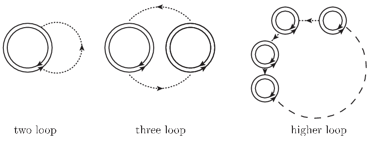
Higher loop terms are characterized by higher powers of the dimensionless quantity $\tilde{\lambda}/\triangle^{4}$ . However, as evident from (3.15), this quantity is order 1. Hence we must sum over all loops, which we describe below.

In each diagram in Figure 8, the two $Y^{I}$ s in a vertex $b_{ab}Y^{I}_{a}Y^{I}_{b}$ are contracted with two $Y^{J}$ s in a different vertex $b_{cd}Y^{J}_{c}Y^{J}_{d}$ . Therefore it is convenient to define a composite propagator²⁵²⁵ 25 See footnote 24 for another motivation for defining this propagator.

\displaystyle G_{(2)ab,cd}\equiv\sum_{I,J}\left(\langle Y^{I}_{a}Y^{J}_{c}\rangle\langle Y^{I}_{b}Y^{J}_{d}\rangle+\langle Y^{I}_{a}Y^{J}_{d}\rangle\langle Y^{I}_{b}Y^{J}_{c}\rangle\right)=\frac{2D}{\triangle^{4}}I_{ab,cd},

(B.5)

where $I_{ab,cd}$ is defined in (A.2) and it satisfies $M^{\prime}_{ab,cd}I_{cd,ef}=M^{\prime}_{ab,ef}$ . This composite propagator corresponds to one double line loop in Figure 7 and 8. By using this propagator, we can calculate the ( $n+1$ )-th loop correction to $N^{2}{\cal S}_{1}$ as

$\displaystyle-\frac{1}{(2n)!}\langle S_{int}^{2n}\rangle_{c}=$	$\displaystyle-\frac{1}{(2n)!}\left(\frac{-ig}{2}\right)^{2n}\langle b_{a_{1}b_{1}}Y_{a_{1}}^{I_{1}}Y_{b_{1}}^{I_{2}}\cdots b_{a_{2n}b_{2n}}Y_{a_{2n}}^{I_{2n}}Y_{b_{2n}}^{I_{2n}}\rangle_{c}$
$\displaystyle=$	$\displaystyle-\frac{(-)^{n}}{2n}\left(\frac{g^{2}D}{\triangle^{4}}\right)^{n}M^{\prime}_{a_{1}b_{1},a_{2}b_{2}}I_{a_{2}b_{2},a_{3}b_{3}}M^{\prime}_{a_{3}b_{3},a_{4}b_{4}}\cdots I_{a_{2n}b_{2n},a_{1}b_{1}}$
$\displaystyle=$	$\displaystyle-\frac{(-)^{n}}{2n}\left(\frac{g^{2}D}{\triangle^{4}}\right)^{n}{\rm Tr}M^{{}^{\prime}n}.$	(B.6)

Here $\langle\cdots\rangle_{c}$ denotes the connected diagram. ${\rm Tr}^{\prime}M^{n}$ has been calculated in (A.17). Now we can sum over $n$ and obtain the effective action,

$\displaystyle{\cal S}/D=$	$\displaystyle-\frac{N\triangle^{4}}{8\tilde{g}^{2}}+\frac{(N^{2}-1)}{4}\log\left(\frac{\triangle^{4}}{\tilde{g}^{2}N}\right)+\frac{N^{2}-1}{2D}\log\left(1+\frac{\tilde{g}^{2}N}{\triangle^{4}}\right)$
	$\displaystyle+\frac{N^{2}(N+1)(N-3)}{8D}\log\left(1+\frac{2\tilde{g}^{2}}{\triangle^{4}}\right)$
	$\displaystyle+\frac{N^{2}(N-1)(N+3)}{8D}\log\left(1-\frac{2\tilde{g}^{2}}{\triangle^{4}}\right)+O\left(\frac{1}{D^{2}}\right).$	(B.7)

Appendix C Evaluation of a toy integral using a complex saddle point

In Section 3, we evaluated the partition function (3.8) by a saddle point method. A similar calculation was done in Section 4. In this Appendix, we illustrate the procedure by considering a toy example.

Let us consider the integral

\displaystyle I=\int_{-\infty}^{\infty}dye^{-ay^{2}-by^{4}}~~~~~(a,b>0).

(C.1)

This integral can be evaluated by using the Bessel functions. Alternatively, if $b$ is small we can expand in powers of $b$ and obtain,

\displaystyle I=\sqrt{\frac{\pi}{a}}-\frac{3b\sqrt{\pi}}{4a^{5/2}}+\cdots.

(C.2)

Now we try to solve this integral by using the auxiliary variable. We can rewrite the integral as

		$\displaystyle\frac{1}{\sqrt{\pi b}}\int_{-\infty}^{\infty}dydx\exp\left(-ay^{2}-\frac{x^{2}}{b}+2ixy^{2}\right)$
	$\displaystyle=$	$\displaystyle\frac{1}{\sqrt{b}}\int_{-\infty}^{\infty}dx\exp\left(-\frac{x^{2}}{b}-\frac{1}{2}\log(a-2ix)\right).$		(C.3)

Let us try to evaluate this integral by using the saddle point method, in the limit $b\to 0$ . The exponent has two saddle points $x=-ia/4\pm i\sqrt{a^{2}+4b}/4$ . Since in the limit $b=0$ , the extremum is at $x=0$ , we should choose the saddle point corresponding to the “ $+$ ” sign. We get

\displaystyle I=\sqrt{\frac{\pi}{a}}-\frac{3b\sqrt{\pi}}{4a^{5/2}}+\cdots,

(C.4)

reproducing the earlier expression.

Appendix D The $Y$ -Propagator for $d=1$

In this section, we derive the $Y^{I}$ propagator in the $d=1$ model. The kinetic term of $Y^{I}$ in (2.15) can be written as,

		$\displaystyle\int_{0}^{\beta}dt{\rm Tr}\frac{1}{2}\left[Y^{I}\left(-D_{0}^{2}+\triangle^{2}\right)Y^{I}\right]$
		$\displaystyle=\frac{\beta}{2}\sum_{i,j,n}Y_{nij}^{I}\left(\frac{4\pi^{2}n^{2}}{\beta^{2}}-\frac{4\pi n(\alpha_{j}-\alpha_{i})}{\beta}+(\alpha_{j}-\alpha_{i})^{2}+\triangle^{2}\right)Y_{-nji}^{I},$		(D.1)

where we have used the constant diagonal gauge $A_{0ij}=\alpha_{i}\delta_{ij}$ and we have expanded $Y^{I}(t)=\sum_{n}Y_{n}^{I}e^{2\pi in/\beta}$ . We have also used the notation $B_{0}=i\triangle^{2}$ as in Section 4. Hence the propagator for each mode is given by

\displaystyle\langle Y_{nij}^{I}Y_{mkl}^{J}\rangle=\frac{1}{\beta}\frac{1}{\frac{4\pi^{2}n^{2}}{\beta^{2}}-\frac{4\pi n(\alpha_{j}-\alpha_{i})}{\beta}+(\alpha_{j}-\alpha_{i})^{2}+\triangle^{2}}\delta_{il}\delta_{jk}\delta^{IJ}\delta_{n+m,0}.

(D.2)

Then the propagator for $Y^{I}(t)$ becomes

$\displaystyle\langle Y_{ij}^{I}(t)Y_{kl}^{J}(0)\rangle$	$\displaystyle=\sum_{n}\frac{1}{\beta}\frac{e^{\frac{2\pi in}{\beta}t}}{\frac{4\pi^{2}n^{2}}{\beta^{2}}-\frac{4\pi n(\alpha_{j}-\alpha_{i})}{\beta}+(\alpha_{j}-\alpha_{i})^{2}+\triangle^{2}}\delta_{il}\delta_{jk}\delta^{IJ}$
	$\displaystyle=\sum_{n}\frac{-i}{4\pi\triangle}\Biggl[\frac{e^{\frac{2\pi in}{\beta}t}}{n-\frac{\beta(\alpha_{j}-\alpha_{i})}{2\pi}-i\frac{\beta\triangle}{2\pi}}-\frac{e^{\frac{2\pi in}{\beta}t}}{n-\frac{\beta(\alpha_{j}-\alpha_{i})}{2\pi}+i\frac{\beta\triangle}{2\pi}}\Biggr]\delta_{il}\delta_{jk}\delta^{IJ}$
	$\displaystyle=\frac{e^{i(\alpha_{j}-\alpha_{i})\|\|t\|\|}}{2\triangle}\Biggl[\frac{e^{-\triangle\|\|t\|\|}}{1-e^{i\beta(\alpha_{j}-\alpha_{i})}e^{-\beta\triangle}}-\frac{e^{\triangle\|\|t\|\|}}{1-e^{i\beta(\alpha_{j}-\alpha_{i})}e^{\beta\triangle}}\Biggr]\delta_{il}\delta_{jk}\delta^{IJ}.$	(D.3)

Here $||t||$ denotes $||t+n\beta||=t$ for $0\leq t<\beta$ . In order to derive it, we have used the formulae²⁶²⁶ 26 Eqns. (D.4), (E.25) and (E.33) are shown in [39].,

\displaystyle\sum_{n=-\infty}^{\infty}\frac{\sin(a-n)x}{a-n}=\pi,\quad\sum_{n=-\infty}^{\infty}\frac{\cos(a-n)x}{a-n}=\pi\cot(\pi a).

(D.4)

We can write the expression (D.3) further as

		$\displaystyle\langle Y_{ij}^{I}(t)Y_{kl}^{J}(0)\rangle=$
		$\displaystyle\frac{1}{2\triangle}\Biggl[e^{(i(\alpha_{j}-\alpha_{i})-\triangle)\|\|t\|\|}\sum_{n=0}^{\infty}x^{n}u^{j}_{n}u_{-n}^{i}+e^{(-i(\alpha_{j}-\alpha_{i})-\triangle)(\beta-\|\|t\|\|)}\sum_{n=0}^{\infty}x^{n}u^{j}_{-n}u_{n}^{i}\Biggr]\delta_{il}\delta_{jk}\delta^{IJ},$		(D.5)

where $x=e^{-\beta\triangle}$ and $u_{n}^{i}=e^{i\beta n\alpha_{i}}$ which satisfies $\sum_{i=1}^{N}u_{n}^{i}=Nu_{n}$ .

Appendix E All loop corrections up to $1/D$ in the $d=1$ model

In this appendix, we will show the derivation of the effective action of the $d=1$ model including the leading $1/D$ correction (4.21). This correction corresponds to ${\cal S}_{1,0}$ in (3.13) in the 0 dimensional model. Even in $d=1$ model (2.15), the same diagrams as in the $0$ dimensional model (Figure 8) will contribute. Therefore, as we discussed in Appendix B, the following composite propagator is convenient to calculate the loops,

\displaystyle\sum_{j,p,I,J}\langle Y_{ij}^{I}(t)Y_{pq}^{J}(t^{\prime})\rangle\langle Y_{jk}^{I}(t)Y_{lp}^{J}(t^{\prime})\rangle\equiv DN\sum_{n}G^{(2)}_{n,ik}e^{i\frac{2\pi n}{\beta}(t-t^{\prime})}\delta_{iq}\delta_{kl}.

(E.1)

Note that in this propagator we have only taken into account contractions which corresponds to planar diagrams. It turns out that the effective action obtained in this way corresponds to the leading term in a $1/N$ expansion. We will make a brief remark about non-planar terms at the end of this Appendix.

We can calculate this composite propagator by using (D.5) and a formula for Fourier integrals involving $||t||$ ,

\displaystyle\frac{1}{\beta^{2}}\int_{0}^{\beta}\int_{0}^{\beta}dtdt^{\prime}e^{s||t-t^{\prime}||}e^{-\frac{2\pi in}{\beta}t}e^{-\frac{2\pi im}{\beta}t^{\prime}}=\delta_{n+m,0}\frac{e^{s\beta}-1}{s\beta-2\pi in}.

(E.2)

Then the composite propagator can be obtained as

\displaystyle G^{(2)}_{n,ik}=\frac{1}{8\triangle^{2}}\left(P^{-}_{n,ik}S^{-}_{ik}+P^{+}_{n,ik}S^{+}_{ik}+Q_{n,ik}S_{Q,ik}\right),

(E.3)

where the $n$ -independent quantities are given by

$\displaystyle S^{-}_{ik}$	$\displaystyle=1+\sum_{m=1}^{\infty}x^{m}(u_{-m}^{i}u_{m}+u_{m}^{k}u_{-m}),$	(E.4)
$\displaystyle S^{+}_{ik}$	$\displaystyle=(S^{-}_{ik})^{*}=1+\sum_{m=1}^{\infty}x^{m}(u_{m}^{i}u_{-m}+u_{-m}^{k}u_{m}),$	(E.5)
$\displaystyle S_{Q,ik}$	$\displaystyle=x\sum_{l,m=0}^{\infty}x^{l+m}[u_{l+m+1}u_{-l}^{i}u_{-m}^{k}(u_{-1}^{i}-u_{-1}^{k})+u_{-(l+m+1)}u_{l}^{i}u_{m}^{k}(u_{1}^{k}-u_{1}^{i})],$	(E.6)

and the $n$ -dependent quantities are given by

	$\displaystyle P^{-}_{n,ik}$	$\displaystyle=\frac{1}{\pi i}\frac{-1}{\frac{i\beta(\alpha_{k}-\alpha_{i})-2\triangle\beta}{2\pi i}-n},\qquad P^{+}_{n,ik}=\frac{1}{\pi i}\frac{1}{\frac{i\beta(\alpha_{k}-\alpha_{i})+2\triangle\beta}{2\pi i}-n},$
	$\displaystyle Q_{n,ik}$	$\displaystyle=\frac{1}{\pi i}\frac{1}{\frac{i\beta(\alpha_{k}-\alpha_{i})}{2\pi i}-n}.$		(E.7)

By using the composite propagator (E.1), we can calculate the loop correction to the effective action as we studied in Appendix B. The $(n+1)$ -loop correction in Figure 8 is given by

\displaystyle-d_{n}\frac{(-)^{n}}{2n}\left(\beta g^{2}DN\right)^{n}\sum_{m=-\infty}^{\infty}\sum_{i,j=1}^{N}\left(G^{(2)}_{m,ij}\right)^{n},

(E.8)

where $d_{n}$ is a factor derived from the number of the planar diagrams and we can fix it by using (A.15),

\displaystyle d_{1}=-1,~~d_{2}=3,~~d_{n}=1~~(n\geq 3).

It is difficult to evaluate (E.8) in general. However, we are interested in the theory around the critical temperature $\bar{x}\sim 1/D$ where $\bar{x}$ is given by (4.9). Hence we can expand the effective potential with respect to $x$ and the lowest order of $x$ is enough to evaluate the $1/D$ correction. Especially, only the coefficient of $x|u_{1}|^{2}$ and $x^{2}|u_{1}|^{4}$ and the gauge-field independent terms will give us the relevant information of the dynamics around the critical points.

E.1 Two-loop correction

The two-loop correction to the effective action corresponds to the $n=1$ term in (E.8) and is given by

\displaystyle-\frac{1}{2}\beta g^{2}DN\sum_{i,j=1}^{N}\sum_{m=-\infty}^{\infty}G^{(2)}_{m,ij}.

(E.9)

We sum over the Fourier mode first.

	$\displaystyle\sum_{m=-\infty}^{\infty}P^{-}_{m,ij}$	$\displaystyle=1+2\sum_{m=1}^{\infty}x^{2m}u_{-m}^{i}u_{m}^{j},\quad\sum_{m=-\infty}^{\infty}P^{+}_{m,ij}=1+2\sum_{m=1}^{\infty}x^{2m}u_{m}^{i}u_{-m}^{j},$
	$\displaystyle\sum_{m=-\infty}^{\infty}Q_{m,ij}$	$\displaystyle=\frac{u_{-1}^{i}+u_{-1}^{j}}{u_{-1}^{i}-u_{-1}^{j}},$		(E.10)

where we have used (D.4). After summing over $i,j$ , we obtain the correction to the two-loop effective action as,

	$\displaystyle S^{two-loop}$	$\displaystyle=-\frac{N^{2}\beta\triangle}{8}\left(\frac{\tilde{\lambda}}{\triangle^{3}}\right)\left(1+2\sum_{m=1}^{\infty}(x^{2m}+2x^{m})\|u_{m}\|^{2}\right)+S_{int},$		(E.11)
	$\displaystyle S_{int}$	$\displaystyle=-\frac{N^{2}\beta\triangle}{4}\left(\frac{\tilde{\lambda}}{\triangle^{3}}\right)\left(x^{2}(u_{1}^{2}u_{-2}+u_{-1}^{2}u_{2})+O(x^{3})\right).$		(E.12)

Here we have omitted higher $x$ terms in the interaction, which are irrelevant around the critical points, as argued before.

We notice that this correction includes a cubic interaction $x^{2}u_{1}^{2}u_{-2}$ . Since the effective action (4.6) has the term $|u_{2}|^{2}/2$ arising from the gauge fixing, $|u_{1}|^{4}$ term can be induced through this interaction after integrating out $u_{2}$ . However, the coefficient of the $|u_{1}|^{4}$ terms obtained this way will be $O(x^{4})$ and we can ignore it compared to the $|u_{1}|^{4}$ potential in (4.26). Generally, we can show that the lowest order coefficient of the cubic interaction from the higher loops is also $x^{2}$ and we will ignore them here.

E.2 Three-loop correction

We evaluate the three-loop correction (the $n=2$ term in (E.8))

\displaystyle-\frac{3}{4}\left(\beta g^{2}DN\right)^{2}\sum_{m=-\infty}^{\infty}\sum_{i,j=1}^{N}\left(G^{(2)}_{m,ij}\right)^{2}.

(E.13)

In order to calculate the sum of the Fourier mode $m$ , we derive the product of $P^{\pm}$ and $Q$ as

	$\displaystyle P^{-}_{m,ij}P^{+}_{m,ij}$	$\displaystyle=\frac{1}{2\triangle\beta}\left(P^{-}_{m,ij}+P^{+}_{m,ij}\right),$
	$\displaystyle P^{-}_{m,ij}Q_{m,ij}$	$\displaystyle=\frac{1}{\triangle\beta}\left(P^{-}_{m,ij}+Q_{m,ij}\right),~~P^{+}_{m,ij}Q_{m,ij}=\frac{1}{\triangle\beta}\left(-P^{+}_{m,ij}+Q_{m,ij}\right).$		(E.14)

We also calculate the sum of squares of these quantities by using the formula

\displaystyle\sum_{m=-\infty}^{\infty}\left(\frac{1}{a-m}\right)^{2}=-\frac{\partial}{\partial a}\sum_{m=-\infty}^{\infty}\frac{1}{a-m}=\frac{\pi^{2}}{\sin^{2}\pi a}.

(E.15)

This leads to

	$\displaystyle\sum_{m=-\infty}^{\infty}(P^{-}_{m,ij})^{2}$	$\displaystyle=\frac{4x^{2}u_{-1}^{i}u_{1}^{j}}{(1-u_{-1}^{i}u_{1}^{j}x^{2})^{2}},\qquad\sum_{m=-\infty}^{\infty}\left(P^{+}_{m,ij}\right)^{2}=\frac{4x^{2}u_{1}^{i}u_{-1}^{j}}{(1-u_{1}^{i}u_{-1}^{j}x^{2})^{2}},$
	$\displaystyle\sum_{m=-\infty}^{\infty}\left(Q_{m,ij}\right)^{2}$	$\displaystyle=\frac{4u_{-1}^{i}u_{1}^{j}}{(1-u_{-1}^{i}u_{1}^{j})^{2}}.$		(E.16)

Now we can sum over $i,j$ and obtain the leading order of the corrections as

	$\displaystyle S^{three-loop}=$	$\displaystyle N^{2}\Biggl[-\frac{3}{128}\frac{\beta\tilde{\lambda}^{2}}{\triangle^{5}}+\left(-\frac{9}{32}\frac{\beta\tilde{\lambda}^{2}}{\triangle^{5}}x+O(x^{2})\right)\|u_{1}\|^{2}$
		$\displaystyle~~~+\left(-\frac{3}{32}\frac{\beta\tilde{\lambda}^{2}}{\triangle^{5}}x^{2}\left(\frac{5}{2}+\beta\triangle\right)+O(x^{3})\right)\|u_{1}\|^{4}\Biggr]+\cdots.$		(E.17)

E.3 $(n+1)$ -loop correction to effective potential

Up to three loops, the leading order of the coefficient of $|u_{1}|^{2}$ is $x$ and $|u_{1}|^{4}$ is $x^{2}$ in the $x$ expansion. We can find that these are true even in an arbitrary loop. Thus it is enough to fix the coefficient of these terms in each loop. In order to evaluate the $(n+1)$ -loop, we have to calculate

\displaystyle\sum_{m=-\infty}^{\infty}\sum_{i,j=1}^{N}\left(G^{(2)}_{m,ij}\right)^{n}=

\displaystyle\left(\frac{1}{8\triangle^{2}}\right)^{2}\sum_{m=-\infty}^{\infty}\sum_{i,j=1}^{N}\left(P^{-}_{m,ij}S^{-}_{ij}+P^{+}_{m,ij}S^{+}_{ij}+Q_{m,ij}S_{Q,ij}\right)^{n}.

(E.18)

in (E.8). However we can reduce this equation. Since $S_{Q,ij}$ is an order $x$ quantity as in (E.6), we can ignore $S_{Q}^{k}$ ( $k\geq 3$ ) terms here. Then we should evaluate only

	$\displaystyle\left(P^{-}S^{-}+P^{+}S^{+}\right)^{n}+nQS_{Q}\left(P^{-}S^{-}+P^{+}S^{+}\right)^{n-1}$
	$\displaystyle+\frac{n(n-1)}{2}\left(QS_{Q}\right)^{2}\left(P^{-}S^{-}+P^{+}S^{+}\right)^{n-2},$		(E.19)

where we have omitted the indices.

First we calculate the first term in (E.19). It is convenient to define $a_{k,l}=\left(P^{+}\right)^{k}\left(P^{-}\right)^{l}$ so that the equation becomes,

\displaystyle\left(P^{-}S^{-}+P^{+}S^{+}\right)^{n}

\displaystyle=\sum_{k=0}^{n}\binom{n}{k}a_{n-k,k}S_{+}^{n-k}S_{-}^{k}.

(E.20)

Through the relation (E.14), $a_{k,l}$ satisfy

\displaystyle a_{k,l}=\frac{1}{2\triangle\beta}\left(a_{k,l-1}+a_{k-1,l}\right).

(E.21)

Here we can approximate $a_{k,0}=a_{0,k}=0$ if $k\geq 2$ . This is because we can show that they are order $x^{2}$ quantities and the lowest order terms only contribute to $x^{2}|u_{1}|^{2}$ by using a similar logic as in (E.15) and (E.16). Then, through (E.21), we can obtain

	$\displaystyle a_{k,l}=$	$\displaystyle\frac{1}{(2\triangle\beta)^{k+l-1}}\sum_{k_{l-1}=1}^{k}\sum_{k_{l-2}=1}^{k_{l-1}}\cdots\sum_{k_{2}=1}^{k_{3}}\sum_{k_{1}=1}^{k_{2}}\left(a_{1,0}+a_{0,1}\right)$
	$\displaystyle=$	$\displaystyle\frac{1}{(2\triangle\beta)^{k+l-1}}\frac{(k+l-2)!}{(k-1)!(l-1)!}\left(a_{1,0}+a_{0,1}\right).$		(E.22)

Since $a_{1,0}=P^{+}_{m,ij}$ and $a_{0,1}=P^{-}_{m,ij}$ , we can sum over the $i,j$ and $m$ indices in (E.20) as

		$\displaystyle\sum_{m=-\infty}^{\infty}\sum_{i,j=1}^{N}\left(P^{+}_{m,ij}+P^{-}_{m,ij}\right)\left(S^{+}_{ij}\right)^{n-k}\left(S^{-}_{ij}\right)^{k}$
	$\displaystyle=$	$\displaystyle 2N^{2}\left(1+2nx\|u_{1}\|^{2}+n(n-1)x^{2}\|u_{1}\|^{4}+\cdots\right),$		(E.23)

where $\cdots$ denotes the irrelevant higher order terms. Then (E.20) becomes

\displaystyle\frac{2^{n}N^{2}}{(\triangle\beta)^{n-1}}\frac{(2n-3)!!}{(2n-2)!!}\left(1+2nx|u_{1}|^{2}+n(n-1)x^{2}|u_{1}|^{4}\right)+\cdots,

(E.24)

where we have used

\displaystyle\sum_{k=0}^{n}\binom{n}{k}\binom{n-2}{k-1}=2^{2(n-1)}\frac{(2n-3)!!}{(2n-2)!!}.

(E.25)

Next we evaluate

\displaystyle QS_{Q}\left(P^{-}S^{-}+P^{+}S^{+}\right)^{n-1},

(E.26)

in (E.19). First we can show that

\displaystyle\sum_{m=-\infty}^{\infty}\sum_{i,j=1}^{N}\left(P^{\pm}_{m,ij}\right)\left(S^{+}_{ij}\right)^{l}\left(S^{-}_{ij}\right)^{k}S_{Q,ij},

does not contribute to the relevant potential. Hence, by using (E.14), we obtain,

	$\displaystyle\sum_{m=-\infty}^{\infty}\sum_{i,j=1}^{N}Q_{m,ij}S_{Q,ij}\left(P_{m,ij}^{-}S^{-}_{ij}+P_{m,ij}^{+}S^{+}_{ij}\right)^{n-1}$
$\displaystyle=$	$\displaystyle\frac{1}{(\triangle\beta)^{n-1}}\sum_{m=-\infty}^{\infty}\sum_{i,j=1}^{N}Q_{m,ij}S_{Q,ij}\left(S^{-}_{ij}+S^{+}_{ij}\right)^{n-1}+\cdots$
$\displaystyle=$	$\displaystyle\frac{4N^{2}2^{n-1}}{(\triangle\beta)^{n-1}}\left(x\|u_{1}\|^{2}+(n-1)x^{2}\|u_{1}\|^{4}\right)+\cdots.$	(E.27)

Finally we evaluate

\displaystyle\left(QS_{Q}\right)^{2}\left(P^{-}S^{-}+P^{+}S^{+}\right)^{n-2}.

(E.28)

Here we can show that

\displaystyle\sum_{m=-\infty}^{\infty}\sum_{i,j=1}^{N}\left(P^{\pm}_{m,ij}\right)\left(S^{+}_{ij}\right)^{k}\left(S^{-}_{ij}\right)^{l}S_{Q,ij}^{2},

does not contribute to the relevant potential. Thus we obtain

		$\displaystyle\sum_{m=-\infty}^{\infty}\sum_{i,j=1}^{N}\left(Q_{m,ij}S_{Q,ij}\right)^{2}\left(P_{m,ij}^{-}S^{-}_{ij}+P_{m,ij}^{+}S^{+}_{ij}\right)^{n-2}$
	$\displaystyle=$	$\displaystyle\frac{2^{n-2}}{(\triangle\beta)^{n-2}}\sum_{m=-\infty}^{\infty}\sum_{i,j=1}^{N}\left(Q_{m,ij}S_{Q,ij}\right)^{2}+\cdots=\frac{2^{n-2}}{(\triangle\beta)^{n-2}}\left(8N^{2}x^{2}\|u_{1}\|^{4}\right)+\cdots.$		(E.29)

Let us summarize all relevant terms of the $(n+1)$ -loop effective action. The gauge-field independent term becomes

\displaystyle-(-)^{n}d_{n}N^{2}\beta\triangle\left(\frac{\tilde{\lambda}}{4\triangle^{3}}\right)^{n}\frac{(2n-3)!!}{(2n)!!}.

(E.30)

Note that this result is exact. The leading $|u_{1}|^{2}$ potential in the $x$ expansion is given by

\displaystyle-(-)^{n}d_{n}N^{2}\beta\triangle\left(\frac{\tilde{\lambda}}{4\triangle^{3}}\right)^{n}\left(\frac{(2n-3)!!}{(2n-2)!!}+1\right)x|u_{1}|^{2}+O(x^{2}).

(E.31)

The leading $|u_{1}|^{4}$ potential is

\displaystyle-(-)^{n}d_{n}N^{2}\beta\triangle\frac{n-1}{2}\left(\frac{\tilde{\lambda}}{4\triangle^{3}}\right)^{n}\left(\frac{(2n-3)!!}{(2n-2)!!}+2+\triangle\beta\right)x^{2}|u_{1}|^{4}+O(x^{3}).

(E.32)

We can sum over $n$ by using the following formula:

\displaystyle\sum_{n=1}^{\infty}(-)^{n-1}\frac{(2n-3)!!}{(2n)!!}x^{n}=\sqrt{1+x}-1,

(E.33)

and its derivative with respect to $x$ . With this, we finally obtain the effective action (4.21).

Note that it is possible to extend the calculation in this section to finite $N$ case as we have done in the $d=0$ model. The finite $N$ result for the gauge-field independent constant term is simply obtained by replacing $d_{n}N^{n+2}$ in (E.30) with ${\rm Tr}M^{{}^{\prime}n}$ in (A.17). The terms including the gauge potential are more complicated and we have to modify the composite propagator (E.1).

References

[1] E. Brezin and S. R. Wadia, “The Large N expansion in quantum field theory and statistical physics: From spin systems to two-dimensional gravity,” Singapore, Singapore: World Scientific (1993) 1130 p
[2] T. Eguchi and H. Kawai, “Reduction Of Dynamical Degrees Of Freedom In The Large N Gauge Theory,” Phys. Rev. Lett. 48, 1063 (1982).
[3] W. Krauth and M. Staudacher, “Eigenvalue distributions in Yang-Mills integrals,” Phys. Lett. B 453, 253 (1999) [arXiv:hep-th/9902113].
[4] T. Banks, W. Fischler, S. H. Shenker and L. Susskind, “M theory as a matrix model: A conjecture,” Phys. Rev. D 55, 5112 (1997) [arXiv:hep-th/9610043].
[5] N. Ishibashi, H. Kawai, Y. Kitazawa and A. Tsuchiya, “A large-N reduced model as superstring,” Nucl. Phys. B 498, 467 (1997) [arXiv:hep-th/9612115].
[6] T. Hotta, J. Nishimura and A. Tsuchiya, “Dynamical aspects of large N reduced models,” Nucl. Phys. B 545, 543 (1999) [arXiv:hep-th/9811220].
[7] N. Itzhaki, J. M. Maldacena, J. Sonnenschein and S. Yankielowicz, “Supergravity and the large N limit of theories with sixteen supercharges,” Phys. Rev. D 58, 046004 (1998) [arXiv:hep-th/9802042].
[8] D. N. Kabat, G. Lifschytz and D. A. Lowe, “Black hole thermodynamics from calculations in strongly coupled gauge theory,” Int. J. Mod. Phys. A 16, 856 (2001) [Phys. Rev. Lett. 86, 1426 (2001)] [arXiv:hep-th/0007051].
[9] D. N. Kabat, G. Lifschytz and D. A. Lowe, “Black hole entropy from non-perturbative gauge theory,” Phys. Rev. D 64, 124015 (2001) [arXiv:hep-th/0105171].
[10] K. N. Anagnostopoulos, M. Hanada, J. Nishimura and S. Takeuchi, “Monte Carlo studies of supersymmetric matrix quantum mechanics with sixteen supercharges at finite temperature,” Phys. Rev. Lett. 100, 021601 (2008) [arXiv:0707.4454 [hep-th]].
[11] M. Hanada, A. Miwa, J. Nishimura and S. Takeuchi, “Schwarzschild radius from Monte Carlo calculation of the Wilson loop in supersymmetric matrix quantum mechanics,” Phys. Rev. Lett. 102 (2009) 181602 [arXiv:0811.2081 [hep-th]].
[12] M. Hanada, Y. Hyakutake, J. Nishimura and S. Takeuchi, “Higher derivative corrections to black hole thermodynamics from supersymmetric matrix quantum mechanics,” Phys. Rev. Lett. 102 (2009) 191602 [arXiv:0811.3102 [hep-th]].
[13] S. Catterall and T. Wiseman, “Black hole thermodynamics from simulations of lattice Yang-Mills theory,” Phys. Rev. D 78, 041502 (2008) [arXiv:0803.4273 [hep-th]].
[14] T. Azeyanagi, M. Hanada, H. Kawai and Y. Matsuo, “Worldsheet Analysis of Gauge/Gravity Dualities,” Nucl. Phys. B 816, 278 (2009) [arXiv:0812.1453 [hep-th]].
[15] B. Sundborg, “The Hagedorn Transition, Deconfinement and N=4 SYM Theory,” Nucl. Phys. B 573, 349 (2000) [arXiv:hep-th/9908001].
[16] O. Aharony, J. Marsano, S. Minwalla, K. Papadodimas and M. Van Raamsdonk, “The Hagedorn / deconfinement phase transition in weakly coupled large N gauge theories,” Adv. Theor. Math. Phys. 8, 603 (2004) [arXiv:hep-th/0310285].
[17] L. Alvarez-Gaume, C. Gomez, H. Liu and S. Wadia, “Finite temperature effective action, AdS(5) black holes, and 1/N expansion,” Phys. Rev. D 71, 124023 (2005) [arXiv:hep-th/0502227].
[18] L. Alvarez-Gaume, P. Basu, M. Marino and S. R. Wadia, “Blackhole / string transition for the small Schwarzschild blackhole of AdS(5) x S**5 and critical unitary matrix models,” Eur. Phys. J. C 48, 647 (2006) [arXiv:hep-th/0605041].
[19] D. E. Berenstein, J. M. Maldacena and H. S. Nastase, “Strings in flat space and pp waves from N = 4 super Yang Mills,” JHEP 0204, 013 (2002) [arXiv:hep-th/0202021].
[20] I. R. Klebanov, J. M. Maldacena and N. Seiberg, “D-brane decay in two-dimensional string theory,” JHEP 0307, 045 (2003) [arXiv:hep-th/0305159].
[21] J. McGreevy and H. L. Verlinde, “Strings from tachyons: The c = 1 matrix reloaded,” JHEP 0312, 054 (2003) [arXiv:hep-th/0304224].
[22] O. Aharony, J. Marsano, S. Minwalla and T. Wiseman, “Black hole-black string phase transitions in thermal 1+1-dimensional supersymmetric Yang-Mills theory on a circle,” Class. Quant. Grav. 21, 5169 (2004) [arXiv:hep-th/0406210].
[23] O. Aharony, J. Marsano, S. Minwalla, K. Papadodimas, M. Van Raamsdonk and T. Wiseman, “The phase structure of low dimensional large N gauge theories on tori,” JHEP 0601, 140 (2006) [arXiv:hep-th/0508077].
[24] N. Kawahara, J. Nishimura and S. Takeuchi, “Phase structure of matrix quantum mechanics at finite temperature,” JHEP 0710, 097 (2007) [arXiv:0706.3517 [hep-th]].
[25] T. Azeyanagi, M. Hanada, T. Hirata and H. Shimada, JHEP 0903 (2009) 121 [arXiv:0901.4073 [hep-th]].
[26] D. J. Gross and E. Witten, “Possible Third Order Phase Transition In The Large N Lattice Gauge Theory,” Phys. Rev. D 21, 446 (1980).
[27] S. R. Wadia, “N = Infinity Phase Transition In A Class Of Exactly Soluble Model Lattice Gauge Theories,” Phys. Lett. B 93, 403 (1980).
[28] S. Wadia, “A Study Of U(N) Lattice Gauge Theory In Two-Dimensions,” preprint EFI-79/44-CHICAGO.
[29] J. M. Drouffe and J. B. Zuber, Phys. Rept. 102 (1983) 1.
[30] G. Mandal, M. Mahato, T. Morita and S. R. Wadia, in progress.
[31] A. Jevicki and B. Sakita, “The quantum collective field method and its application to the planar limit,” Nucl. Phys. B 165, 511 (1980).
[32] J. Jurkiewicz and K. Zalewski, “Vacuum Structure Of The U(N $\to$ Infinity) Gauge Theory On A Two-Dimensional Lattice For A Broad Class Of Variant Actions,” Nucl. Phys. B 220, 167 (1983).
[33] G. Mandal, “Phase structure of unitary matrix models,” Mod. Phys. Lett. A 5, 1147 (1990).
[34] R. Gregory and R. Laflamme, “Black strings and p-branes are unstable,” Phys. Rev. Lett. 70, 2837 (1993) [arXiv:hep-th/9301052].
[35] B. Kol, “The Phase Transition between Caged Black Holes and Black Strings - A Review,” Phys. Rept. 422, 119 (2006) [arXiv:hep-th/0411240].
[36] W. Taylor, “D-brane field theory on compact spaces,” Phys. Lett. B 394, 283 (1997) [arXiv:hep-th/9611042].
[37] L. Susskind, “Matrix theory black holes and the Gross Witten transition,” arXiv:hep-th/9805115.
[38] R. Slansky, “Group Theory For Unified Model Building,” Phys. Rept. 79, 1 (1981).
[39] S. Moriguchi, K. Udagawa and S. Hitotsumatsu, “Sugaku Koushiki II,” Iwanami, Tokyo (in Japanese), (2001) 340 p

1 Introduction and Summary

2 The d=1d=1 model: preliminaries

3 The d=0d=0 model

3.1 The large DD limit

3.2 Large D,ND,N limit

3.3 The saddle point

4 The d=1d=1 model: result

4.1 Computation of 𝒮⁡(△,{un}){\cal S}(\triangle,\{u_{n}\}) in leading large DD

High temperature:

(a) Small |u1||u_{1}| approximation:

(b) Large DD limit vs 1/D1/D expansion:

4.2 1/D1/D correction to the effective action

4.3 1/D1/D expansion vs. numerical calculation

1/D1/D expansion for small DD:

5 D brane interpretation

6 Conclusion

Acknowledgement

Appendix A Some results involving Ma​b,c​dM_{ab,cd}

A.1 Algebraic properties of Ma​b,c​dM_{ab,cd}

A.2 Results involving Ma​b,c​dM_{ab,cd}

The inverse M−1M^{-1}:

Eigenvalue of Ma​b,c​dM_{ab,cd}:

Calculation of Tr​Mn{\rm Tr}M^{n}:

Appendix B Details of the d=0d=0 model

B.1 Calculation of 𝒮1{\cal S}_{1}: the 1/D1/D correction

Appendix C Evaluation of a toy integral using a complex saddle point

Appendix D The YY-Propagator for d=1d=1

Appendix E All loop corrections up to 1/D1/D in the d=1d=1 model

E.1 Two-loop correction

E.2 Three-loop correction

E.3 (n+1)(n+1)-loop correction to effective potential

References

2 The $d=1$ model: preliminaries

3 The $d=0$ model

3.1 The large $D$ limit

3.2 Large $D,N$ limit

4 The $d=1$ model: result

4.1 Computation of ${\cal S}(\triangle,\{u_{n}\})$ in leading large $D$

(a) Small $|u_{1}|$ approximation:

(b) Large $D$ limit vs $1/D$ expansion:

4.2 $1/D$ correction to the effective action

4.3 $1/D$ expansion vs. numerical calculation

$1/D$ expansion for small $D$ :

Appendix A Some results involving $M_{ab,cd}$

A.1 Algebraic properties of $M_{ab,cd}$

A.2 Results involving $M_{ab,cd}$

The inverse $M^{-1}$ :

Eigenvalue of $M_{ab,cd}$ :

Calculation of ${\rm Tr}M^{n}$ :

Appendix B Details of the $d=0$ model

B.1 Calculation of ${\cal S}_{1}$ : the $1/D$ correction

Appendix D The $Y$ -Propagator for $d=1$

Appendix E All loop corrections up to $1/D$ in the $d=1$ model

E.3 $(n+1)$ -loop correction to effective potential